Quantum Monte Carlo simulation of a two-dimensional Bose gas

Abstract

The equation of state of a homogeneous two-dimensional Bose gas is calculated using quantum Monte Carlo methods. The low-density universal behavior is investigated using different interatomic model potentials, both finite-ranged and strictly repulsive and zero-ranged supporting a bound state. The condensate fraction and the pair distribution function are calculated as a function of the gas parameter, ranging from the dilute to the strongly correlated regime. In the case of the zero-range pseudopotential we discuss the stability of the gas-like state for large values of the two-dimensional scattering length, and we calculate the critical density where the system becomes unstable against cluster formation.

I Introduction

Degenerate low-dimensional gases are presently attracting considerable interest as model systems to investigate beyond mean-field effects and phenomena where many-body correlations, thermal and quantum fluctuations play a relevant role LesHouches . In two dimensions (2D), it is well known that thermal excitations destroy long-range order and Bose-Einstein condensation (BEC) can not exist in large bosonic systems at finite temperature Hohenberg . Nevertheless, a defect-mediated phase transition from a high-temperature normal fluid to a low-temperature superfluid was predicted by Berezinskii, Kosterlitz and Thouless (BKT) BKT and has been observed in thin films of liquid ⁴He Reppy . At zero temperature, fluctuations are instead negligible and BEC is possible. The ground-state energy per particle of a homogeneous dilute Bose gas in 2D has been first calculated by Schick Schick and is given by

$$\frac{E_{MF}}{N}=\frac{2\pi\hbar^{2}}{m}\frac{n}{\log(1/na_{2D}^{2})}\;,$$ (1)

where $m$ is the mass of the particles, $n$ is the number density and $a_{2D}$ is the 2D scattering length. The above result holds for small values of the gas parameter, $na_{2D}^{2}\ll 1$, and can be obtained within a mean-field approximation using the coupling constant

$$g_{2D}=\frac{4\pi\hbar^{2}}{m}\frac{1}{\log(1/na_{2D}^{2})}\;.$$ (2)

The presence at low energy of a density dependent coupling constant is a peculiar feature of 2D systems.

Bose gases in quasi-2D have been realized with spin-polarized hydrogen on a liquid-helium surface Safonov and with alkali-metal atoms confined in highly anisotropic harmonic traps EXP ; Grimm ; Foot . In these systems, the transverse motion of the atoms is frozen to zero-point oscillations resulting in fully 2D kinematics, but the interatomic scattering processes are still three-dimensional (3D). In fact, the 3D s-wave scattering length $a_{3D}$ is always much smaller than the characteristic length of the tight transverse confinement. Theoretical studies of quasi-2D trapped systems predict the existence of a low-temperature quasicondensate phase Popov ; Petrov1 whose properties have been investigated using mean-field approaches MF . The nature of the transition in confined systems and whether it belongs to the BEC or BKT universality class is still an open problem both experimentally and theoretically.

An important theoretical prediction for quasi-2D Bose gases in harmonic traps is the renormalization of the coupling constant due to the tight confinement in one direction. To logarithmic accuracy the result is given by Petrov1 ; Petrov2

$$g_{2D}=\frac{2\sqrt{2\pi}\hbar^{2}}{m}\frac{1}{\frac{a_{z}}{a_{3D}}+\frac{1}{\sqrt{2\pi}}\log(1/n(0)a_{z}^{2})}\;,$$ (3)

where $a_{z}=\sqrt{\hbar/m\omega_{z}}$ is the harmonic oscillator length, fixed by the frequency $\omega_{z}$ of the tight transverse confinement, and $n(0)$ is the 2D density in the center of the trap. If $a_{3D}\ll a_{z}$, one can neglect the $\log$ term in Eq. (3) and the resulting coupling constant is determined by the 3D scattering length. On the contrary, if $a_{3D}\gg a_{z}$, $g_{2D}$ becomes independent of the value of $a_{3D}$ and a regime of pure 2D scattering is achieved with $a_{2D}=a_{z}$. This universal regime, where the properties of the system only depend on density and not on interaction, is highly interesting and can be realized in trapped gases by using a Feshbach resonance Feshbach to achieve large values for $a_{3D}$.

In this work we investigate the ground-state properties of a strictly 2D homogeneous Bose gas using quantum Monte Carlo techniques. We determine the equation of state over a wide range of values of the gas parameter from the extremely dilute regime, $na_{2D}^{2}\sim 10^{-7}$, to the strongly correlated regime, $na_{2D}^{2}\sim 0.1$. The calculations of the energy per particle are carried out using three different interatomic model potentials: two repulsive finite-ranged potentials and a zero-range pseudopotential which supports a two-body bound state. We investigate beyond mean-field corrections to the equation of state (1) and their dependence on the gas parameter $na_{2D}^{2}$. In the case of the zero-range pseudopotential, from a study of the system compressibility as a function of the gas parameter we estimate that $na_{2D}^{2}\simeq 0.04$ is the critical density at which the gas-like state becomes unstable against cluster formation. This result puts an upper limit to the value of density that can be reached in harmonic traps when one enters the regime of pure 2D scattering. We also report results of the pair distribution function and the condensate fraction as a function of the gas parameter.

The structure of the paper is as follows. In Section II we introduce the many-body Hamiltonian and the model interatomic potentials we use in the simulations. We also discuss the quantum Monte Carlo methods employed in the present study and the choice of the trial wave functions. Section III containes the results obtained and Section IV draws our conclusions.

II Method

We consider a homogeneous system of $N$ spinless bosons in 2D described by the many-body Hamiltonian

$$H=-\frac{\hbar^{2}}{2m}\sum_{i=1}^{N}\nabla_{i}^{2}+\sum_{i<j}V({\bf r}_{i}-{\bf r}_{j})\;,$$ (4)

where ${\bf r}_{i}=x_{i}\hat{\bf i}+y_{i}\hat{\bf j}$ denotes the 2D position vector of the $i$-th particle and $V({\bf r})$ is the two-body interatomic potential. We use different choices for the interatomic potential $V({\bf r})$:

(i) Hard-disk (HD) potential defined by

$$V^{HD}({\bf r})=\left\{\begin{array}[]{cll}\infty&(r<a_{2D})\\ 0&(r>a_{2D})\;,\end{array}\right.$$ (7)

in which case the hard-disk diameter corresponds to the scattering length $a_{2D}$.

(ii) Soft-disk (SD) potential defined by

$$V^{SD}({\bf r})=\left\{\begin{array}[]{cll}V_{0}&(r<R)\\ 0&(r>R)\;,\end{array}\right.$$ (10)

in which case the scattering length is given in terms of the modified Bessel function $I_{0}(x)$ and its derivative $I_{0}^{\prime}(x)$,

$$a_{2D}=R\exp\left[-\frac{1}{RK_{0}}\frac{I_{0}(RK_{0})}{I_{0}^{\prime}(RK_{0})}\right]\;,$$ (11)

where $K_{0}^{2}=mV_{0}/\hbar^{2}$ with $V_{0}>0$. For a finite $V_{0}$ one has always $R>a_{2D}$; if $V_{0}\to+\infty$ the SD and HD potentials coincide with $a_{2D}=R$. In the present calculations, the range of the SD potential is kept fixed to the value $R=5a_{2D}$ and the height $V_{0}$ is determined through Eq. (11) to give the desired value of $a_{2D}$.

(iii) Zero-range pseudopotential (PP) defined by OLP

$$V^{PP}({\bf r})=-\frac{2\pi\hbar^{2}}{m}\frac{\delta({\bf r})}{\log(qa_{2D})}\left[1-\log(qr)r\frac{\partial}{\partial r}\right]\;,$$ (12)

where the second term in the square brackets is a regularizing operator with $q$ an arbitrary wave vector. The potential $V^{PP}(r)$ supports a two-body bound state with energy $\epsilon_{b}=-4\hbar^{2}/(ma_{2D}^{2}e^{2\gamma})$ and wave function $f_{b}(r)=K_{0}(2r/(a_{2D}e^{\gamma}))$, where $K_{0}(x)$ is the modified Bessel function and $\gamma\simeq 0.577$ is the Euler constant.

The calculations with the repulsive potentials $V^{HD}(r)$ and $V^{SD}(r)$ are carried out using the diffusion Monte Carlo (DMC) method. This technique solves the many-body time-independent Schrödinger equation by evolving the function $f({\bf R},\tau)=\psi_{T}({\bf R})\Psi({\bf R},\tau)$ in imaginary time $\tau=it/\hbar$ according to the time-dependent Schrödinger equation

$$-\frac{\partial f({\bf R},\tau)}{\partial\tau}= - D\nabla_{\bf R}^{2}f({\bf R},\tau)+D\nabla_{\bf R}[{\bf F}({\bf R})f({\bf R},\tau)]$$ (13)

$$+ [E_{L}({\bf R})-E_{ref}]f({\bf R},\tau)\;.$$

Here $\Psi({\bf R},\tau)$ denotes the wave function of the system and $\psi_{T}({\bf R})$ is a trial function used for importance sampling. In the above equation ${\bf R}=({\bf r}_{1},...,{\bf r}_{N})$, $E_{L}({\bf R})=\psi_{T}({\bf R})^{-1}H\psi_{T}({\bf R})$ denotes the local energy, ${\bf F}({\bf R})=2\psi_{T}({\bf R})^{-1}\nabla_{\bf R}\psi_{T}({\bf R})$ is the quantum drift force, $D=\hbar^{2}/(2m)$ plays the role of an effective diffusion constant, and $E_{ref}$ is a reference energy introduced to stabilize the numerics. The energy and other observables of the ground state of the system are calculated from averages over the asymptotic distribution function $f({\bf R},\tau\to\infty)$. Apart from statistical errors, the DMC method determines the ground-state energy of a system of $N$ bosons exactly.

In the case of the pseudopotential $V^{PP}(r)$, Eq. (12), the gas-like state is not the ground state of the system, but is a highly-excited state of the Hamiltonian. We expect, however, that for small values of the gas parameter, $na_{2D}^{2}\ll 1$, the gas-like state is stable against formation of many-body bound states. The calculations with the PP potential are performed at the level of the variational Monte Carlo (VMC) method to avoid the technical difficulties that arise in the study of excited states in the DMC method. Nevertheless, as it will be shown in Section III, the accuracy achieved by using this variational approach is very high. The VMC technique is based on the variational principle

$$\frac{\langle\psi_{T}|H|\psi_{T}\rangle}{\langle\psi_{T}|\psi_{T}\rangle}\geq E\;,$$ (14)

which is here applied to excited states of the Hamiltonian $H$. For a trial wave function $\psi_{T}$ with a given symmetry, the variational estimate provides an upper bound to the energy $E$ of the lowest excited state of the Hamiltonian $H$ with that symmetry.

In all the calculations the trial wave function $\psi_{T}({\bf R})$ is taken of the Jastrow form

$$\psi_{T}({\bf r}_{1},...,{\bf r}_{N})=\prod_{i<j}f(r_{ij})\;,$$ (15)

where the correlation factor $f(r)$ is chosen as the solution of the two-body Schrödinger equation subject to the boundary conditions $f(r\geq d)=1$ and $f^{\prime}(r\geq d)=0$ on the wave function and its first derivative respectively, with $d$ a variational parameter. For the repulsive potentials, HD and SD, $f(r)$ corresponds to the ground-state two-body wave function. On the contrary, in the case of the PP interaction, $f(r)$ is chosen as the two-body wave function corresponding to the lowest excited state with positive energy. The pseudopotential $V^{PP}$ imposes the following boundary condition on the pair wave function for zero interparticle distance

$$\frac{\left[rf^{\prime}(r)\right]_{r=0}}{\left[f(r)-\log(qr)rf^{\prime}(r)\right]_{r=0}}=-\frac{1}{\log(qa_{2D})}\;.$$ (16)

The free two-particle problem in 2D $-\hbar^{2}/m\nabla^{2}f(r)=\hbar^{2}k^{2}/mf(r)$, holding for $r\neq 0$, gives the general solution

$$f(r)=AJ_{0}(kr)+BY_{0}(kr)\;,$$ (17)

in terms of the $J_{0}(x)$ and $Y_{0}(x)$ Bessel functions. The boundary condition (16) is imposed by the relation

$$a_{2D}=\frac{2e^{-\gamma}}{k}\exp\left(-\frac{\pi A}{2B}\right)\;.$$ (18)

In addition we require that $f(r)$ possess only one node for distances $0<r<d$. The boundary conditions at $r=d$ together with (18) fix the values of the constants $A$ and $B$ and of the wavevector $k$. If $d\gg a_{2D}$, the eigenenergy $\hbar^{2}k^{2}/m$ is small and the node of $f(r)$ is located at $r=a_{2D}$.

All the Monte Carlo calculations have been carried out considering periodic boundary conditions with a cubic simulation box whose size $L$ is fixed by the density $n$ and by the total number of atoms: $n=N/L^{2}$. The healing length $d$ is considered everywhere $d=L/2$ since a VMC optimization has shown that this is a good option.

Table 1: Energy per particle $E/N$ corresponding to the model potentials $V^{HD}(r)$ (DMC results), $V^{SD}(r)$ (DMC results) and $V^{PP}(r)$ (VMC results) [energies are in units of $\hbar^{2}/(2ma_{2D}^{2})$].

$na_{2D}^{2}$	$HD$	$SD$	$PP$
$1\times 10^{-7}$	$7.738(3)\times 10^{-8}$	$7.732(6)\times 10^{-8}$
$3\times 10^{-7}$	$2.500(1)\times 10^{-7}$	$2.498(1)\times 10^{-7}$
$1\times 10^{-6}$	$9.103(5)\times 10^{-7}$	$0.909(1)\times 10^{-6}$	$9.162(7)\times 10^{-7}$
$3\times 10^{-6}$	$2.982(2)\times 10^{-6}$	$2.977(4)\times 10^{-6}$
$1\times 10^{-5}$	$1.108(2)\times 10^{-5}$	$1.106(1)\times 10^{-5}$	$1.115(1)\times 10^{-5}$
$3\times 10^{-5}$	$3.710(4)\times 10^{-5}$	$3.702(2)\times 10^{-5}$
$1\times 10^{-4}$	$1.417(1)\times 10^{-4}$	$1.415(1)\times 10^{-4}$	$1.428(1)\times 10^{-4}$
$3\times 10^{-4}$	$4.922(5)\times 10^{-4}$	$4.910(2)\times 10^{-4}$
$1\times 10^{-3}$	$1.981(4)\times 10^{-3}$	$1.972(1)\times 10^{-3}$	$1.994(1)\times 10^{-3}$
$3\times 10^{-3}$	$7.34(2)\times 10^{-3}$	$7.224(3)\times 10^{-3}$
$1\times 10^{-2}$	$3.296(5)\times 10^{-2}$	$3.057(2)\times 10^{-2}$	$3.304(4)\times 10^{-2}$
$3\times 10^{-2}$	$1.436(2)\times 10^{-1}$	$1.105(1)\times 10^{-1}$	$1.369(6)\times 10^{-1}$
$1\times 10^{-1}$	$8.94(2)\times 10^{-1}$	$4.161(4)\times 10^{-1}$

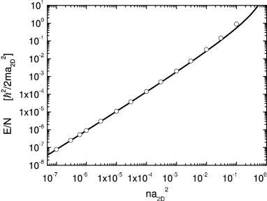
Figure 1: Energy per particle as a function of the gas parameter for the HD potential. Solid line: mean-field result, Eq. (1). Error bars are smaller than the size of the symbols.

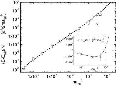
Figure 2: Beyond mean-field corrections to the equation of state. Circles, HD potential; triangles: SD potential; squares: PP potential. Dashed line: numerical fit to the results of the HD potential, Eq. (III). Error bars are smaller than the size of the symbols. Inset: region of extremely dilute systems $na_{2D}^{2}\leq 10^{-6}$.

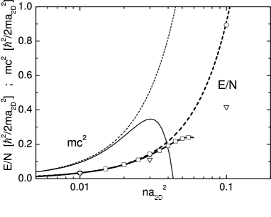
Figure 3: Energy per particle and inverse compressibility as a function of the gas parameter. Symbols are as in Fig. 2. Thick and thin dashed lines: best fit (III) to the HD equation of state and corresponding $mc^{2}$, respectively. Thick and thin solid line: polynomial best fit to the PP equation of state and corresponding $mc^{2}$, respectively. Error bars are smaller than the size of the symbols.

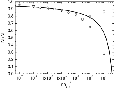
Figure 4: Condensate fraction as a function of the gas parameter. Circles, HD potential; triangles, SD potential. Solid line: result from Bogoliubov theory, Eq. (21).

Figure 5: Pair distribution function of a HD gas obtained for three values of the gas parameter: $na_{2D}^{2}=10^{-4}$, solid line; $na_{2D}^{2}=0.01$, dashed line; $na_{2D}^{2}=0.1$, dotted line.

III Results

The numerical simulations are carried out with $N=512$ particles for the lowest densities ($na_{2D}^{2}\leq 10^{-4}$) and with $N=256$ particles for the rest. The DMC results for the energy per particle corresponding to the HD potential are reported in Table LABEL:tab1 as a function of the gas parameter. Variational results on the same system have been obtained in the dilute regime by Mazzanti et al. Mazzanti using Correlated Basis Functions theory and at high densities by Lei Xing MCARLO1 and Solís MCARLO2 using VMC. In Fig. 1, the DMC results for the HD system are compared with the mean-field result, Eq. (1). We find a remarkably good agreement up to large values of $na_{2D}^{2}$. It is worth noticing that the range of validity of the mean-field approximation is in 2D significantly larger than the one observed in 3D US . Beyond mean-field corrections to the equation of state are shown in Fig. 2, where we plot the difference $(E-E_{MF})/N$ for the three model potentials: $V^{HD}(r)$ (DMC results), $V^{SD}(r)$ (DMC results) and $V^{PP}(r)$ (VMC results). Focusing on the exact DMC results, one can notice the universal behavior of the equation of state for $na_{2D}^{2}\ll 1$. The results of the HD and SD model potentials are practically indistinguishable up to $na_{2D}^{2}\sim 10^{-2}$ (see Table LABEL:tab1), showing that beyond mean-field corrections to Eq. (1) only depend on the value of the gas parameter $na_{2D}^{2}$ and not on the details of the interatomic potential. By increasing $na_{2D}^{2}$ the results obtained with the SD potential (triangles in Fig. 2) start to deviate from the ones corresponding to the HD potential (circles in Fig. 2) approximately about $na_{2D}^{2}\sim 0.01$. The VMC results for the PP potential are upper bounds to the eigenenergy of the gas-like state. However, looking at Table LABEL:tab1 and Fig. 2, one can see that they are nearly indistinguishable from the exact HD and SD energies in the low-density regime. A similar accuracy for the energy of the gas-like state is expected also for larger values of the gas parameter, where the results of the PP interaction start to separate from the HD ones as the effects of the finite interaction range become more important. It is also worth noticing that for the smallest values of $na_{2D}^{2}$ (inset of Fig. 2) the beyond mean-field correction is negative. This is consistent with the perturbation expansion PEXP

$$\frac{E-E_{MF}}{N}=-\frac{2\pi\hbar^{2}n}{m}\frac{\log[\log(1/na_{2D}^{2})]}{[\log(na_{2D}^{2})]^{2}}\;,$$ (19)

which is expected to hold if $\log[\log(1/na_{2D}^{2})]\gg 1$. For our smallest value of the gas parameter, $na_{2D}^{2}=10^{-7}$, one finds $\log[\log(1/na_{2D}^{2})]\simeq 2.8$. We fit the HD equation of state using the expression

$$\frac{E-E_{MF}}{N} = \frac{2\pi\hbar^{2}n}{m}$$

$$\times \left[-A\frac{\log[\log(1/na_{2D}^{2})]}{[\log(na_{2D}^{2})]^{2}}+\frac{B}{[\log(na_{2D}^{2})]^{2}}\right]\;,$$

where $A$ and $B$ are free parameters. The best fit to all HD points, with the exclusion of the one at the highest density $na_{2D}^{2}=0.1$, gives $A=0.86$ and $B=2.26$ with $\chi^{2}/\nu=1.2$. The resulting curve is shown in Fig. 2 with a dashed line. We notice that the value $A=0.86$ is close to the prediction $A=1$ from the expansion (19).

In Fig. 3, we show an enlargement of the equation of state in the gas parameter range $0.01\leq na_{2D}^{2}\leq 0.1$. In this region, the VMC results corresponding to the $V^{PP}(r)$ potential significantly deviate from the HD equation of state (thick dashed line). By using a polynomial fit to the PP equation of state (thick solid line), we calculate the inverse compressibility of the system $mc^{2}=n\partial\mu/\partial n$, where $c$ is the speed of sound and $\mu=dE/dN$ is the chemical potential. The inverse compressibility (thin solid line) exhibits a maximum and then drops to zero for $na_{2D}^{2}\simeq 0.04$. For comparison, the inverse compressibility of the HD gas as obtained from the fit (III) is shown with a thin dashed line. We interpret the vanishing of $mc^{2}$ as the onset of instability against cluster formation.

The results for the condensate fraction corresponding to the HD and SD potentials are shown in Fig. 4 as a function of the gas parameter. The condensate fraction, $N_{0}/N$, is obtained from the long-range behavior of the one-body density matrix $N_{0}/N=\lim_{r\to\infty}\rho(r)$ (see Ref. BC for further details). The Bogoliubov theory applied to the 2D Bose gas gives the result Schick

$$\frac{N_{0}}{N}=1+\frac{1}{\log(na_{2D}^{2})}\;,$$ (21)

which should be contrasted with the 3D result $N_{0}/N=1-8\sqrt{na_{3D}^{3}}/(3\sqrt{\pi})$. From Fig. 4 one sees that for small values of the gas parameter the results of both the HD and SD potential agree with Eq. (21). For larger values of $na_{2D}^{2}$ the Bogoliubov result (21) overestimates the condensate fraction of the HD gas. In the case of the SD potential we notice that $N_{0}/N$ first decreases by increasing the gas parameter and then increases. This happens at densities where the interaction ranges of the particles start to overlap resulting in a reduction of interaction effects. It is worth noticing that in the region where Bogoliubov theory applies, for the same value of the gas parameter the condensate depletion is larger in 2D than in 3D, showing that quantum fluctuations are more effective in systems with reduced dimensionality.

Finally in Fig. 5 we report results of the pair distribution function $g_{2}(r)$ corresponding to the HD potential for three different values of the gas parameter $na_{2D}^{2}=10^{-4}$, 0.01, 0.1. The function $g_{2}(r)$ gives the probability that two particles will be separated by a distance $r$. A shell-like structure in the pair distribution function is visible only for the highest density. The reduction from three to two dimensions changes the long-range behavior of $g_{2}(r)$ turning the dependence $(g_{2}^{3D}(r)-1)\propto 1/r^{4}$ into $(g_{2}^{2D}(r)-1)\propto 1/r^{3}$ and therefore the relevance of long-range correlations is enhanced in 2D.

IV Conclusions

We have carried out a study of the ground-state properties of a 2D homogeneous Bose gas with quantum Monte Carlo techniques. The universal behavior of the equation of state for small values of the gas parameter has been investigated by analyzing both mean-field and beyond mean-field contributions. By using a zero-range pseudopotential to describe interatomic interactions we have estimated that $na_{2D}^{2}\simeq 0.04$ is the critical density at which the system becomes unstable against cluster formation. These results are relevant for present and future experiments with ultracold Bose gases in highly anisotropic harmonic traps.

Acknowledgements: SP and SG acknowledge support by the Ministero dell’Istruzione, dell’Università e della Ricerca (MIUR). JB and JC acknowledge support from DGI (Spain) Grant No. BFM2002-00466 and Generalitat de Catalunya Grant No. 2001SGR-00222.

References

- (1) Proceedings of the Euroschool on Quantum Gases in Lower Dimensions, Les Houches, 2003, edited by L. Pricoupenko, H. Perrin, and M. Olshanii (to be published).
- (2) P.C. Hohenberg, Phys. Rev. 158, 383 (1967).
- (3) V.L. Berezinskii, Zh. Eksp. Teor. Fiz. 59, 907 (1970) [Sov. Phys. JETP 32, 493 (1971)]; J.M. Kosterlitz and D.J. Thouless, J. Phys. C Solid State 6, 1181 (1973).
- (4) D.J. Bishop and J.D. Reppy, Phys. Rev. Lett. 40, 1727 (1978).
- (5) M. Schick, Phys. Rev. A 3, 1067 (1971).
- (6) A.I. Safonov et al., Phys. Rev. Lett. 81, 4545 (1998).
- (7) A. Görlitz et al., Phys. Rev. Lett. 87, 130402 (2001); S. Burger et al., Europhys. Lett. 57, 1 (2002)
- (8) D. Rychtarik, B. Engeser, H.-C. Nägerl and R. Grimm, Phys. Rev. Lett. 92, 173003 (2004).
- (9) N.L. Smith et al., preprint cond-mat/0410101.
- (10) V.N. Popov, in Functional Integrals in Quantum Field Theory and Statistical Physics, (D. Reidel Publishing, Dordrecht, 1983).
- (11) D.S. Petrov, M. Holzmann and G.V. Shlyapnikov, Phys. Rev. Lett. 84, 2551 (2000).
- (12) C. Gies, B.P. van Zyl, S.A. Morgan and D.A.W. Hutchinson, Phys. Rev. A 69, 023616 (2004); L. Pricoupenko, Phys. Rev. A 70, 013601 (2004).
- (13) D.S. Petrov and G.V. Shlyapnikov, Phys. Rev. A, 64, 012706 (2001).
- (14) S. Inouye et al., Nature 392, 151 (1998); T. Loftus et al., Phys. Rev. Lett. 88, 173201 (2002).
- (15) M. Olshanii and L. Pricoupenko, Phys. Rev. Lett. 88, 010402 (2002).
- (16) F. Mazzanti, A. Polls and A. Fabrocini, preprint cond-mat/0410690.
- (17) Lei Xing, Phys. Rev. B 42, 8426 (1990).
- (18) M.A. Solís, J. Chem. Phys. 105, 11196 (1996).
- (19) S. Giorgini, J. Boronat and J. Casulleras, Phys. Rev. A 60, 5129 (1999).
- (20) D.F. Hines, N.E. Frankel and D.J. Mitchell, Phys. Lett. 68A, 12 (1978); E.B. Kolomeisky and J.P. Straley, Phys. Rev. B 46, 11749 (1992); A.A. Ovchinnikov, J. Phys.: Condens. Matter 5, 8665 (1993).
- (21) J. Boronat and J. Casulleras, Phys. Rev. B 49, 8920 (1994).