Harmonic crossover exponents in O($n$) models with the pseudo-$\epsilon$ expansion approach

Abstract

We determine the crossover exponents associated with the traceless tensorial quadratic field, the third- and fourth-harmonic operators for O($n$) vector models by re-analyzing the existing six-loop fixed dimension series with the pseudo-$\epsilon$ expansion. With this approach we obtain accurate theoretical estimates that are in optimum agreement with other theoretical and experimental results.

I Introduction

For many years the critical behavior of O($n$) vector models has caught a lot of attentions since most of the physical systems undergoing second-order phase transitions belong to the O($n$) universality classes (see Ref. [1] for a recent review). Thus a precise determination of universal quantities as critical exponents and amplitude ratios has became necessary. The critical behavior of these physical systems may be obtained by field theoretical investigations based on the Landau-Ginzburg-Wilson Hamiltonian

$${\cal H}=\int d^{d}x\left[\frac{1}{2}\partial_{\mu}\vec{\phi}\cdot\partial_{\mu}\vec{\phi}+\frac{1}{2}r\vec{\phi}\cdot\vec{\phi}+\frac{1}{4!}u(\vec{\phi}\cdot\vec{\phi})^{2}\right],$$ (1)

where $\vec{\phi}(x)$ is a $n$-component real field. An interesting issue is to determine how the critical properties are influenced by the addition of a perturbation term to the Hamiltonian (1)

$${\cal H}=\int d^{d}x\left[\frac{1}{2}\partial_{\mu}\vec{\phi}\cdot\partial_{\mu}\vec{\phi}+\frac{1}{2}r\vec{\phi}\cdot\vec{\phi}+\frac{1}{4!}u(\vec{\phi}\cdot\vec{\phi})^{2}+h_{p}{\cal P}\right],$$ (2)

where $h_{p}(x)$ is an external field coupled to ${\cal P}(x)$. In fact, if ${\cal P}$ is an eigenoperator of the Renormalization Group (RG) transformations, the singular part of the Gibbs free energy becomes a scaling function in the limit of reduced temperature $t\to 0$ and $h_{p}\to 0$, and can be written as

$${\cal F}_{\rm sing}(t,h_{p})\approx|t|^{d\nu}\widehat{\cal F}\left(h_{p}|t|^{-\phi_{p}}\right),$$ (3)

where $\phi_{p}\equiv y_{p}\nu$ is the crossover exponent associated with the perturbation ${\cal P}$ and $y_{p}$ is the RG dimension of ${\cal P}$. Moreover, one usually defines the indices $\beta_{p}$ and $\gamma_{p}$ which describe the low-temperature singular behavior of the average $\langle{\cal P}(x)\rangle\sim|t|^{\beta_{p}}$ and of the suscettivity $\chi_{\cal P}=\int d^{d}x\langle{\cal P}(x){\cal P}(0)\rangle_{c}\sim t^{-\gamma_{p}}$. They satisfy the scaling relations

$$\beta_{p}=2-\alpha-\phi_{p},\qquad\gamma_{p}=-2+\alpha+2\phi_{p}.$$ (4)

Among the perturbation operators, particularly important from the experimental and phenomenological point of view are the so-called harmonic ones [2, 3, 4]

$${\cal P}_{2}(x) = \phi_{i}(x)\phi_{j}(x)-\delta_{ij}\,\frac{1}{n}\,\vec{\phi}(x)\cdot\vec{\phi}(x),$$ (5)

$${\cal P}_{3}(x) = \phi_{a}\phi_{b}\phi_{c}-\frac{\vec{\phi}\cdot\vec{\phi}}{n+2}(\phi_{a}\delta_{bc}+\phi_{b}\delta_{ac}+\phi_{c}\delta_{ab}),$$ (6)

$${\cal P}_{4}(x) = \phi_{a}\phi_{b}\phi_{c}\phi_{d}-\frac{\vec{\phi}\cdot\vec{\phi}}{n+4}(\delta_{ab}\phi_{c}\phi_{d}+5{\rm perm.})+\frac{(\vec{\phi}\cdot\vec{\phi})^{2}}{(n+4)(n+2)}(\delta_{ab}\delta_{cd}+2{\rm perm.})\,,$$ (7)

called second, third, and fourth harmonic operator respectively. In the following we will denote the crossover exponent of ${\cal P}_{i}$ as $\phi_{i}$ and its RG dimension as $y_{i}$. Higher order harmonic operators are generally reputed to be irrelevant at the three-dimensional O($n$) fixed point [3], thus we will not consider them here.

The crossover exponent $\phi_{2}$ associated with the traceless tensor field ${\cal P}_{2}(x)$ reveals the instability of the O($n$)-symmetric theory against anisotropy [2, 5, 6, 7]. It characterizes the phase diagram at the multicritical point where two critical lines O$(n)$ and O$(m)$ symmetric meet. In some cases this gives rise to a critical theory with enlarged O$(n+m)$ symmetry [8, 9, 10, 11]. Multicritical behavior arises in several different contexts in physics: in anisotropic antiferromagnets in a uniform magnetic field [6, 11], in high $T_{c}$ superconductors (see e.g. Ref. [12] and note that in the SO(5) theory of superconductivity [13] the multicritical point is effectively O(5) symmetric), in colossal magnetoresistance materials [14], in certain theories of strong interactions [15], etc. This list is far from being exhaustive, we only quote some examples. For the $XY$ model ($n=2$) the traceless tensor field ${\cal P}_{2}(x)$ and its correlation function are connected with the second-harmonic order parameter in density-wave systems [16, 17], which characterizes some liquid crystals at the nematic-smectic-$A$ transition[16, 17, 18, 19, 20, 21, 22, 23]. The structure factor of the secondary order parameter ${\cal P}_{2}$, that within RG methods has been determined in- [16, 24] and out-of-equilibrium [25], has been experimentally measured using X-ray scattering techniques [22, 23]. Finally the RG dimension $y_{2}$ enters in the study of crossover effects in diluted Ising antiferromagnets with $n$-fold degenerate ground state [26], in models with random anisotropy [27], at certain quantum phase transitions [28], and in other more complicated situations [29]. Even this list is far from being exhaustive.

The third-harmonic crossover exponent determines the phase diagrams at the smectic-A hexatic-B point in liquid crystals [18, 23], in materials exhibiting structural normal-incommensurate phase transitions [30, 31, 32], and at the trigonal-to-pseudotetragonal transition [33]. For $n=0$, $\phi_{3}$ is related to the partition function exponent of nonuniform star polymers with three arms [34]. Finally, for $n\geq 2$ it determines the stability of O($n$) fixed points against $n+1$-state Potts-like perturbations [35] as it happens in the presence of stress or particular magnetic fields [33, 36].

The fourth-harmonic exponent $\phi_{4}$ is mainly related to the stability of the O($n$) fixed point against fourth-order anisotropy [8], as e.g. the cubic one [7]. It is worth mentioning that for $n=1$, even if the operators ${\cal P}_{i}(x)$ can not be defined through Eqs. (6), all the $\phi_{i}$ have non trivial values. This fact has an interpretation in terms of a gas of $n$-colors loops (see e.g. [37]) in the limit $n\rightarrow 1$.

The exponents $\phi_{i}$ and $y_{i}$ with $i=2,3,4$ have been analyzed in the past with different theoretical methods, in the framework of the $\epsilon$-expansion [38, 39, 40, 41, 2, 3, 18, 8, 34], from the analysis of high-temperature expansion [9], by means of Monte Carlo simulations [42, 43, 44], in the large $n$ approach [3, 45, 46], and in the fixed-dimension perturbative expansion [18, 24, 34].

The aim of this paper is to determine the crossover exponents $\phi_{i}$ and the RG dimensions $y_{i}$ by re-analyzing the three-dimensional six-loop perturbative series [24, 34] with the pseudo-$\epsilon$ expansion trick [47], since in many cases this method provided accurate results in the determination of critical quantities (see, e.g., Refs.[48, 49, 50, 51, 52]). The idea behind this trick is very simple: one has to multiply the linear term of the $\beta$ function by a parameter $\tau$, find the fixed points (i.e. the zeros of the $\beta$ function) as series in $\tau$ and analyze the results as in the $\epsilon$ expansion. The critical exponents are obtained as series in $\tau$ inserting the fixed-point expansion in the appropriate RG functions. With this trick the cumulation of the errors coming from the non-exact knowledge of the fixed point and from the uncertainty in the resummation of the exponents is avoided. The obtained pseudo-$\epsilon$ series are believed to be asymptotic, so an appropriate resummation is usually needed to have reliable estimates. [48] However, it often happens that up to six-loop order, the pseudo-$\epsilon$ expansions do not yet show their asymptotic nature, rendering effective a non-resummed evaluation based on simple Padé.

The paper is organized as follows. In Sec. II we analyze the quadratic crossover exponents, in Sec. III the cubic and quartic ones. In Sec. IV we report all the pseudo-$\epsilon$ estimates for harmonic exponents and compare them with other theoretical and experimental ones.

II Quadratic crossover exponents

The six-loop RG perturbative series in the three-dimensional approach for the second harmonic operators were computed in Ref. [24], whereas the $\beta$ function (necessary to find the stable fixed point) is reported for general $n$ in Ref. [53]. By using these series, one obtains the pseudo-$\epsilon$ expansion of all the second-harmonic exponents.

TABLE I.: Padé table for $\phi_{2}^{n=2}$ in pseudo-$\epsilon$ expansion. The two integer numbers $N$ and $M$ denote the corresponding $[N/M]$ Padé. The location of the positive real pole closest to the origin is reported in brackets.

	$N=0$	$N=1$	$N=2$	$N=3$	$N=4$	$N=5$	$N=6$
$M=0$	1	1.1	1.14696	1.16385	1.17390	1.17616	1.18073
$M=1$	$\underline{1.11111}_{[10]}$	$\underline{1.18855}_{[2.1]}$	$\underline{1.17332}_{[2.8]}$	$\underline{1.18868}_{[1.7]}$	$\underline{1.17683}_{[4.4]}$	$\underline{1.17166}_{[0.5]}$
$M=2$	$\underline{1.15870}_{[4.0]}$	$\underline{1.17369}_{[2.7]}$	$\underline{1.17925}_{[2.3]}$	$\underline{1.17952}_{[2.3]}$	$\underline{1.18113}_{[2.1]}$
$M=3$	$\underline{1.17021}_{[3.2]}$	$\underline{1.19549}_{[1.4]}$	$\underline{1.17952}_{[2.3]}$	$\underline{1.17920}_{[0.1]}$
$M=4$	$\underline{1.17818}_{[2.7]}$	$\underline{1.17773}_{[2.7]}$	$\underline{1.18127}_{[2.03]}$
$M=5$	$\underline{1.17771}_{[2.7]}$	$\underline{1.17814}_{[2.7]}$
$M=6$	$\underline{1.18271}_{[2.2]}$

We first consider the crossover exponent $\phi_{2}$. As a typical example, the perturbative expression in the parameter $\tau$ for $n=2$ reads

$$\phi_{2}^{n=2}=1+\frac{\tau}{10}+\frac{317\tau^{2}}{6750}+0.01688\tau^{3}+0.01005\tau^{4}+0.00227\tau^{5}+0.00457\tau^{6}+O(\tau^{7})\,.$$ (8)

At least up to the presented number of loops the series does not behave as asymptotic with factorial growth of coefficients. Although the series has not alternating signs, which is a key point to ensure some kind of convergence, one can try to apply a simple Padé summation. The results for $n=2$ are displayed in Table I. All the approximants possess poles on the real positive axis. Some of them are close to $\tau=1$ and the estimate of $\phi_{2}$ on their basis should be considered unreliable. Anyway some of these approximants have poles “far” from $\tau=1$, where the series must be evaluated. Thus one may expect the presence of such poles not to influence the approximant at $\tau=1$. Indeed all such Padé results are very close since lower orders. Hereafter we choose as final estimate the average of those six-loop order Padé without poles in $0\leq\tau\leq 2$, and as error bar we take the maximum deviation of the final estimate from the four-, five- and six-loop Padé. The five-loop estimates are analogously obtained, considering the maximum deviations up to three loops. Within this procedure we obtain $\phi_{2}^{n=2}=1.178(15)$ at five-loop and $1.181(7)$ at six-loop. Although in good agreement with other theoretical estimates, we do not retain safe such estimates, since the presence of so many poles in the Padé can cause systematic deviations from the actual value. This can be traced back to the fact that the series has not alternating signs. To improve the estimates, one can try to resum the series by means of the Padé-Borel-Leroy (PBL) method (see e.g. [48]) or more advanced ones, but the monotonic character of the signs of the series makes the majority of the approximants to be defective. The resulting few good approximants do not allow a safe determination of the quantities analyzed. The same scenario is found for all other values of $n$.

TABLE II.: Padé table for $y_{2}^{n=2}$ in pseudo-$\epsilon$ expansion. The two integer numbers $N$ and $M$ denote the corresponding $[N/M]$ Padé. The location of the positive real pole closest to the origin is reported in brackets. The final estimate is $y_{2}^{n=2}=1.763(4)$.

	$N=0$	$N=1$	$N=2$	$N=3$	$N=4$	$N=5$	$N=6$
$M=0$	2	1.8	1.76089	1.76705	1.76215	1.76707	1.76041
$M=1$	1.81818	$\underline{1.75138}_{[5.1]}$	1.76621	1.76432	$1.76461$	1.76424
$M=2$	1.77061	1.76756	$\underline{1.76376}_{[9.8]}$	1.76459	1.76443
$M=3$	1.76774	$\underline{1.77550}_{[0.6]}$	1.76471	$\underline{1.76433}_{[13]}$
$M=4$	1.76322	1.76505	$\underline{1.76405}_{[3.4]}$
$M=5$	$\underline{1.76630}_{[4.4]}$	1.76444
$M=6$	1.76162

To achieve a reliable estimate of $\phi_{2}$, one has to consider series that have alternating signs. This can be done by considering the RG dimension $y_{2}=\phi_{2}/\nu$. The pseudo-$\epsilon$ expansion of $y_{2}$ for general $n$ is

$$y_{2} = 2-\frac{2}{(n+8)}\tau+\frac{2(-392-78n+5n^{2})}{27(8+n)^{3}}\tau^{2}$$ (9)

$$+ \frac{362.271+65.4612\,n+16.8274\,n^{2}+6.59007\,n^{3}+0.192062\,n^{4}}{(8+n)^{5}}\tau^{3}$$ (10)

$$- \frac{19417.6+10881.8\,n+2401.97\,n^{2}-29.3771\,n^{3}-83.6197\,n^{4}-5.54754\,n^{5}-0.0986411\,n^{6}}{(n+8)^{7}}\tau^{4}$$ (11)

$$+ \frac{1.66461\,{10}^{6}+981069.\,n+215076.\,n^{2}+30474.1\,n^{3}+8065.54\,n^{4}+1734.33\,n^{5}+132.809\,n^{6}+4.22169\,n^{7}+0.0573847\,n^{8}}{(8+n)^{9}}\tau^{5}$$ (12)

$$- \left[\frac{1.54538\,{10}^{8}+1.25687\,{10}^{8}n+4.50851\,{10}^{7}n^{2}+9.02640\,{10}^{6}n^{3}+7.98957\,10^{5}n^{4}-84675.5n^{5}-31129.6n^{6}-2974.43n^{7}}{(8+n)^{11}}\right.$$ (14)

$$\left.\frac{-133.244n^{8}-3.26010n^{9}-0.0369419n^{10}}{(8+n)^{11}}\right]\tau^{6}\,,$$

that has alternating signs for $n\lesssim 6$. In fact, we get a small number of Padé with poles on the real positive axis, as one may appreciate from Table II where the results for $n=2$ are displayed. The goodness of the Padé persists increasing $n$ up to $n\simeq 6$ while for higher $n$ the results get worse. All the final data are shown in Table IV, where we also report the result for $n=16$, that has to be taken with care since in this case the series is not alternating in signs.

We resum the perturbative series by the PBL method too. The number of defective approximants is very low and one may obtain a different estimate of the quantity $y_{2}$. We consider the four-, five-, and six-loop approximants. The final estimate is the mean value between the maximum (M) and the minimum (m) value found. The error is $(M-m)/2$. During this average procedure, we discard the approximants that seem to be pathological. The results found with this method (displayed in Table IV) are very stable and always compatible with the Padé ones, but they have smaller errors. Only for $n=16$ we are not able to give a PBL final result since most of the approximants are defective. This great stability within the PBL resummation makes us decide to report as final estimates (Table V) the simple Padé ones, in order to avoid underestimation of the uncertainties.

Exploiting the scaling relations (4), we can apply the previous procedure to characterize the critical exponents $\beta_{2}$ and $\gamma_{2}$. Unfortunately these series have no alternating signs for all values of $n$, resulting in a bad determination of their actual value. In Table IV we display $\phi_{2}$, $\beta_{2}$, and $\gamma_{2}$ as obtained by using scaling relations from $y_{2}$ and the most accurate estimates of standard critical exponents in the O($n$) universality class [54].

III Third- and fourth-harmonic crossover exponents

TABLE III.: Padé table for $y_{3}^{n=0}$ in pseudo-$\epsilon$ expansion. The location of the positive real pole closest to the origin is reported in brackets.

	$N=0$	$N=1$	$N=2$	$N=3$	$N=4$	$N=5$	$N=6$
$M=0$	1.5	0.75	0.71875	0.73111	0.72040	0.73290	0.71383
$M=1$	1	0.71739[24]	0.72761	0.72537	0.72617	0.72535
$M=2$	0.84706	0.73152	0.72529[47]	0.72603	0.72573
$M=3$	0.78599	0.71920[3.5]	0.72621	0.72572[60]
$M=4$	0.75533	0.73227	0.72530[6.5]
$M=5$	0.74240	0.68973[1.3]
$M=6$	0.73215

In this section we consider the critical exponents of the third- and fourth-harmonic operators.

The six-loop three dimensional series relevant for ${\cal P}_{3}$ were calculated in Ref. [34]. Even in this case only the direct estimate of $y_{3}$ gives rise to a reliable result, since the series for $\beta_{3}$, $\gamma_{3}$, and $\phi_{3}$ have not alternating signs. The pseudo-$\epsilon$ expansion of $y_{3}$ for general $n$ is

$$y_{3} = \frac{3}{2}-\frac{6}{n+8}\tau-\frac{144+44n-14n^{2}}{9(n+8)^{3}}\tau^{2}$$ (16)

$$+\frac{404.981+281.073\,n+78.7256\,n^{2}+20.9419\,n^{3}+0.613212\,n^{4}}{(n+8)^{5}}\tau^{3}$$

$$+ \frac{-22461.1-17805.3\,n-3307.73\,n^{2}+417.392\,n^{3}+244.052\,n^{4}+15.6783\,n^{5}+0.289476\,n^{6}}{(n+8)^{7}}\tau^{4}$$ (17)

$$+ \frac{1.67818\,{10}^{6}+1.44153\,{10}^{6}\,n+420045.\,n^{2}+92283.5\,n^{3}+24863.3\,n^{4}+4900.83\,n^{5}+366.716\,n^{6}+11.7112\,n^{7}+0.162327\,n^{8}}{(n+8)^{9}}\tau^{5}$$ (18)

$$- \left[\frac{1.63843\,{10}^{8}+1.78385\,{10}^{8}n+7.35887\,{10}^{7}n^{2}+1.53121\,{10}^{7}n^{3}+968499.n^{4}-318541.n^{5}-87011.6n^{6}-8034.60n^{7}}{(n+8)^{11}}\right.$$ (20)

$$\left.\frac{-360.085n^{8}-8.93464n^{9}-0.102502n^{10}}{(n+8)^{11}}\right]\tau^{6}\,,$$

which has alternating signs for $n\lesssim 5$. To show the goodness of the Padé summation we report in Table III the data for $n=0$. The final estimate from this table is $y_{3}=0.725(29)$ [$y_{3}=0.731(35)$] at six-loop [five-loop]. These estimates are obtained using the procedure outlined in the previous section. Similar good Padé tables are found for higher values of $n$, up to $n\simeq 5$. All the final results are reported in Table IV, where we also show the PBL ones for a comparison. Again the PBL uncertainty seems too small to be considered safe.

It is worth noting that for the partition function exponent $p$ of non-uniform star polymers with three arms [34], we obtain the pseudo-$\epsilon$ series

$$p=3(\gamma+\nu)/2+\phi_{3}=3+\frac{\tau^{2}}{16}-0.009278\,\tau^{3}+0.005889\,\tau^{4}-0.014350\,\tau^{5}+0.015458\,\tau^{6}\,,$$ (21)

which (by means of simple Padé) leads to $p=3.055(11)$. This value compares well with other estimates [34] and with the one obtained from $y_{3}$ and the most accurate theoretical estimates of $\gamma$ and $\nu$ [54] leading to $p=3.043(18)$.

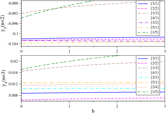
FIG. 1.: (Color on-line) Non-defective four-, five, and six-loop PBL approximants for the RG dimension $y_{4}$ for $n=2,3$.

Finally, let us consider the fourth-harmonic exponent. It has been shown in Refs. [55, 8] that the RG dimension $y_{4}$ is related to the exponent characterizing the stability of the O($n$) fixed point against cubic anisotropy. Thus we can use the six-loop series of the cubic model [56] to obtain the pseudo-$\epsilon$ expansion

$$y_{4} = 1-\frac{12}{n+8}\tau+\frac{4(680+62\,n+23\,n^{2})}{27(8+n)^{3}}\tau^{2}$$ (22)

$$+ \frac{-5200.56-777.127\,n+33.2649\,n^{2}+35.7448\,n^{3}+1.25111\,n^{4}}{(n+8)^{5}}\tau^{3}$$ (23)

$$+ \frac{328835.+90677.3\,n+10871.8\,n^{2}+1595.82\,n^{3}+446.805\,n^{4}+28.9975\,n^{5}+0.574653\,n^{6}}{(n+8)^{7}}\tau^{4}$$ (24)

$$+ \frac{-3.06135\,{10}^{7}-1.35901\,{10}^{7}\,n-2.55849\,{10}^{6}\,n^{2}-179042.\,n^{3}+24766.4\,n^{4}+8290.96\,n^{5}+672.157\,n^{6}+22.2622\,n^{7}+0.318104\,n^{8}}{(n+8)^{9}}\tau^{5}$$ (25)

$$+ \left[\frac{3.18214\,{10}^{9}+1.83869\,{10}^{9}\,n+4.52163\,{10}^{8}\,n^{2}+5.94633\,{10}^{7}\,n^{3}+5.79335\,{10}^{6}\,n^{4}+913345.\,n^{5}+161861.\,n^{6}+14567.2\,n^{7}}{(n+8)^{11}}\right.$$ (27)

$$\left.\frac{+669.512\,n^{8}+17.0980\,n^{9}+0.199456\,n^{10}}{(n+8)^{11}}\right]\tau^{6}.$$

From a general analysis [1, 8], it is known that $y_{4}$ is positive for $n>N_{c}$ and negative in the opposite case, with $N_{c}$ a bit smaller than $3$ [1]. The series (27) is alternating in signs for $n\lesssim 5$. However, in this case, the coefficients are not so small for a simple Padé summation to be effective. Thus, we apply a PBL resummation. Fig. 1 sketches the non-defective PBL approximants for $n=2,3$. It is evident that several approximants are very close to each other, whereas the $[1/M]$ ones are well separated. Usually, when facing with a similar situation, the PBL approximants that are far from the mean-value are discarded in the averaging procedure. Since in this case we may not take advantage of the Padé data, in order to be sure to not underestimate the error, we report in Table IV two different estimates: one is the average over all PBL (which we will term “safe”), the other (“best”) is obtained discarding the $[1/M]$ approximants. For $n=5,16$ we report only the “safe” estimate, because we do not have anymore evidence for a trend in the $[1/M]$ approximants.

IV Conclusions

In this paper we determined the critical exponents associated with harmonic operators of degree 2, 3, and 4 in O($n$) models by means of pseudo-$\epsilon$ expansion. All our results for $y_{i}$, $\phi_{i}$, $\gamma_{i}$, and $\beta_{i}$ are reported for $n=$ 0, 1, 2, 3, 4, 5, and 16 in Table IV.

TABLE IV.: Final estimates from six-loop pseudo-$\epsilon$ expansion. The values of $y_{i}$ are calculated directly from the series reported in the text. Whereas $\phi_{i}$, $\gamma_{i}$, and $\beta_{i}$ are obtained by means of scaling laws, using the most accurate theoretical estimates for standard critical exponents [54] with our Padé final results of the RG dimension $y_{i}$.

	$n=0$	$n=1$	$n=2$	$n=3$	$n=4$	$n=5$	$n=16$
$y_{2}$ (PBL)	-	1.7348(2)	1.7645(3)	1.7897(3)	1.8112(6)	1.830(1)	-
$y_{2}$ (Padé)	-	1.733(6)	1.763(4)	1.789(3)	1.811(2)	1.830(2)	1.927(4)
$\phi_{2}$	1	1.092(4)	1.184(3)	1.272(2)	1.356(4)	1.398(4)	1.755(4)
$\beta_{2}$	-	0.798(4)	0.831(3)	0.861(2)	0.891(3)	0.894(3)	0.978(4)
$\gamma_{2}$	-	0.294(8)	0.353(5)	0.411(4)	0.466(3)	0.504(3)	0.778(7)
$y_{3}$ (PBL)	0.7258(2)	0.8153(3)	0.8920(2)	0.956(2)	1.011(2)	1.059(4)	-
$y_{3}$ (Padé)	0.725(30)	0.814(10)	0.891(9)	0.957(4)	1.014(4)	1.063(7)	1.31(1)
$\phi_{3}$	0.426(18)	0.513(6)	0.598(6)	0.681(3)	0.759(4)	0.812(6)	1.19(1)
$\beta_{3}$	1.336(18)	1.377(6)	1.416(6)	1.453(3)	1.488(5)	1.480(7)	1.54(1)
$\gamma_{3}$	-0.91(4)	-0.865(13)	-0.818(12)	-0.772(6)	-0.728(6)	-0.668(11)	-0.35(2)
$y_{4}$ safe	-0.380(18)	-0.23(1)	-0.098(6)	0.012(6)	0.104(8)	0.188(8)	0.62(1)
$y_{4}$ best	-0.393(5)	-0.236(3)	-0.103(1)	0.0094(30)	0.107(5)

In order to make a comparison with the values in the literature we report in Table V all the most accurate theoretical estimates for $y_{i}$, as obtained by means of scaling relations (4) using the most precise determinations of standard critical exponents [54]. For all values of $n$ our estimates are in perfect agreement with all known results and in the majority of the cases they are the most precise ones. We stress that such high accurateness should not be due to underestimation of the uncertainty, since we check our final error bars with other resummation techniques, such as Padé-Borel-Leroy and conformal mapping. However the large $n$ results need to be discussed, since our estimates for $n\gtrsim 6$ can be affected by systematic errors, because the perturbative series we summed have not alternating signs. Anyway, for $n=16$ all the theoretical estimates are in good agreement, signaling that the evaluation of our uncertainty is probably good even in this case.

TABLE V.: Theoretical estimates of the RG dimension $y_{i}$ as obtained by various approaches for several $n$: five-loop $\epsilon$ expansion ($\epsilon$ exp), six-loop fixed-dimension expansion (FD), high-temperature expansion (HT exp), Monte Carlo simulations (MC), and $1/n$ expansion at order $O(1/n^{2})$ or $O(1/n)$. The results are obtained by using scaling relations, using the most precise theoretical estimates for standard critical exponents [54].

$y_{2}$		$n=1$	$n=2$	$n=3$	$n=4$	$n=5$	$n=16$
6-loop (pseudo-$\epsilon$)		1.733(6)	1.763(4)	1.789(3)	1.811(2)	1.830(2)	1.927(4)
6-loop (FD) [24]			1.763(18)	1.787(30)	1.80(5)	1.83(5)	1.92(6)
5-loop ($\epsilon$-exp) [8]			1.766(6)	1.790(3)	1.813(6)	1.832(8)
MC [42]			1.755(3)	1.787(3)	1.812(2)
MC [44]						1.815(39)
HT exp. [9]			1.750(22)	1.758(21)
O($1/n$) [57]				1.640	1.730	1.784	1.932
O($1/n^{2}$) [46, 58]				1.78(14)	1.83(6)	1.88(2)	1.95(3)
$y_{3}$	$n=0$	$n=1$	$n=2$	$n=3$	$n=4$	$n=5$	$n=16$
6-loop (pseudo-$\epsilon$)	0.725(30)	0.814(10)	0.891(9)	0.957(4)	1.014(4)	1.063(7)	1.31(1)
6-loop (FD)[34]	0.758(19)		0.895(15)	0.953(23)	1.015(31)	1.065(19)	1.310(13)
5-loop ($\epsilon$-exp) [34]	0.739(9)		0.892(22)	0.958(42)	1.020(45)	1.064(25)	1.28(10)
O($1/n$) [57]					0.791	0.933	1.323
$y_{4}$	$n=0$	$n=1$	$n=2$	$n=3$	$n=4$	$n=5$	$n=16$
6-loop (pseudo-$\epsilon$) best	-0.393(5)	-0.236(3)	-0.103(1)	0.0094(30)	0.107(5)
6-loop (pseudo-$\epsilon$) safe	-0.380(18)	-0.23(1)	-0.098(6)	0.012(6)	0.104(8)	0.188(8)	0.62(1)
6-loop (FD) [56, 55]			-0.103(8)	0.013(6)	0.111(4)	0.189(10)
5-loop ($\epsilon$-exp) [56, 8]			-0.114(4)	0.003(4)	0.105(6)	0.198(11)
MC Ref. [43]			-0.17(2)	-0.0007(29)	0.130(24)
O($1/n$) [57]						-0.08	0.662

Let us finally compare our values with some experiments. We mention the result $\phi^{n=2}_{2}=1.17(2)$ for the ($2\rightarrow 1+1$) bicritical point in GdAlO₃ [59], and $\phi^{n=3}_{2}=1.279(31)$ in the ($3\rightarrow 2+1$) study of MnF₂ [60]. Other experimental measures of $\phi_{2}$ can be found in Ref. [61]. The experimental results obtained for a nematic-smectic-A transition reported in Ref. [22] are $\beta_{2}^{n=2}=0.76(4)$ and $\gamma_{2}^{n=2}=0.41(9)$. For the third harmonic exponent we quote $\beta_{3}^{n=2}\simeq 1.66$ in liquid crystals [23], $\beta_{3}^{n=2}=1.50(4)$ (Ref. [32]) $\beta_{3}^{n=2}=1.80(5)$ (Ref. [30]) in Rb₂ZnCl₄. All these values compare well (within their own uncertainties) with our results.

REFERENCES

- [1] A. Pelissetto and E. Vicari, Phys. Rep. 368 (2002) 549 [cond-mat/0012164].
- [2] F. J. Wegner, Phys. Rev. B 6, 1891 (1972).
- [3] D. J. Wallace and R. K. P. Zia, J. Pys. C 8, 839 (1975).
- [4] For general reviews see P. Calabrese, A. Pelissetto, and E. Vicari in Frontiers in Superconductivity Research ed B P Martins (Nova Science, Hauppage, New York, 2004) [cond-mat/0306273]; P. Calabrese, A. Pelissetto, P. Rossi, and E. Vicari Int. J. Mod. Phys. B 17 5829 (2003) [hep-th/0212161].
- [5] M. E. Fisher and P. Pfeuty, Phys. Rev. B 6, 1889 (1972).
- [6] M. E. Fisher and D. Nelson, Phys. Rev. Lett. 32, 1350 (1974).
- [7] A. Aharony, in Phase Transitions and Critical Phenomena, edited by C. Domb and J. L. Lebowitz (Academic Press, New York, 1976), Vol. 6, p. 357.
- [8] P. Calabrese, A. Pelissetto and E. Vicari, Phys. Rev. B 67, 054505 (2003) [cond-mat/0209580].
- [9] P. Pfeuty, D. Jasnow, and M. E. Fisher, Phys. Rev. B 10, 2088 (1974).
- [10] M. E. Fisher, Phys. Rev. Lett. 34, 1634 (1975).
- [11] J. M. Kosterlitz, D. R. Nelson, and M. E. Fisher, Phys. Rev. Lett. 33, 813 (1974); Phys. Rev. B 13, 412 (1976).
- [12] G. Aeppli and V.J. Emery, Proc. Natl. Acad. Sci. USA 98, 11903 (2001).
- [13] S.-C. Zhang, Science 275, 1089 (1997).
- [14] E. Dagotto, J. Burgy, and A. Moreo, cond-mat/0209689. For an introduction to the subject see e.g. E. Dagotto, Phase Separation and Colossal Magnetoresistance, (Springer-Verlag, Berlin, 2002).
- [15] S. Chandrasekharan, V. Chudnovsky, B. Schlittgen, and U.-J. Wiese, Nucl. Phys. B (Proc. Suppl.) 94, 449 (2001) [hep-lat/0011054]; S. Chandrasekharan and U.-J. Wiese, hep-ph/0003214; F. Sannino and K. Tuominen, Phys. Rev. D 70, 034019 (2004) [hep-ph/0403175].
- [16] R. R. Netz and A. Aharony, Phys. Rev. E 55, 2267 (1997).
- [17] For a general review, see J. D. Litster and R. J. Birgeneau, Phys. Today 35, No. 5, 261 (1982), and E. Fawcett, Rev. Mod. Phys. 60, 1 (1988).
- [18] A. Aharony, R. J. Birgeneau, J. D. Brock, and J. D. Litster, Phys. Rev. Lett. 57, 1012 (1986).
- [19] S. Girault, A. H. Moudden, and J. P. Pouget, Phys. Rev. B 39, 4430 (1989).
- [20] J. D. Brock, D. Y. Noh, B. R. McClain, J. D. Litster, R. J. Birgeneau, A. Aharony, P. M. Horn, and J. C. Liang, Z. Phys. B 74, 197 (1989).
- [21] C. W. Garland, G. Nounesis, M. J. Young, and R. J. Birgeneau, Phys. Rev. E 47, 1918 (1993).
- [22] L. Wu, M. J. Young, Y. Shao, C. W. Garland, R. J. Birgeneau, and G. Heppke, Phys. Rev. Lett. 72, 376 (1994).
- [23] A. Aharony, R. J. Birgeneau, C. W. Garland, Y.-J. Kim, V. V. Lebedev, R. R. Netz, and M. J. Young, Phys. Rev. Lett. 74, 5064 (1995).
- [24] P. Calabrese, A. Pelissetto and E. Vicari, Phys. Rev. E 65, 046115 (2002) [cond-mat/0111160].
- [25] P. Calabrese and A. Gambassi, JSTAT 0407, P013 (2004) [cond-mat/0406289].
- [26] J. F. Fernández, Phys. Rev. B 38, 6901 (1988).
- [27] A. Aharony, Phys. Rev. B 12, 1038 (1975); P. Calabrese, A. Pelissetto and E. Vicari, Phys. Rev. E 70, 036104 (2004) [cond-mat/0311576]; M. Dudka, R. Folk, Yu. Holovatch, cond-mat/0406692.
- [28] S. Sachdev and T. Morinari, Phys. Rev. B 66, 235117 (2002).
- [29] P. Calabrese, A. Pelissetto, and E. Vicari, cond-mat/0408130; A. Pelissetto and E. Vicari, hep-th/0409214.
- [30] S. R. Andrews and H. Mashiyama, J. Phys. C 16, 4985 (1983).
- [31] G. Helgesen, J. P. Hill, T. R. Thurston, and D. Gibbs, Phys. Rev. B 52, 9446 (1995).
- [32] M. P. Zinkin, D. F. McMorrow, J. P. Hill, R. A. Cowley, J.-G. Lussier, A. Gibaud, G. Gr bel, and C. Sutter, Phys. Rev. B 54, 3115 (1996).
- [33] A. Aharony, K. A. Müller, and W. Berlinger, Phys. Rev. Lett. 38, 33 (1977).
- [34] M. De Prato, A. Pelissetto and E. Vicari, Phys. Rev. B 68, 092403 (2003) [cond-mat/0302145].
- [35] G. R. Golner, Pys. Rev. B 8, 3419 (1973); D. Amit and A. Shcherbakov, J. Phys. C 7, l96 (1974); R. K. P. Zia and D. J. Wallace, J. Phys. A 9, 1495 (1975); D. Amit, J. Phys. A 9, 144 (1976).
- [36] D. Mukamel, M. E. Fisher, and E. Domany, Phys. Rev. Lett. 37, 565 (1976).
- [37] B. Nienhuis, Phys. Rev. Lett. 49, 1062 (1982); J. Stat. Phys. 34, 731 (1984).
- [38] K. G. Wilson, Phys. Rev. Lett. 28, 548 (1972); A. Houghton and F. J. Wegner, Phys. Rev. A 10, 435 (1974).
- [39] Y. Yamazaki, Phys. Lett. 49A, 215 (1974).
- [40] J. E. Kirkham, J. Phys. A 14 L437 (1981).
- [41] H. Kleinert and V. Schulte-Frohlinde, Phys. Lett. B 342, 284 (1995) [cond-mat/9503038]; H. Kleinert, S. Thoms and V. Schulte-Frohlinde, Phys. Rev. B 56, 14428 (1997) [quant-ph/9611050].
- [42] H. G. Ballesteros, L. A. Fernandez, V. Martin-Mayor and A. Munoz Sudupe, Phys. Lett. B 387, 125 (1996) [cond-mat/9606203].
- [43] M. Caselle and M. Hasenbusch, J. Phys. A 31, 4603 (1998) [cond-mat/9711080].
- [44] X. Hu, Phys. Rev. Lett. 87, 057004 (2001).
- [45] S. Hikami and R. Abe, Prog. Theor. Phys. 52, 369 (1974); R. Oppermann, Phys. Lett. A 47, 383 (1974).
- [46] J. A. Gracey, Phys. Rev. E 66, 027102 (2002) [cond-mat/0206098].
- [47] The pseudo- expansion was introduced by B. G. Nickel, see citation 19 in Ref. [48].
- [48] J. C. Le Guillou and J. Zinn-Justin, Phys. Rev. B 21, 3976 (1980).
- [49] R. Guida and J. Zinn-Justin, J. Phys. A 31, 8103 (1998) [cond-mat/9803240].
- [50] C von Ferber and Yu. Holovatch, Europhys. Lett. 39, 31 (1997); Phys. Rev. E 56, 6370 (1997); Phys. Rev. E 59 6914; Phys. Rev E 65 042801.
- [51] R. Folk, Yu. Holovatch, and T. Yavors’kii, Phys. Rev. B 62, 12195 (2000); B 63, 189901(E) (2001).
- [52] M. Dudka, Yu. Holovatch, and T. Yavors’kii, Acta Phys. Slov. 52 (2002) 323; J. Phys. A 37, 10727 (2004); Yu. Holovatch, M. Dudka, and T. Yavors’kii, J. Phys. Studies 5 (2001) 233; P. Calabrese and P. Parruccini, Nucl. Phys. B 679, 568 (2004) [cond-mat/0308037]; Yu. Holovatch, D. Ivaneyko, and B. Delamotte, J. Phys. A 37, 3569 (2004) [cond-mat/0312260]; P. Calabrese and P. Parruccini, JHEP 0405, 018 (2004) [hep-ph/0403140]; P. Calabrese, E. V. Orlov, D. V. Pakhnin and A. I. Sokolov, Phys. Rev. B 70, 094425 (2004) [cond-mat/0405432].
- [53] S. A. Antonenko and A. I. Sokolov, Phys. Rev. E 51, 1894 (1995) [hep-th/9803264].
- [54] For the standard exponents we have taken the following numerical results: for [T. Prellberg, J. Phys. A 34, L599 (2001)] and [S. Caracciolo, M. S. Causo, and A. Pelissetto, Phys. Rev. E 57, 1215(R) (1998)], for [M. Campostrini, A. Pelissetto, P. Rossi, and E. Vicari, Phys. Rev. E 65, 066127 (2002)] for [M. Campostrini, M. Hasenbusch, A. Pelissetto, P. Rossi, and E. Vicari, Phys. Rev. B 63, 214503 (2001)], for [M. Campostrini, M. Hasenbusch, A. Pelissetto, P. Rossi, and E. Vicari, Phys. Rev. B 65, 144520 (2002)], for [M. Hasenbusch, J. Phys. A 34, 8221 (2001)] for [A. Butti and F. Parisen Toldin, Nucl. Phys. B 704, 527 (2005)], and for (Ref. [53]). In three dimensions is given by the scaling law . Other numerical estimates can be found in Ref. [1].
- [55] P. Calabrese, A. Pelissetto and E. Vicari, cond-mat/0203533.
- [56] J. M. Carmona, A. Pelissetto and E. Vicari, Phys. Rev. B 61, 15136 (2000) [cond-mat/9912115].
- [57] From Ref. [3], taking into account the scaling relation one gets the result .
- [58] In Ref. [46] were reported the four different estimates for , , , and as obtained by Padé-Borel analysis of the corresponding expansions. These four estimates obviously leads to different estimates of . The value in the Tab. V is the average of the four as obtained by means of scaling relations (for the exponent we take the value in [54]) and the uncertainty is the maximum deviation. Obviously, the quoted error bars are only indicative.
- [59] H. Rohrer and Ch. Gerber, Phys. Rev. Lett. 38, 909 (1977).
- [60] A. R. King and H. Rohrer, Phys. Rev. B 19, 5864 (1979).
- [61] V. Privman, P. C. Hohenberg, and A. Aharony, in Phase Transitions and Critical Phenomena, edited by C. Domb and J. L. Lebowitz (Academic Press, New York, 1991), Vol. 14.