Quasi-stationary trajectories of the HMF model: a topological perspective

Abstract

We employ a topological approach to investigate the nature of quasi-stationary states of the Mean Field XY Hamiltonian model that arise when the system is initially prepared in a fully magnetized configuration. By means of numerical simulations and analytical considerations, we show that, along the quasi-stationary trajectories, the system evolves in a manifold of critical points of the potential energy function. Although these critical points are maxima, the large number of directions with marginal stability may be responsible for the slow relaxation dynamics and the trapping of the system in such trajectories.

The so called Mean Field $XY$ Hamiltonian Model (HMF model) Antoni has received great attention during the last years in the statistical mechanics community, mainly because of the richness of its dynamical behavior Latora01a ; anteneodo ; all ; Montemurro ; Pluchino ; yamaguchi ; superdif . The model is defined by a set of $N$ particles, or rotators, moving on a unitary circle. The dynamics of the system is ruled by the following Hamiltonian:

$${\cal H}=\frac{1}{2}\sum_{i=1}^{N}p_{i}^{2}+\frac{1}{2N}\sum_{i,j=1}^{N}[1-\cos{(\theta_{i}-\theta_{j})}]\,.$$ (1)

Here $\theta_{i}$ represents the rotation angle of the $i$-th particle (with $\theta_{i}\in(0,2\pi])$ and $p_{i}$ its conjugate momentum. This model can be considered as a kinetic version of the mean field $XY$ magnetic model with ferromagnetic interactions. From a thermodynamical point of view the model is extremely simple, in contrast to its rich and still not well understood dynamical behavior. On one side, being a mean field model, its equilibrium thermodynamics can be exactly solved in the canonical ensemble, yielding a second order ferromagnetic phase transition. On the other side its relaxational dynamics is very complex and equilibrium is not easily attained from an important set of initial conditions yamaguchi ; superdif ; hmf . The origin of this kinetic complexity is elusive and some similarity with the phenomenology of disordered systems has been advocated Montemurro ; Pluchino . Nevertheless, the existence of this relation is not at all obvious. In first place, there is no imposed disorder on the Hamiltonian. Second, the couplings are all ferromagnetic, avoiding in this case any kind of structural frustration. Finally, the infinite range of the interactions further simplifies both the dynamics and the thermodynamics of the model, avoiding any topological consideration on the structure of the lattice where particles are located. On the other hand, and also due to the infinite range of the interactions, its dynamics can be efficiently integrated in computer simulations. Therefore, this is an excellent prototype for analyzing the microscopic dynamics of a finite system close to a critical point.

The microcanonical simulations of the HMF reproduce many of the anomalous critical behaviors observed in nuclear and cluster fragmentation processes. In particular, depending on the initial preparation of the system, it is possible to verify the existence of negative specific heat curves, qualitatively similar to those observed in recent fragmentation experiments in small clusters (see for instance experiment and references therein). But the interest on this model largely exceeds this motivation. The existence of quasi-stationary solutions whose life-times diverge Latora01a ; yamaguchi , in the thermodynamical limit $N\to\infty$, has raised the question on whether it is possible or not to construct a measure theory able to predict the stationary values of physical observables in long standing out of equilibrium regimes Tsallis88 . Furthermore, the existence of a glassy-like relaxation dynamics Montemurro ; Pluchino along quasi–stationary trajectories, has opened new challenging questions on the origin of such unexpected behavior for an unfrustrasted non disordered model. Finally, in the last few years, the HMF model has been used, as a paradigmatic example, for the study of the so called Topological Hypothesis geometric ; Casetti03 ; theorem which asserts that phase transitions, even in a finite system, can be identified by searching for drastic topological changes in the submanifolds of the interaction potential.

Concerning the HMF thermodynamics Antoni , the usual microcanonical and canonical calculations predict that the system suffers a second order phase transition at $T_{c}=1/2$ (which corresponds to an internal energy per particle $U_{c}/N=3/4$), from a low temperature ordered phase to a high temperature disordered one. Actually, one can associate to each rotator a local magnetization: $\vec{m}_{i}=(\cos{\theta_{i}},\sin{\theta_{i}}),$ and then define the order parameter of the transition as the global magnetization:

$$\vec{M}=(M_{x},M_{y})=\frac{1}{N}\sum_{i}\vec{m}_{i}.$$ (2)

At the critical energy, $M\equiv|\vec{M}|$ vanishes continuously as the system is heated from the ordered phase.

Concerning the dynamics, when the system is prepared very far from equilibrium, for energies just below the critical one, the system gets trapped into quasi-equilibrium trajectories. These trajectories are characterized by time averages of one-time observables which reach, after a rapid initial transient, almost constant values which do not coincide with those predicted by microcanonical or canonical ensemble calculations Latora01a . The average time that a system of size $N$ remains in a quasi–stationary trajectory grows with $N$ Latora01a ; yamaguchi . Therefore, if the system were infinite, it would remain there forever, without ever reaching true equilibrium. An even more surprising scenario appears when one considers the relaxation of the two–time correlation function $C(t,t^{\prime})$ (either in the whole phase space Montemurro or considering only the momenta space Pluchino ). The explicit dependence of $C$ on both times $t$ and $t^{\prime}$ indicates the loss of time–translational invariance, proper of equilibrium states, and the appearance of memory effects, a phenomenon usually called aging. The scaling law of the two–time autocorrelation functions Montemurro ; Pluchino is qualitatively similar to that observed in some real spin glasses Vincent02 . Nevertheless we will show that the physical mechanisms behind the quasi-stationary states of the HMF are completely different from those present in disordered systems.

In this work we will show, through numerical simulations, that the complex nonequilibrium quasi–stationary regime observed just below the critical energy can be interpreted from a topological point of view. Our analysis will focus on the topology of the surface defined by the potential energy in the configuration space. The HMF potential energy, as well as any Curie-Weiss like potential, can be written in terms of the order parameter of the system:

$$V=\frac{N}{2}(1-M^{2})\;.$$ (3)

Note that the potential energy per particle $V/N$ takes values in the interval $0\leq V/N\leq v_{c}\equiv 1/2$. The lower limit corresponds to the case of the fully ordered configurations (hence $M=1$) and the upper bound to a completely disordered configuration. The configuration space manifold $\cal M$ is an $N$-dimensional torus parametrized by the $N$ angles $\theta_{i}$. The critical points (CPs) of $\cal M$ are those points for which all the $N$ derivatives of $V/N$ vanish, i.e., ${\partial(V/N)}/{\partial\theta_{i}}=0$, for $i=1,\ldots,N$. Making use of the infinite range of the interactions, one can write the derivatives of the potential in terms of the two components of the order parameter, namely,

$$\frac{\partial V/N}{\partial\theta_{i}}=\frac{1}{N}M_{x}\sin{\theta_{i}}-\frac{1}{N}M_{y}\cos{\theta_{i}}=0\;.$$ (4)

Furthermore, CPs can be classified according to the eigenvalues of the Hessian of $V/N$, that for the HMF can be written as $\bf H=D+B$ Casetti03 , where

$$B_{ij} = -\frac{1}{N^{2}}\ (1-\delta_{ij})\ \cos({\theta_{i}-\theta_{j}})-\frac{1}{N^{2}}\ \delta_{ij}\,,$$

$$D_{ij} = \frac{\delta_{ij}}{N}\ (M_{x}\cos{\theta_{i}}+M_{y}\sin{\theta_{i}})\,.$$ (5)

In our work we use the following protocol: starting from a far-from-equilibrium configuration, we integrate numerically the set of Hamilton equations of the system using a fourth order symplectic method with a very small time step (typically $dt=0.01$). Along the trajectories we evaluate, at each time step, the modulus of the $N$ derivatives of $V/N$ given by (4) and identify the maximum over $i=1,\ldots,N$, through

$$\lambda=N\max_{i}\left|\frac{\partial(V/N)}{\partial\theta_{i}}\right|\,.$$ (6)

Then, each time that $\lambda=0$, it means that the system reaches a CP (actually, due to the finiteness of time step, $\lambda$ is never exactly zero, but it gets closer as $dt$ decreases).

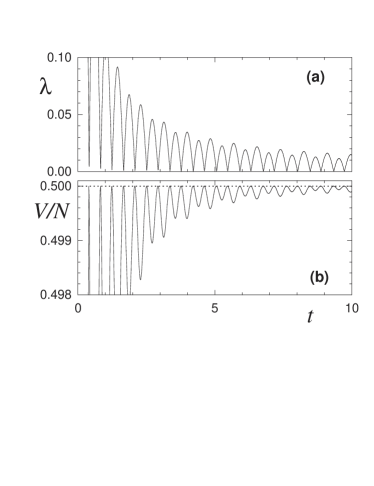
Let us first analyze the behavior of the system in the disordered phase. It is important to stress that, although the system ultimately relaxes to equilibrium, a slow relaxation has been observed when starting very far from equilibrium superdif . This is probably due to the fact that rotators move almost freely and trajectories are weakly chaotic anteneodo ; lyaps . In Fig. 1, we plot $V/N$ and $\lambda$ as a function of $t$, for $U/N=10$, in the disordered phase well above the critical energy $U_{c}/N=3/4$. The system has been initially prepared in a “water-bag” configuration, with all the rotators aligned along the $x$ axis ($\theta_{i}=0$, for all $i$) and the momenta drawn from a uniform distribution (actually we used regularly spaced momenta vlasov ). Fig. 1 indicates that the system periodically visits CPs of the potential, corresponding to $V/N=1/2$ (hence $M=0$). In fact the observed period is of the order of the mean period of rotation lyaps .

Figure 1: Time evolution of (a) $\lambda$, the largest modulus of the derivatives of $V$, and (b) $V/N$, the potential energy per particle, for a system of $500$ particles and $U/N=10$, well above the phase transition. The system was initially prepared in a regular water-bag configuration. The dotted line in (b) corresponds to the equilibrium value in the thermodynamic limit.

Figure 2: Time evolution of $\lambda$ (a) and $V/N$ (b) for a system of $500$ particles and $U/N=0.69$, just below the phase transition. The system was initially prepared in a regular water-bag configuration. The dotted and dashed lines in (b) correspond to equilibrium and metaequilibrium values in the thermodynamic limit, respectively.

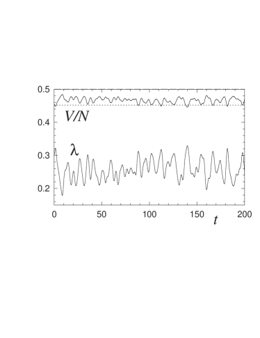
Let us now compare these results with those obtained in the low energy phase, just below the phase transition. In this case, quasi-stationary solutions emerge, displaying a kind of glassy-like dynamics characterized by weak chaos, non-Gaussian velocity distributions and sub–aging, as mentioned above. In Fig. 2, we plot $V/N$ and $\lambda$ vs. $t$ for $U/N=0.69$ and water-bag initial conditions. Here we verify that again the system sequentially visits one CP of the potential energy after another, also corresponding to $M=0$. However, at variance with the high energy phase, the time intervals $\Delta\tau$ elapsed between two successive CPs do not present any pattern of periodicity. On the contrary, the system visits the CPs in an apparently disordered way. The probability distribution function (PDF) $P(\Delta\tau)$ of time intervals between CPs is shown in Fig. 3. $P(\Delta\tau)$ can be reasonably fitted by a power law decay. Other striking features of the dynamical behavior can be noted in Fig. 2. First, the system is initialized in a configuration at the bottom of the potential energy $V/N=0$ and it goes almost abruptly to a region with a mean potential energy per particle larger than the equilibrium mean potential energy, and stays around this level during the whole time span of the simulation. In fact it goes close to the top of the potential energy landscape, $V/N\approx 1/2$, tries to escape downhill but uses the kinetic energy gain to attain again CPs at the top. Somehow the system is not able to relax from this level to the equilibrium level during very large time scales. The configurations sampled correspond to the quasi-stationary states and the system stays there during time spans which scale with the size N, being trapped forever in the thermodynamic limit. One can say that, in configuration space, quasi-stationary states are always near CPs of the landscape.

Figure 3: Probability distribution function $P(\Delta\tau)$ of the time intervals between two consecutive critical points, for the same system of Fig. 2.

We next address the effect of system size. The same qualitative behavior can be observed, with a bigger numerical effort, for larger systems. The departure from the CPs (measured by the height of $\lambda$ between consecutive CPs) decreases as $N$ increases, but the distribution of $\Delta\tau$ remains unaltered. From Eqs. (3) and (4), it is straightforward to see that at the critical level $v_{c}=1/2$ the CPs are continuously degenerate. Consequently as N grows and fluctuations outside the critical level diminish the system wanders more and more inside this manifold of CPs. As the energy decreases, the CPs are visited more sparsely, down to $U/N\approx 0.67$, where the system stops wandering among CPs. It is noteworthy that spatially homogeneous states lose Vlasov stability approximately at that energy vlasov .

Figure 4: Time evolution of $\lambda$ and $V/N$ for a system of $500$ particles and $U/N=0.69$, just below the phase transition. The system was initially prepared in a close to equilibrium configuration. The dotted line corresponds to the equilibrium value of $V/N$.

A completely different scenario emerges when the system is prepared, at a given energy, in an almost equilibrated initial configuration. The plot of $\lambda$ vs. $t$ presented in Fig. 4 clearly indicates that, in this case, the system does not wander among CPs. Its potential energy per particle (and then also its temperature) rapidly starts fluctuating around their canonical values, showing strong finite size effects.

A crucial piece of information comes from the stability of the visited CPs. Since capturing the exact time at which the dynamics passes through a CP is a difficult task, numerical evaluation of the Hessian at CPs arising from the dynamics may lead to wrong estimates. Therefore it is important to perform some analytical calculations. In order to do so, let us recall that, both in the high energy phase and in the quasi-stationary states, the CPs correspond to $V/N=1/2$ (see Figs. 1 and 2), hence they are points of $\cal M$ with zero magnetization. Moreover, the distribution of angles at those points is approximately uniform vlasov . A configuration with these characteristics for which analytical calculations are possible, consists in regularly distributed angles in the interval $(0,2\pi]$, i.e., $\theta_{k}=2\pi k/N$, $k=1,...,N$ for even $N$. If $M=0$, from Eq. (5), the Hessian of the potential energy is $\bf H=B$. Then, for the regular configuration we have

$${\bf H}={\bf B}=-\frac{1}{N^{2}}\ (\openone+{\bf A}),$$ (7)

where $A_{kl}=\cos(2\pi(k-l)/N)$. This circulant matrix can be diagonalized in Fourier space, yielding the following eigenvalues of the Hessian matrix

$$H_{l}=-\frac{1}{N^{2}}\biggl{(}\cos(\pi l)+2\sum_{r=0}^{N/2}\cos(2\pi rl/N)\cos(2\pi r/N)\biggr{)},$$ (8)

for $1\leq l\leq N$. Thus, we obtain $H_{1}=H_{N-1}=-1/(2N)$ while the remaining eigenvalues are null. This means that at these CPs there are two unstable directions and $N-2$ marginal ones. This picture remains valid for more general situations than those restricted to the particular regular cases. In fact, we have verified that when angles are randomly chosen in the interval $(0,2\pi]$ there are two eigenvalues with values close to $-1/(2N)$ and the remaining $N-2$ vanish. Finally, the eigenvalues calculated from the configurations of the dynamics very close to CPs are also consistent with this picture. >From this analysis it is clear that in the high energy phase and also in the quasi-stationary low energy states, the systems wanders in an almost flat landscape.

In the high energy phase, energy is mainly kinetic, leading to ballistic behavior in the flat landscape of CPs during long time scales. In the low energy, quasi-equilibrium regime, kinetic energy is comparable to the potential one. At this relatively low energies diffusion is slower than ballistic. Nevertheless, due to the flatness of configuration space superdiffusive behavior is observed superdif .

Summarizing, we have seen, by means of numerical simulations, that the quasi-stationary trajectories observed in the HMF model can be interpreted in terms of the topological properties of the potential energy per particle $V/N$ of the model. Starting from a far from equilibrium configuration with $V/N=0$, the system initially decreases as much as possible its kinetic energy and settles at the flat top of its potential energy. The simulations confirm that along the quasi stationary states the system wanders among different CPs with only two negative directions and $N-2$ marginal ones. Moreover, CPs at the upper critical level are continuously degenerate. This suggests that once inside this critical submanifold the system cannot go out easily and relax to equilibrium. A probable scenario in the thermodynamic limit is that, as the fluctuations of the potential energy close to the critical level $v_{c}=1/2$ go to zero, the system keeps wandering continuously inside the manifold of CPs and consequently remains forever out of thermodynamic equilibrium.

This work was partially supported by CONICET (Argentina), Agencia C rdoba Ciencia (Argentina), Secretaría de Ciencia y Tecnología de la Univ. Nac. Córdoba (Argentina) and CNPq (Brazil).

References

- (1) M. Antoni and S. Ruffo, Phys. Rev. E 52, 2361 (1995).
- (2) V. Latora, A. Rapisarda, and C. Tsallis, Phys. Rev. E 64, 056134 (2001).
- (3) C. Anteneodo and C. Tsallis, Phys. Rev. Lett. 80, 5313 (1998).
- (4) V. Latora, A. Rapisarda, and S. Ruffo, Phys. Rev. Lett. 80, 692 (1998); Physica D 131, 38 (1999); V. Latora and A. Rapisarda, Chaos, Solitons Fractals 13, 401 (2001); Physica A 305, 129 (2002); F. Tamarit and C. Anteneodo, Phys. Rev. Lett. 84, 208(2000); T. Dauxois, V. Latora, A. Rapisarda, S. Ruffo and A. Torcini, in Dynamical and thermodynamics of systems with long range interactions, T. Dauxois et al. Eds., Lecture Notes in Physics 602, Springer (2002); D.H. Zanette and M.A. Montemurro, Phys. Rev. E 67, 031105 (2003); L.G. Moyano, F. Baldovin, C. Tsallis, cond-mat/0305091; L. Sguanci, D.H.E. Gross and S. Ruffo, cond–mat/0407357.
- (5) M.A. Montemurro, F.A. Tamarit and C. Anteneodo, Phys. Rev. E 67, 031106 (2003).
- (6) A. Pluchino, V. Latora and A. Rapisarda, Physica A, 340, 187 (2004); Physica A 338, 60 (2004); Physica D 193, 315 (2004); Phys. Rev. E 69 056113 (2004).
- (7) Y.Y. Yamaguchi, Phys. Rev. E 68, 066210 (2003); Y.Y. Yamaguchi, J. Barré, F. Bouchet, T. Dauxois and S. Ruffo, Physica A 337, 36 (2004).
- (8) V. Latora, A. Rapisarda, and S. Ruffo, Phys. Rev. Lett. 83, 2104 (1999); F. Bouchet and T. Dauxois, preprint cond-mat/0407703.
- (9) P.H. Chavanis, J. Vatteville and F. Bouchet, preprint cond-mat/0408117; P.H Chavanis, preprint cond-mat/0409641.
- (10) M. Schmidt, R. Kusche, T. Hippler, J. Donges, W. Kronmüller, B. von Issendorff and H. Haberland, Phys. Rev. Lett. 86, 1191 (2001).
- (11) C. Tsallis, J. Stat. Phys. 52, 479 (1988); Nonextensive Mechanics and Thermodynamics, edited by S. Abe and Y. Okamoto, Lecture Notes in Physics Vol. 560 (Springer, Berlin, 2001); in Non-Extensive Entropy-Interdisciplinary Applications, edited by M. Gell-Mann and C. Tsallis, (Oxford University Press, Oxford, 2004).
- (12) L. Casetti, E.G.D. Cohen and M. Pettini, Phys. Rev. Lett. 82, 4160 (1999); L. Casetti, E.G.D. Cohen and M. Pettini, Phys. Rev. E 65, 036112 (2002).
- (13) L. Casetti, M. Pettini and E.G.D. Cohen, J. Stat. Phys. 111, 1091 (2003).
- (14) R. Franzosi and M. Pettini, Phys. Rev. Lett. 92, 60601, (2004); A.C. Ribeiro–Teixeira and D.A. Stariolo, Phys. Rev. E E 70, 16113 (2004).
- (15) J. Hammann, E. Vincent, V. Dupuis, M. Alba, M. Ocio and J.-P. Bouchaud, J. Phys. Soc. Jpn. 69, 206 (2000).
- (16) C. Anteneodo and R.O. Vallejos, Phys. Rev. E 65, 016210 (2002); C. Anteneodo, R.N.P. Maia and R.O. Vallejos, Phys. Rev. E 68, 036120 (2003).
- (17) C. Anteneodo and R. O. Vallejos, Physica A (2004, in press).