Full counting statistics for the Kondo dot.

Abstract

The generating function for the cumulants of charge current distribution is calculated for two generalised Majorana resonant level models: the Kondo dot at the Toulouse point and the resonant level embedded in a Luttinger liquid with the interaction parameter $g=1/2$. We find that the low–temperature non-equilibrium transport in the Kondo case occurs via tunnelling of physical electrons as well as by coherent transmission of electron pairs. We calculate the third cumulant (‘skewness’) explicitly and analyse it for different couplings, temperatures, and magnetic fields. For the $g=1/2$ set-up the statistics simplifies and is given by a modified version of the Levitov–Lesovik formula.

Since Schottky’s realisation that the shot noise in a conductor contains invaluable information about the physical properties of the charge carriers, the question about the noise spectra of different circuits became as important as the knowledge of their current–voltage characteristics Schottky (1918). The noise constitutes the second moment of the current distribution function (which is the probability of measuring a given value of the current) and is supposed to contain information about the charge of current carrying excitations at weak transmission (reflection). That is indeed the case for $S-S$ and $S-N$ junctions Muzykantskii and Khmelnitskii (1994); Cuevas and Belzig (2003); Jehl et al. (2000) but not been proven for a generic interacting model. As has been pointed out in Levitov and Reznikov (2004), the third cumulant also contains valuable information about the charge of the current carriers. Therefore it is natural to investigate the full current distribution function. This was an academic question for a very long time as even the measurement of the second cumulant remained on the frontier of experimental physics. Only after the work by Reulet and coworkers the measurement of the third cumulant became possible Reulet et al. (2003). Inspired by this remarkable achievement, the full current distribution function (more often referred to as ‘full counting statistics’ or FCS) has been theoretically analysed in recent year for a wide range of systems.

In their seminal work Levitov and Lesovik (1993), Levitov and Lesovik derived the exact formula for the FCS for the electron tunneling set–up (single channel):

$$\ln\chi_{0}(\lambda;V;\{T(\omega)\})={\cal T}\,\int_{-\infty}^{\infty}\frac{d\omega}{2\pi}\ln\Big{\{}1+T(\omega)$$

$$\times \big{[}n_{L}(1-n_{R})(e^{i\lambda}-1)+n_{R}(1-n_{L})(e^{-i\lambda}-1)\big{]}\Big{\}}\,,$$

where ${\cal T}$ is the waiting time, $\lambda$ is the measuring field (we will explain this notation in more detail shortly), $n_{R(L)}(\omega)=n_{F}(\omega\pm V/2)$ are the electron filling factors in the (right and left) leads, $V$ is the bias voltage, and $T(\omega)$ is the single electron transmission coefficient. The knowledge of $T(\omega)$ thus fully defines the FCS for non-interacting systems.

While the Levitov–Lesovik approach can be relatively easily generalised to various multi–terminal (multi–channel) set–ups, it is notoriously difficult to include electron–electron interactions. Up to now most works in this direction relied upon various perturbative expansions, in the tunnelling amplitude Bagrets and Nazarov (2003); Levitov and Reznikov (2004) or in the interaction strength Kindermann and Nazarov (2003) (for a recent review see Levitov (2003)), as well as calculations at zero temperature Saleur and Weiss (2001). Certainly no paradigm for an interacting FCS emerged as of yet. Notable exceptions are the contribution Safi and Saleur (2004) as well as recent works by Andreev and Mishchenko and Kindermann and Trauzettel Andreev and Mishchenko (2001); Kindermann and Trauzettel (2004), where the exact FCS was calculated for the (single–channel) Coulomb Blockade (CB) set–up of Matveev and Furusaki Matveev (1995); Furusaki and Matveev (1995). We shall establish the precise connection of these works to our results.

The purpose of this Letter is to contribute to our understanding of interacting FCSs by means of obtaining the exact FCS for two particular experimentally relevant set–ups: the Kondo dot and the resonant tunneling (RT) between two $g=1/2$ Luttinger liquids (LL).

We start with a brief description of the method. Our goal is the calculation of the generating function $\chi(\lambda)=\sum e^{iq\lambda}P_{q}$ for the probabilities $P_{q}$ of $q$ electrons being transmitted through the system over time ${\cal T}$. We first define operators $T_{i}$ transferring one electron through the system in the direction of the current ($i=R$) and in the reversed direction ($i=L$). The electron counting operator on the Keldysh contour $C$ can then be written down in its canonical form as Levitov and Lesovik (1993)

$$T_{\lambda}=e^{i\lambda(t)/2}\,T_{R}+e^{-i\lambda(t)/2}\,T_{L}\;,$$

where the measuringing field $\lambda(t)$ is explicitly time dependent, $\lambda(t)=\lambda\theta(t)\theta({\cal T}-t)$ on the forward path and $\lambda(t)=-\lambda\theta(t)\theta({\cal T}-t)$ on the backward path. According to Levitov and Lesovik (1993); Levitov and Reznikov (2004), the generating function is then given by the expectation value

$$\chi(\lambda)=\left\langle T_{{\rm C}}\,e^{-i\int\limits_{{\rm C}}T_{\lambda}(t)dt}\right\rangle\;.$$ (2)

In order to calculate $\chi(\lambda)$ we define a more general functional $\chi[\lambda_{-}(t),\lambda_{+}(t)]$ formally given by the same Eq. (2) but where $\lambda(t)$ is now understood to be an arbitrary function on the Keldysh contour, $\pm$ referring to two different functions on the time and anti-time ordered halves of the contour. Next we assume that both $\lambda_{\pm}(t)$ change slowly in time. Then, neglecting switching effects, one obtains at large ${\cal T}$

$$\chi[\lambda_{-}(t),\lambda_{+}(t)]=\exp\left\{-i\int\limits_{0}^{{\cal T}}{\cal U}[\lambda_{-}(t),\lambda_{+}(t)]dt\right\}\,,$$ (3)

where ${\cal U}(\lambda_{-},\lambda_{+})$ is the adiabatic potential. Once the adiabatic potential is computed, the statistics is recovered from $\ln\chi(\lambda)=-i{\cal T}{\cal U}(\lambda,-\lambda)$. As $\lambda_{\pm}$ are external parameters, performing the derivative of both (3) and (2) with respect to, say, $\lambda_{-}$, with help of the Feynman–Hellmann theorem Feynman (1939) we immediately obtain

$$\frac{\partial}{\partial\lambda_{-}}{\cal U}(\lambda_{-},\lambda_{+})=\left\langle\frac{\partial T_{\lambda}(t)}{\partial\lambda_{-}}\right\rangle_{\lambda}\;,$$

where we use notation

$$\langle A(t)\rangle_{\lambda}=\frac{1}{\chi(\lambda_{-},\lambda_{+})}\left\langle T_{{\rm C}}\left\{A(t)e^{-i\int\limits_{{\rm C}}T_{\lambda}(t)dt}\right\}\right\rangle\,.$$

This is somewhat more complicated than the usual Hamiltonian formalism for a quasi–stationary situation, we’ll give further technical details in the long version Komnik and Gogolin (2005); in particular, we have verified that Eq. (Full counting statistics for the Kondo dot.) comes out correctly in the non-interacting case.

In order to study the FCS for the Kondo dot we use the bosonization and refermionization approach, originally applied to this problem by Emery and Kivelson Emery and Kivelson (1992) (see also Gogolin et al. (1998)) and refined by Schiller and Hershfield (SH), see Schiller and Hershfield (1998). The starting point is the two-channel Kondo Hamiltonian (we set $\hbar=v_{F}=e=k_{B}=1$ throughout),

$$H=H_{0}+H_{J}+H_{M}+H_{V}\,,$$

where, with $\psi_{\alpha,\sigma}$ being the electron field operators in the R,L channels,

$$H_{0} = i\sum_{\alpha=R,L}\sum_{\sigma=\uparrow,\downarrow}\int\,dx\,\psi^{\dagger}_{\alpha\sigma}(x)\partial_{x}\psi_{\alpha\sigma}(x)\,,$$

$$H_{J} = \sum_{\alpha,\beta=R,L}\sum_{\nu=x,y,z}J_{\nu}^{\alpha\beta}s^{\nu}_{\alpha\beta}\tau^{\nu}\,,$$

$$H_{V} = (V/2)\sum_{\sigma}\int\,dx\,(\psi^{\dagger}_{L\sigma}\psi_{L\sigma}-\psi^{\dagger}_{R\sigma}\psi_{R\sigma})\,,$$

$$H_{M} = -\mu_{B}g_{i}H\tau^{z}=-\Delta\tau^{z}\,.$$ (4)

Here $\tau^{\nu=x,y,z}$ are the Pauli matrices for the impurity spin and ($\alpha,\beta=R,L$; $\sigma=\uparrow,\downarrow$; $\sigma^{\nu}_{\sigma\sigma^{\prime}}$ are the components of the $\nu$th Pauli matrix)

$$s^{\nu}_{\alpha\beta}=\sum_{\sigma,\sigma^{\prime}}\,\psi_{\alpha\sigma}^{\dagger}(0)\,\sigma^{\nu}_{\sigma\sigma^{\prime}}\,\psi_{\beta\sigma^{\prime}}(0)\,,$$

are the electron spin densities in (or across) the leads, biased by a finite $V$. The last term in Eq. (Full counting statistics for the Kondo dot.) stands for the magnetic field, $\Delta=\mu_{B}g_{i}H$. Following SH, we assume $J_{x}^{\alpha\beta}=J_{y}^{\alpha\beta}=J_{\perp}^{\alpha\beta}$, $J_{z}^{LL}=J_{z}^{RR}=J_{z}$ and $J_{z}^{LR}=J_{z}^{RL}=0$. The only transport process then allowed is the spin-flip tunnelling, so that we obtain for the $T_{\lambda}$ operator

$$T_{\lambda}=\frac{J_{\perp}^{RL}}{2}\left(\tau^{+}e^{i\lambda(t)/2}\psi_{R\downarrow}^{\dagger}\psi_{L\uparrow}+\tau^{-}e^{i\lambda(t)/2}\psi_{R\uparrow}^{\dagger}\psi_{L\downarrow}\right.$$

$$\left.+\tau^{+}e^{-i\lambda(t)/2}\psi_{L\downarrow}^{+}\psi_{R\uparrow}+\tau^{-}e^{-i\lambda(t)/2}\psi_{L\uparrow}^{\dagger}\psi_{R\downarrow}\right)\,.$$

After bosonization, Emery-Kivelson rotation, and refermionization (see details in Schiller and Hershfield (1998)) and going over to the Toulouse point $J_{z}=2\pi$, which is the only approximation we make, one obtains

$$H^{\prime}=H^{\prime}_{0}-i(J_{-}\,b\,\xi_{f}+J_{+}\,a\,\eta_{f})-i\Delta\,a\,b+T_{\lambda}\;,$$ (5)

where the counting term is given by

$$T_{\lambda}=-iJ_{\perp}b\,\left[\xi\,\cos(\lambda/2)-\eta\,\sin(\lambda/2)\right]\,,$$ (6)

with $J_{\pm}=(J_{\perp}^{LL}\pm J_{\perp}^{RR})/\sqrt{2\pi a_{0}}$, $J_{\perp}=J_{\perp}^{RL}/\sqrt{2\pi a_{0}}$ ($a_{0}$ is the lattice constant of the underlying lattice model) and $a$ and $b$ being local Majorana operators originating from the impurity spin. The fields $\eta_{f}$ and $\xi_{f}$ in the spin–flavour sector are equilibrium Majorana fields, whereas $\eta$ and $\xi$ in the the charge–flavour sector are biased by $V$,

$$H_{0}^{\prime} = i\int\,dx\,\Big{[}\eta_{f}(x)\partial_{x}\eta_{f}(x)+\xi_{f}(x)\partial_{x}\xi_{f}(x)$$

$$+ \eta(x)\partial_{x}\eta(x)+\xi(x)\partial_{x}\xi(x)+V\xi(x)\eta(x)\Big{]}\,.$$

Using Eqs. (5)-(Full counting statistics for the Kondo dot.) one can straightforwardly evaluate the adiabatic potential ${\cal U}(\lambda_{-},\lambda_{+})$ as the problem has become quadratic in the Majorana fields.

Skipping details of the calculation, we report the resulting exact formula for the FCS of the Kondo dot, which is the main result of this paper:

$$\ln\chi(\lambda)={\cal T}\int\limits_{0}^{\infty}\frac{d\omega}{2\pi}\ln\left\{1+T_{1}(\omega)\left[n_{L}(1-n_{R})(e^{2i\lambda}-1)+n_{R}(1-n_{L})(e^{-2i\lambda}-1)\right]\right.$$

$$\left.+T_{2}(\omega)\left[[n_{F}(1-n_{R})+n_{L}(1-n_{F})](e^{i\lambda}-1)+[n_{F}(1-n_{L})+n_{R}(1-n_{F})(e^{-i\lambda}-1)]\right]\right\}\,,$$

where now the filling factors are $n_{R,L}=n_{F}(\omega\pm V)$ [$n_{F}(\omega)$ being the conventional Fermi function], not to be confused with notation in Eq. (Full counting statistics for the Kondo dot.). The ‘transmission coefficients’ are

$$T_{1}=\frac{\Gamma_{\perp}^{2}(\omega^{2}+\Gamma_{+}^{2})}{\left[\omega^{2}-\Delta^{2}-\Gamma_{+}(\Gamma_{\perp}+\Gamma_{-})\right]^{2}+\omega^{2}(\Gamma_{+}+\Gamma_{-}+\Gamma_{\perp})^{2}}\,\,,T_{2}=\frac{2\Gamma_{\perp}\Gamma_{-}(\omega^{2}+\Gamma_{+}^{2})+2\Delta^{2}\Gamma_{\perp}\Gamma_{+}}{\left[\omega^{2}-\Delta^{2}-\Gamma_{+}(\Gamma_{\perp}+\Gamma_{-})\right]^{2}+\omega^{2}(\Gamma_{+}+\Gamma_{-}+\Gamma_{\perp})^{2}}\,\,,$$

where $\Gamma_{i}=J_{i}^{2}/2$ ($i=\pm,\perp$).

For small voltages and zero temperature the generating function turns out to be quite simple,

$$\chi(\lambda)=\left[1+T_{e}(e^{i\lambda}-1)\right]^{N}\;,$$ (9)

where $N={\cal T}V/\pi$ is the number of the incoming particles during the time interval ${\cal T}$ and $T_{e}=\sqrt{T_{1}(0)}$ is the effective transmission coefficient. We analysed explicitly the behaviour of the system around the Toulouse point. The trivialisation (9) turns out to be robust against departure from this special point in parameter space Komnik and Gogolin (2005). While (9) is the standard Levitov–Lesovik result for spinful systems, the physical content of Eq. (Full counting statistics for the Kondo dot.) is more interesting, since it cannot be reduced to binomial statistics as in Eq. (9) at finite $T$. One can see that the charge current is carried by two different quasi–particles with charges $q_{1}=2e$ and $q_{2}=e$. We identify the corresponding transmission coefficients as $T_{1}$ and $T_{2}$, respectively. It was realised by SH that at least in the case of finite magnetic field $\Delta\neq 0$ it can become energetically favourable to tunnel electron pairs through the impurity rather than single electrons Schiller and Hershfield (1998). The presence of the term containing $2\lambda$ in (Full counting statistics for the Kondo dot.) can be interpreted as a signature of this effect. The full transport coefficient $T_{0}$ as calculated by SH turns out to be a composite one and it is recovered from $T_{1,2}$ through a very simple relation: $T_{0}=T_{1}+T_{2}/2$. From the point of view of the Kondo physics, the case when $T_{2}=0$ and the statistics reduces to a modified Levitov–Lesovik formula, $\chi(\lambda)=\chi_{0}^{1/2}(2\lambda,2V,\{T_{1}(\omega)\})$ (binomial statistics at $T=0$), is the symmetric model in zero field (the other, unphysical, case of $T_{2}=0$ is when $J_{\pm}=0$). We have evaluated the first and the second cumulant of the Kondo FCS Eq. (Full counting statistics for the Kondo dot.) which are the same as calculated by SH at all $V$ and $T$ Komnik and Gogolin (2005). We shall not reproduce these two cumulants here and concentrate instead on new results.

The full analytic expression for the third cumulant exists but is too lengthy to be given here. We shall rather investigate various limits and use numerics for the general case. So, at $T=0$ we obtain:

$$\langle\delta q^{3}\rangle = {\cal T}\int_{0}^{V}\frac{d\omega}{2\pi}\,[T_{2}+8T_{1}-3(T_{2}+2T_{1})(T_{2}+4T_{1})$$ (10)

$$+ 2(T_{2}+2T_{1})^{3}]\;.$$

In the zero magnetic field it yields the following limiting forms:

$$\langle\delta q^{3}\rangle_{V\rightarrow 0} \approx {\cal T}\,G_{0}\frac{2\Gamma_{\perp}\Gamma_{-}(\Gamma_{-}-\Gamma_{\perp})}{(\Gamma_{\perp}+\Gamma_{-})^{3}}\,V\,,$$ (11)

$$\langle\delta q^{3}\rangle_{V\rightarrow\infty} \approx {\cal T}\,\pi\,G_{0}\,\Gamma_{\perp}\,,$$

where $G_{0}=1/(2\pi)$ is the conductance quantum. At low voltages the cumulant is negative for $\Gamma_{-}<\Gamma_{\perp}$. Generally, under these conditions the $n$-th cumulant appears to possess $n-2$ zeroes as a function of $V$, according to numerics. The saturation value in the limit $V\rightarrow\infty$ is independent of the coupling in the spin–flavour channel because the fluctuations in the biased conducting charge–flavour channel are much more pronounced than those in the spin–flavour channel, which experiences only relatively weak equilibrium fluctuations.

In the opposite case of near equilibrium all odd cumulants $\langle\delta q^{2n+1}\rangle$ are identically zero, which can readily be seen from Eq. (Full counting statistics for the Kondo dot.) by substituting $n_{R,L}=n_{F}$ into it. In the limit of low temperatures $T\rightarrow 0$ we recover the conventional Johnson-Nyquist noise power Schiller and Hershfield (1998). Moreover, it can be shown that the leading behaviour in temperature of every even order cumulant in this situation is linear, e. g. for $\langle\delta q^{4}\rangle$ we obtain

$$\langle\delta q^{4}\rangle\approx{\cal T}4G_{0}T\frac{\Gamma_{\perp}\Gamma_{+}(\Gamma_{-}\Gamma_{+}+\Delta^{2})}{\left[\Delta^{2}+\Gamma_{+}(\Gamma_{\perp}+\Gamma_{-})\right]^{2}}\,.$$ (12)

For the general situation of arbitrary parameters, the cumulants can be calculated numerically. The asymptotic value of the third cumulant at high voltages, similarly to the findings of Kindermann and Trauzettel (2004), does not depend on temperature and is given by the result (11), see Fig. 1. In the opposite limit of small $V$, $\langle\delta q^{3}\rangle$ can be negative. Sufficiently large coupling $\Gamma_{-}$ or magnetic field suppress this effect though Komnik and Gogolin (2005).

According to the result of Ref. Levitov and Reznikov (2004), as long as the distribution is binomial, $\langle\delta q^{3}\rangle/\langle\delta q\rangle=(e^{*})^{2}$, where $e^{*}$ is the effective charge of the current carriers. This quantity is to be preferred to the Schottky formula because of its weak temperature dependence. Indeed we find numerically that the ratio $\langle\delta q^{3}\rangle/\langle\delta q\rangle$ in the present problem is weakly temperature dependent (it is flat and levels off to 1) in comparison to $\langle\delta q^{2}\rangle/\langle\delta q\rangle$, which is indeed in accordance with (9).

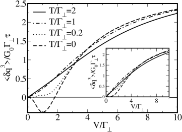
Figure 1: The voltage dependence of the third cumulant for different temperatures and zero magnetic field ($\Delta=0$) for $\Gamma_{-}/\Gamma_{\perp}=0$ (main graph), and for $\Gamma_{-}/\Gamma_{\perp}=0.9$ (inset).

We now briefly turn to the $g=1/2$ RT set–up. This set–up has caused much interest recently, see Ref. Komnik and Gogolin (2003a) and references therein. The Hamiltonian now is

$$H=H_{0}+\gamma(\psi_{L}d^{\dagger}+d\psi_{R}^{\dagger}+{\rm H.c})+\Delta d^{\dagger}d+H_{C}\;,$$ (13)

where $H_{0}$ stands for two biased LLs at $g=1/2$, $d$ is the electron operator on the dot, $\gamma$ is the tunneling amplitude and $H_{C}$ is an electrostatic interaction we do not write explicitly here (see Komnik and Gogolin (2003a)). Introducing $\lambda$ as standard, and carrying out the bosonization–refermionisation analysis, we find the same set of equations as for the Kondo dot, Eq. (5) and Eq.(6), but with $\lambda\to\lambda/2$ and $J_{\perp}=2\gamma$, $J_{\pm}=0$, when the Kondo statistics simplifies to binomial (unphysical case). Consequently, the FCS is given by a modification of the Levitov–Lesovik formula:

$$\chi_{1/2}(\lambda)=\chi_{0}^{1/2}(\lambda;2V;\{T_{\Delta}(\omega)\})\;,$$ (14)

with the effective transmission coefficient $T_{\Delta}(\omega)=4\gamma^{4}\omega^{2}/[4\gamma^{4}\omega^{2}+(\omega^{2}-\Delta^{2})^{2}]$ of the RT set-up in the symmetric case Komnik and Gogolin (2003a) (the contact asymmetry is unimportant). All the cumulants are thus obtainable from those of the non-interacting statistics Eq. (Full counting statistics for the Kondo dot.).

The $\Delta=0$ RT set–up is equivalent to the model of direct tunneling between two $g=2$ LLs Komnik and Gogolin (2003b). The latter model is connected by the strong to weak coupling ($1/g\to g$) duality argument to the $g=1/2$ Kane and Fisher model Kane and Fisher (1992), which is, in turn, equivalent to the CB set–up studied by KT. Therefore their FCS must be related to our Eq. (14) at $\Delta=0$ by means of the transformation: $T_{0}\to 1-T_{0}$ and $V\to V/2$. Indeed after some algebraic manipulation with KT’s Eq. (12), we find that the FCS for the CB set–up can be re–written as:

$$\chi_{CB}(\lambda)=\chi_{0}^{1/2}(-\lambda;V;\{1-T_{0}(\omega)\})\;.$$

To summarise, we derived the generating function for the charge transfer statistics for the Kondo dot in the Toulouse limit and analysed the third cumulant in detail. At low temperatures the transport is accomplished by electrons as well as electron pairs in the generic case whereas at $T=0$ the conventional binomial statistics is restored.

We wish to thank H. Grabert, R. Egger, B. Trauzettel, M. Kindermann and W. Belzig for inspiring discussions. This work was supported by the Landesstiftung Baden-Württemberg (Germany) and by the EU RTN DIENOW.

References

- Schottky (1918) W. Schottky, Ann. Phys. (Leipzig) 57, 541 (1918).
- Muzykantskii and Khmelnitskii (1994) B. A. Muzykantskii and D. E. Khmelnitskii, Phys. Rev. B 50, 3982 (1994).
- Cuevas and Belzig (2003) J. C. Cuevas and W. Belzig, Phys. Rev. Lett. 91, 187001 (2003).
- Jehl et al. (2000) X. Jehl, M. Sanquer, R. Calemczuk, and D. Mailly, Nature 405, 50 (2000).
- Levitov and Reznikov (2004) L. S. Levitov and M. Reznikov, Phys. Rev. B 70, 115305 (2004).
- Reulet et al. (2003) B. Reulet, J. Senzier, and D. E. Prober, Phys. Rev. Lett. 91, 196601 (2003).
- Levitov and Lesovik (1993) L. S. Levitov and G. B. Lesovik, JETP Lett. 58, 230 (1993).
- Bagrets and Nazarov (2003) D. A. Bagrets and Y. V. Nazarov, Phys. Rev. B 67, 085316 (2003).
- Kindermann and Nazarov (2003) M. Kindermann and Y. V. Nazarov, Phys. Rev. Lett. 91, 136802 (2003).
- Levitov (2003) L. S. Levitov, in Quantum Noise in Mesoscopic Systems, edited by Y. V. Nazarov (Kluwer, Dordrecht, 2003).
- Saleur and Weiss (2001) H. Saleur and U. Weiss, Phys. Rev. B 63, 201302 (2001).
- Safi and Saleur (2004) I. Safi and H. Saleur, Phys. Rev. Lett. 93, 126602 (2004).
- Andreev and Mishchenko (2001) A. V. Andreev and E. G. Mishchenko, Phys. Rev. B 64, 233316 (2001).
- Kindermann and Trauzettel (2004) M. Kindermann and B. Trauzettel, cond-mat/0408666 (2004).
- Matveev (1995) K. A. Matveev, Phys. Rev. B 51, 1743 (1995).
- Furusaki and Matveev (1995) A. Furusaki and K. A. Matveev, Phys. Rev. Lett. 75, 709 (1995).
- Feynman (1939) R. P. Feynman, Phys. Rev. 56, 340 (1939).
- Komnik and Gogolin (2005) A. Komnik and A. O. Gogolin, [in preparation] (2005).
- Emery and Kivelson (1992) V. J. Emery and S. Kivelson, Phys. Rev. B 46, 10812 (1992).
- Gogolin et al. (1998) A. O. Gogolin, A. A. Nersesyan, and A. M. Tsvelik, Bosonization and Strongly Correlated Systems (Cambridge University Press, 1998).
- Schiller and Hershfield (1998) A. Schiller and S. Hershfield, Phys. Rev. B 58, 14978 (1998).
- Komnik and Gogolin (2003a) A. Komnik and A. O. Gogolin, Phys. Rev. Lett. 90, 246403 (2003a).
- Komnik and Gogolin (2003b) A. Komnik and A. O. Gogolin, Phys. Rev. B 68, 235323 (2003b).
- Kane and Fisher (1992) C. L. Kane and M. P. A. Fisher, Phys. Rev. B 46, 15233 (1992).