Explaining the Magnetic Moment Reduction of Fullerene encapsulated Gadolinium through a Theoretical Model

Abstract

We propose a Theoretical model accounting for the recently observed reduced magnetic moment of Gadolinium in fullerenes. While this reduction has been observed also for other trivalent rare-hearth atoms (Dy³⁺, Er³⁺, Ho³⁺) in fullerenes and can be ascribed to crystal field effects, the explanation of this phenomena for Gd³⁺ is not straightforward due to the sphericity of its ground state ( S$=7/2$ , L$=0$ ). In our model the momentum lowering is the result of a subtle interplay between hybridisation and spin-orbit interaction.

I INTRODUCTION

Endohedral metallofullerenes M@$C_{82}$ are novel materials that have attracted a wide interest in physics, chemistry but also in material or biological sciences for the large variety of promising applications of their peculiar propertiesshi1 ; bet1 ; she1 . In endohedral metallofullerenes, a positively charged core metal is off-center in a negatively charged strong carbon cage, resulting in strong metal-cage interaction and intrafullerene charge transfer from the metal to the cage.shi1 ; poi1 ; gie1 ; iid1

The magnetism of these systems is mainly due to the spin of the entrapped metals. In a series of average magnetization mesurements a paramagnetic behaviour has been observed fun1 ; nut1 ; dun1 ; hua1 , with negative Weiss temperatures. The negative Weiss temperature indicates the presence of a weak antiferromagnetic interaction betwen the cage and the metal, and between neighbooring cages, but for heavy rare-earths (RE) endofullereneshua1 ferromagnetic coupling has been mentioned in the sub-20K range. In the case of heavy RE these experiments gave a number of magnetons per encaged ion that is smaller than for the free ion. This result has been phenomenogically ascribed to the cage crystal field interaction for high L ions and, for the $L=0$ Gd case, to the antiferommagnetic interaction between the ion and the cage.

A recent workdenadai has used x-ray magnetic circular dichroism and (XMCD) x-ray absorption spectroscopy (XAS) to characterize local magnetic properties of heavy RE metallo centers, using the $M_{4}$ and $M_{5}$ resonances ($3d\rightarrow 4f$ transitions). The absorption spectra of this work were very well fitted assuming trivalent ions ($4f^{n}$ electronic structure with $n=7$ for Gd, $n=9$ for Dy…), while XMCD confirmed that there is a strong reduction of the measured ion magnetisation compared to the free ion case.

For $L\neq 0$ ions the reduction was reproduced by a model Hamiltonian were a weak crystal field prevents the ion total angular moment $J$ to align completely along the magnetic field. The case $L=0$ of trivalent Gadolinium was more difficult and hybridisation model gave not a satisfactory explanation.

Infact, althought hybridisation gives antiferromagnetic coupling with the cage and accounts ( in the Gd case) for a 14% reduction of the average moment ( Gd + cages), it cannot explain the reduction of the moment localized on Gd ion (see next section).

What we will show in the present paper is that a combined action of hybridisation and spin-orbit interaction can have a dramatic effect on the observed magnetic moment.

This effect is not trivial and is significant only in a restraint parameters region that was not discovered in the previous numerical studydenadai . In the present paper we will give a complete analytical discussion of this effect. In next section we will introduce a simple model with an anisotropic hybridisation where the Gd ground state is basically $4f^{7}$ with a small $4f^{8}$ component due to a backdonation from the cage. we will then consider spin-orbit interactions at the first order and show the dramatic changes in magnetisation. Analytical formula will be compared to exact numerical solutions. Finally we will discuss the possible experimental manifestations of the studied phenomena.

II Hybridisation Model and spin-orbit

Back donation concerns a cage unpaired electron. As the Re ion is off center we consider that the hopping is non isotropic and choose to restrain the transfer of the cage backdonated electron to the $4f$ orbital that is closest to the cage, the $m_{z}=0$ one, where the z-axis is parallel to the off center displacement.

The Gd ground state has $S=7/2$, $L=0$. Adding one more electron to this state, one can acces only the quantum numbers $S=3$, $L=3$ of the $4f^{8}$ configurationrachaIII .

The energy difference between the $4f^{8}$ level and $4f^{7}$ ground state will be named, without SO coupling, $\Delta E$. This is a positive scalar quantity and must be large in magnitude, compared to the hopping strenght $t$, because the fractional backdonation has been observed to be very small.

We consider an effective interaction term proportional to $t^{2}$. This interaction transforms the state ($S_{z},s$) (where $S_{z}$ is the spin z-component of the $4f^{7}$ shell and s the cage unpaired electron one) into the state ($S_{z}+2s,-s$), and the other way round.

We can therefore restrict the effective Hamiltonian to the two-dimensional space spanned by ($S_{z},s$) and ($S_{z}+2s,-s$ ). The elements of the effective interactions are :

$$H(S_{z},s\rightarrow S_{z}+s-s^{{}^{\prime}},s^{{}^{\prime}})=$$ (1)

$$-t^{2}\sum_{\eta}\frac{\langle S_{z}+s-s^{{}^{\prime}}|c_{0s^{{}^{\prime}}}|\eta\rangle\langle\eta|c^{+}_{0s}|S_{z}\rangle}{E_{\eta}-E_{0}}$$

where $E_{0}$ is the $4f^{7}$ ground state energy, $c^{+}_{ms}$ and $c_{ms}$ are creation/annihilation operators for a $4f$ electrons with $m_{z}=m$ and $s_{z}=s$. The sum runs over the states $\eta$ of the $4f^{8}$ configuration.

The case of Gd is quite simple because the only $4f^{8}$ state having a non-zero parentage coefficient with $|4f^{7}S=7/2L=0\rangle$ ground state is $|4f^{8}S^{{}^{\prime}}=3,L^{{}^{\prime}}=3\rangle$.

The results of operating on the ground state on $4f^{7}$ can be expressed in terms of the parentage coefficients and angular recoupling factors using well known formulasureau , for our specific case:

$$c^{+}_{0s}|4f^{7}SS_{z}M_{z}\rangle=-\sqrt{8}G^{S^{{}^{\prime}}L^{{}^{\prime}}}_{SL}\times$$

$$(SS_{z}1/2s;S^{{}^{\prime}}(S_{z}+s))\times|4f^{8}SL(S_{z}+s)M_{z}\rangle$$ (2)

Putting this formula into (1) the Hamiltonian can be written as :

$$H=-\frac{t^{2}}{\Delta E}\frac{8}{7}v_{S_{z}}\otimes v_{S_{z}}$$ (3)

where $v_{S_{z}}$ is the versor :

$$v_{S_{z}}=((7/2+S_{z})^{1/2},-(7/2-S_{z}+1)^{1/2})\frac{1}{\sqrt{8}}$$ (4)

For positive $\Delta E$ the ground state of H is $v_{S_{z}}$, it corresponds to antiferromagnetic alinement ( total angular moment $J=3$), and has energy $-\frac{t^{2}}{\Delta E}\frac{8}{7}$.

The state perpendicular to $v_{S_{z}}$ has energy zero and corresponding total angular moment $J=4$. There is no energy dependency on $S_{z}$ as it could have been expected on the basis of rotational invariance in the spin space, as long as spin-orbit interaction is not included. The local moment of Gd, in the antiferromagnetic ground state, can be almost fully aligned along the magnetic field. On the basis of equation (4) one should observe, at saturation

$$\langle S_{z}\rangle=(7/2\times 7+5/2)/8=3.375$$ (5)

corresponding to a $3.6$% reduction which is very far from the $20$% observed one. The antiferromagnetic metal-cage coupling cannot explain the moment reduction observed with XAS, XMCD techniques.

Therefore we add the spin-orbit (SO) coupling to the picture which breaks rotational invariance in the spin space. At first order SO splits the energies of the $S^{{}^{\prime}}=3$ $L^{{}^{\prime}}=3$ state according to the total $J^{{}^{\prime}}$, and affects the denominator involved in equation (1). As a result the equation for H, that is given by equation 3 for the zero-SO case, must be rewritten in this form :

$$H_{SO}(S_{z})=F(S_{z})v_{S_{z}}\otimes v_{S_{z}}$$ (6)

where

$$F(S_{z})=-t^{2}\frac{8}{7}\sum_{J^{{}^{\prime}}}\frac{(2J^{{}^{\prime}}+1)(\begin{array}[]{ccc}3&3&J^{{}^{\prime}}\\ S_{z}^{{}^{\prime}}&0&-S_{z}^{{}^{\prime}}\end{array})^{2}}{\Delta E+E^{SO}_{J^{{}^{\prime}}}}$$ (7)

where $S_{z}^{{}^{\prime}}=S_{z}-1/2$. From a formal point of view SO gives at first order also another contribution beside affecting the propagator denominator. In fact the $4f^{7}$ ground state, considering SO interaction, is not a pure $S=7/2$ , $L=0$ state, but it has also a small component of the state $S=5/2$, $L=1$, whose amplitude is first order in SO strength. It is this perturbed ground state that should be considered in equation (1). However for symmetry reasons, in the framework of our model where backdonation affects only the $m_{z}=0$ orbital, the contribution at first order in SO coming from this $S=5/2$, $L=1$ component is zero.

At the moment we will therefore restrain the discussion to the above equation (7), that contains all the important physics of the studied phenomena.

The $S_{z}$ dependency in equation (7) is given by the $J^{{}^{\prime}}$ dependecy of $E^{SO}_{J^{{}^{\prime}}}$. If the denominator in equation (7) is constant, one can factor the term :

$$\sum_{J^{{}^{\prime}}}(2J^{{}^{\prime}}+1)(\begin{array}[]{ccc}3&3&J^{{}^{\prime}}\\ S_{z}^{{}^{\prime}}&0&-S_{z}^{{}^{\prime}}\end{array})^{2}=1$$ (8)

and obtain again equation (3). For the $4f^{8},S^{{}^{\prime}}=3,L^{{}^{\prime}}=3$ state the energy $E^{SO}_{J^{{}^{\prime}}}$ is

$$E^{SO}_{J^{{}^{\prime}}}=\zeta_{nl}\frac{24-J^{{}^{\prime}}(J^{{}^{\prime}}+1)}{12}$$ (9)

where $\zeta_{nl}$ is the strength of SO interaction. This equation can be obtained in a simple way : the state obtained putting seven spin-up electrons in the 4f shell, plus one spin-down electron in the $m_{z}=3$ state, has $S=3$, $L=3$, $J=6$.

It is very easy to calculate for this mono-determinantal state the expectation value of the $S.L$ scalar operator, it is $-1.5$ ( $m_{z}=3$ of the eighth electron times its spin ). The expectation values for the other $J^{{}^{\prime}}$ can be calculated observing that the expectation value of a scalar product of two $L=1$ tensors must be proportional to the 6J factor for the angular moments sextet (3,3,$J^{{}^{\prime}}$,1,1,0). By a quick glance at sixJ tables, equation (9) is readily obtained.

The energy correction $E^{SO}_{J^{{}^{\prime}}}$, considering $\zeta_{nl}=0.1975eV$thole has the negative value of about $-0.3$eV for $J^{{}^{\prime}}=6$ and a positive value of about $0.4$eV for $J^{{}^{\prime}}=0$. These values have to be compared to $\Delta E$. Taking $\Delta E$ of the order of $1eV$ the effect of $E^{SO}_{J^{{}^{\prime}}}$ is not negligeable and the dependency on $S_{z}$ is given mainly by the term with the smaller denominator, the $J^{{}^{\prime}}=6$ term. The Wigner symbol

$$(\begin{array}[]{ccc}3&3&6\\ S_{z}^{{}^{\prime}}&0&-S_{z}^{{}^{\prime}}\end{array})$$ (10)

has the bigger value for the smaller $S_{z}^{{}^{\prime}}$, as one can understand classically considering that to get $J^{{}^{\prime}}=6$ one has to align $S^{{}^{\prime}}$ and $L^{{}^{\prime}}$.

Therefore the ground state has the smallest $S^{{}^{\prime}}_{z}$ and, unless the polarising magnetic field is sufficiently strong, the observed local magnetic moment will be zero.

The $J^{{}^{\prime}}=6$ term is the only one to consider for $\Delta E$ approaching the value of $0.3$ eV, because its denominator in equation (7) tends to zero. But a small denominator means strong hybridisation, while hybridisation is weak because the encaged Gd is an almost pure $4f^{7}$ configuration.

One should therefore consider the region where $\Delta E+E^{SO}_{J^{`}}$ is big compared to the hopping strenght. For $\Delta E$ going to infinity the studied effect cancels out( see equation (8)).

So we are going to study a region where the effect results from a imperfect cancellation of the different terms involved in the sum of equation (7).

As a cancellation is involved one has to be very precise evaluating each single term in the sum. Therefore we devote a particular attention to the exact values of $E^{SO}_{J^{{}^{\prime}}}$.

These values could be obtained at second order using Racah formalism and summing contributions from all the $4f^{8}$ states accessible operating with the spin-orbit interaction on the $4f^{8},S=3,L=3$ state. However, for the scope of this paper, which is to clarify the consequences of equation (7), it is sufficient to plug in the sum the energies obtained by exact diagonalisation of $Gd^{2+}$ ion.

We show in table (1) the comparison of $E^{SO}_{J^{{}^{\prime}}}$ energies, calculated at first order by equation (9), compared with the exact numerical result.

The numerical value of $E^{SO}_{J^{{}^{\prime}}}$ is obtained calulating numerically the energy eigenvalues of the $4f^{8}$ Hamiltonian, and subtracting the ground state energy of the $4f^{7}$ one, where SO interaction is accounted for in both Hamiltonians. In the numerical calculation $F_{2},F_{4},F_{6}$ are taken from Tholethole . The parameter $F_{0}$ is already contained in $\Delta E$, so we take $F_{0}$ equal to zero in numerical calculations.

In figure (1) we show the energies as a function of $\Delta E$ for the antiferromagnetic eigenstates of $H^{SO}(S_{z})$ ( equation (6) ) for $S^{{}^{\prime}}_{z}$ between $1$ (smallest energy ) and $3$ (highest energy), with a dashed line, compared to the exact numerical solution ( solid line). The ground state energy for $S^{{}^{\prime}}_{z}=0$ has been subtracted (it is taken as origin of the energy scale). In the left panel the $4f^{8}$ energies entering equation(6) are calculated at first first order in SO, while in the right panel numerical $4f^{8}$ energies for an isolated ion are used. The parameters used in the calculation are $t=0.05eV$ and $\Delta E$ between $0.4$ and $1$. One can observe that the simple formula 6 is an excellent approximation when exact energies are considered in the denominator.

The energy splitting has to be compared with the magnetic field strength. Considering a typical XAS-XMCD experimental case denadai with a $7$ Tesla field, the energy gain got aligning about $7$ Bohr magnetons from perpendicular to parallel direction with the field is 0.4meV. This energy is of the same order of magnitude of, or lower, than the splitting caused by hybridisation plus spin-orbit.

This effect can therefore, depending on $t$ and $\Delta E$, prevail on the magnetic polarizing field and suppress partially, or completely, the magnetization.

	$j=6$	$j=5$	…	..	..	..	$j=0$
eq. 9	-0.295	-0.098	0.065	0.197	0.295	0.361	0.394
$E_{4f^{8}}-E_{4f^{7}}$	-0.302	-0.066	0.076	0.189	0.268	0.321	0.346

Table 1: Dependancy of $4f^{8}$ ground states as a function of total moment J. First order formula ( first line) is compared to numerical results ( second line ) obtained using parameters from reference thole . Units are eV.

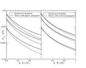
Figure 1: Energies as a function of $\Delta E$ for $S^{{}^{\prime}}_{z}$ between $1$ (smallest energy ) and $3$ (highest energy). The ground state for $S^{{}^{\prime}}_{z}=0$ is taken as origin of the energy scale. The dashed line is equation (6) with $4f^{8}$ energies energies at first order in SO (left) and calculated numerically for an isolated ion (right). Comparison is made with the exact numerical solution ( solid line).

III Discussion and Conclusions

We have shown in the previous section that a very small anisothropic hybridisation ( $t=0.05$ eV ) can give, for weak magnetic fields, a complete suppression of the magnetisation along the encaged metal displacement axis. At zero temperature the magnetization would be a discontinuous function of the magnetizing field. For a polarizing field perpendicular to the displacement axis the magnetization curve would be instead continuous.

In a real system one should take into account temperature and disorder. Temperature effect would tend to smear discontinuities.

Disorder may be of different kinds. One kind of disorder are fluctuations in $\Delta E$ due to inhomogeneities of cage environments. As $\Delta E$ affects the propagator denominator of equation (7) fluctuations might influence greatly the experimental result: discontinuities could be smeared out because the moment of cages having lower $\Delta E$ is depressed more than that of higher $\Delta E$ ones.

Disorder of the displacement axis direction in the sample would have a similar effect.

These consideration could explain why experiments show magnetization curves that are continuous and saturate at reduced values.

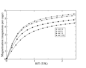
Figure 2: Magnetisation $1.8$,$3$,$6$ and $8$K temperature for the parameters choice $\Delta E=1eV$ and $t=0.2eV$.

As an example we calculate magnetisation curves at different temperature in the case of random orientation of the displacement axis. We consider the parameters $\Delta E=1eV$ and $t=0.2eV$. The magnetisation is shown in figure 2 for $1.8$,$3$,$6$ and $8$K. These data have to be compared with figure 8 of referencehua1 . The experimental behaviour is reproduced.

The above discussion leaves the problem still open. First of all further investigation is needed to better evaluate the real values of $\Delta E$ and $t$, that in this work we have chosen arbitrarily with the only criteria of giving a numerical example based on conservative values ( small $t$ and non negligeable $\Delta E$).

Second, a comparison with a complete set of data using a realistic modelisation of the sample should be done.

However we can conclude that the effect is important even for very small hybridization, and therefore cannot be ignored if one wants really to understand the magnetic properties of encaged RE.

- (1) H. Shinohara, Rep. Prog. Phys. 63, 843 (2000).
- (2) D.S. Bethune, R. D. Johnson, J. R. Salem, M. S. deVries and C. S. Yannoni, Nature 366, 123 (1993).
- (3) B. S. Sherigara, W. Kutner and F. D’Souza, Electroanalysis, 15, 753 (2003).
- (4) D. M. Poirier, M. Knupfer, J. H. Weaver, W. Andreoni, K. Laasonen, M. Parrinello, D. S. Bethune, K. Kikuchi and Y. Achiba, Phys. Rev. B 49, 17403 (1994)
- (5) H. Giefers, F. Nessel, S. I. Gy ry, M. Strecker, G. Wortmann, Y. S. Grushko, E. G. Alekseev and V. S. Kozlov, Carbon 37, 721 (1999)
- (6) S. Iida, Y. Kubozono, Y. Slovokhotov, Y. Takabayashi, T. Kanbara, T. Fukunaga, S. Fujiki, S. Emura and S. Kashino, Chem. Phys. Lett. 338, 21 (2001).
- (7) H. Funasaka, K. Sugiyama, K. Yamamoto and T. Takahashi, J. Phys. Chem. 99, 1826 (1995).
- (8) C. J. Nuttal, Y. Inada, Y. Watanabe, K. Nagai, T. Muro, D. H. Chi, T. Takenobu, Y. Iwasa and K. Kikuchi, Mol. Cryst and Liq. Cryst. 340, 635 (2000)
- (9) L. Dunsch, D. Eckert, J. Froehner, A. Bartl, P. Kuran, M. Wolf and K. H. Mueller, In Fullerenes: Recent Advances in the Chemistry and Physics of Fullerenes and Related Materials 1998, 6, 955, ed. K. Kadish and R. Ruoff (Pennington: Electrochemical Society).
- (10) H.J. Huang, S. H. Yang and X. X. Zhang, J. Phys. Chem. B 104, 1473 (2000)
- (11) C. De Nadaï, A. Mirone, S. S. Dhesi, P. Bencok, N. B. Brookes, I. Marenne, P. Rudolf, N. Tagmatarchis, H. Shinohara, and T. J. S. Dennis, Phys. Rev. B 69, 184421 (2004)
- (12) G. Racah Phys. Rev. 76, 1352-1365 (1949)
- (13) A. Sureau, International Journal of Quantum Chemistry, Vol. V, 599-603 (1971)
- (14) B. T. Thole, G. van der Laan, J. C. Fuggle, G. A. Sawatzky, R. C. Karnatak and J. -M. Esteva, Phys. Rev. B 32, 5107 (1985).