Superconductivity and Density Wave in the Quasi-One-Dimensional Systems: Renormalization Group Study

Abstract

The anisotropic superconductivity and the density wave have been investigated by applying the Kadanoff-Wilson renormalization group technique to the quasi-one-dimensional system with finite-range interactions. It is found that a temperature ($T$) dependence of response functions is proportional to $\exp(1/T)$ in a wide region of temperature even within the one-loop approximation. Transition temperatures are calculated to obtain the phase diagram of the quasi-one-dimensional system, which is compared with that of the pure-one-dimensional system. Next-nearest neighbor interactions ($V_{2}$) induce large charge fluctuations, which suppress the $d_{x^{2}-y^{2}}$-wave singlet superconducting ($d$SS) state and enhance the $f$-wave triplet superconducting ($f$TS) state. From this effect, the transition temperature of $f$TS becomes comparable to that of $d$SS for large $V_{2}$, so that field-induced $f$-wave triplet pairing could be possible. These features are discussed to comprehend the experiments on the (TMTSF)₂PF₆ salt.

1 Introduction

The mechanism of superconductivity in quasi-one-dimensional (q1d) systems has been attracting renewed interest since the appearance of the triplet superconductivity suggested in the experiments on the q1d organic conductor (TMTSF)₂PF₆. [1, 2] In the phase diagram of (TMTSF)₂PF₆[3], the superconducting phase is adjacent to the spin density wave (SDW) phase. From the knowledge of the anisotropic superconductivity,[4, 5, 6] which have been extensively enriched for two decades, the $d$-wave singlet superconductivity ($d$SS) is expected to occur in such superconducting phase. However, recent experiments on (TMTSF)₂PF₆ indicate a counter example of this widespread knowledge. The unsaturated magnitude of the upper critical field $H_{{\rm c}2}$[1] and the constant Knight shift thorough the superconducting transition temperature $T_{\rm c}$[2] strongly suggest the formation of triplet pairing. In addition, the SDW phase turned out to be an exotic one, in which the $2k_{F}$ charge density wave (CDW) coexists with the $2k_{F}$-SDW as seen from the X-ray experiments.[7, 8]

The theoretical study of q1d systems is complicated due to its dimensionality originated from the anisotropy, where the effects of the one-dimensional (1d) fluctuation are essential to understand its physics. In the system with the 1d fluctuation, there are equally divergent contributions from both Cooper (electron-electron) and Peierls (electron-hole) channels. However, the 1d fluctuation cannot be evaluated correctly by the conventional method such as the random phase approximation (RPA)[9], the fluctuation exchange (FLEX) approximation[10, 11] or the third-order perturbation theory,[12] which are powerful for the study of three- or two-dimensional anisotropic superconductivity. On the other hand, the renormalization group (RG) technique based on the g-ology is extremely useful for the treatment of the 1d fluctuation, whereas it is complicated to deal with anisotropic superconducting states, such as $d$SS.

Recently, Duprat and Bourbonnais extended the technique of Kadanoff-Wilson RG for purely 1d systems to that for q1d systems.[13] This technique enabled us to treat both 1d fluctuations and various kinds of anisotropic superconductivity. Meanwhile, the essential role of charge fluctuation has been pointed out phenomenologically.[11, 14] Quite recently, it is shown by the RPA[15] that charge fluctuations induced by next-nearest repulsive interactions can give rise to the $f$-wave triplet superconductivity ($f$TS), though the 1d fluctuation effects are still pushed aside.

The purpose of the present paper is to get a deep insight into the interplay of the superconductivity and the density waves in q1d systems in terms of the Kadanoff-Wilson RG technique developed for q1d system. Especially, we shall focus on clarifying i) crossover from purely 1d case into q1d case, ii) effects of long-range Coulomb interactions and iii) microscopic mechanism of the q1d superconductivity, considering the effect of the 1d fluctuation.

In §2, we briefly describe the Kadanoff-Wilson RG technique. Next, the method of the present work. In §3, it is shown that the response functions exhibit a noticeable property being proportional to $\exp(1/T)$. Phase diagrams for several magnitudes of interchain hopping are demonstrated on the plane of intrachain interactions. Transition temperatures as a function of the interchain hopping, are also presented. Then a discussion of the mechanism of the q1d superconductivity is given. Section 4 is devoted to conclusion and a comparison of the present result and the experiments.

2 Formulation

2.1 Model

We consider a system consisting of an array of $N_{b}$ chains of length $L$, which is described by the Hamiltonian,

$$H =\sum_{p,{\bf k},\sigma}\xi({\bf k})a^{\dagger}_{p{\bf k}\sigma}a_{p{\bf k}\sigma}$$

$$+\frac{\pi v_{F}}{LN_{b}}\sum_{{\bf k}_{i},{\bf q},\sigma}(g_{2}\delta_{\sigma_{1}\sigma_{4}}\delta_{\sigma_{2}\sigma_{3}}-g_{1}\delta_{\sigma_{1}\sigma_{3}}\delta_{\sigma_{2}\sigma_{4}})$$

$$\times a_{+,{\bf k}_{1}+{\bf q}\sigma_{1}}^{\dagger}a_{-,{\bf k}_{2}-{\bf q}\sigma_{2}}^{\dagger}a_{-,{\bf k}_{2}\sigma_{3}}a_{+,{\bf k}_{1}\sigma_{4}}.$$ (1)

The first term denotes the band energy with the q1d dispersion:

$$\xi({\bf k}) =-2t_{a}\cos k_{a}-2t_{b}\cos k_{b}-\mu$$

$$\simeq v_{F}(|k_{a}|-k_{F}^{0})-2t_{b}\cos k_{b}+2t_{b}^{\prime}\cos 2k_{b},$$ (2)

where the intrachain electron spectrum with the nearest intrachain hopping $t_{a}$ is linearized at the Fermi points $\pm k_{F}^{0}$ with the Fermi velocity $v_{F}$, and $\mu$ is the chemical potential. In Eq. (1), $a_{p{\bf k}\sigma}^{\dagger}$ ($a_{p{\bf k}\sigma}$) is a creation (an annihilation) operator close to the right $k_{a}=+k_{F}^{0}$ $(p=+)$ and the left $k_{a}=-k_{F}^{0}$ $(p=-)$ Fermi surface, respectively. The second and third terms of Eq. (2) denote the nearest interchain hopping $t_{b}$ and the next-nearest interchain hopping $t_{b}^{\prime}$, respectively, where

$$t_{b}^{\prime}=\frac{t_{b}^{2}\cos(k_{F}^{0})}{4t_{a}\sin^{2}(k_{F}^{0})},$$ (3)

is obtained as the nesting deviation. For the interaction part, the second term of Eq. (1), we follow the standard notations of the g-ology, where $g_{1}$ corresponds to backward scattering and $g_{2}$ does to forward scattering. (Note that $g_{1,2}$ are normalized by $\pi v_{F}$ here.) For the 1/4-filling case, $g_{1}$ and $g_{2}$ are given in terms of on-site $U$, nearest-neighbor $V_{1}$ and next-nearest-neighbor $V_{2}$ interactions, as

$$\pi v_{F}g_{1} =U/2-V_{2},$$ (4)

$$\pi v_{F}g_{2} =U/2+V_{1}+V_{2}.$$ (5)

In order to examine superconductivity and density wave in terms of RG technique, we utilize the path integral method[13], where the partition function $Z$ ($={\rm Tr}e^{-\beta H}$) is given by

$$Z=\int\!\!\!\int\mathcal{D}\psi^{*}\mathcal{D}\psi\exp(S[\psi^{*},\psi]_{\ell}),$$ (6)

and the effective action $S$ is written in the form,

$$S[\psi^{*},\psi]_{\ell} =S_{0}[\psi^{*},\psi]_{\ell}+S_{\rm I}[\psi^{*},\psi]_{\ell},$$ (7)

$$S_{0}[\psi^{*},\psi]_{\ell} =\sum_{p,\sigma,\{\tilde{{\bf k}}\}^{*}}[G_{p}^{0}(\tilde{{\bf k}})]^{-1}\psi_{p,\sigma}^{*}(\tilde{{\bf k}})\psi_{p,\sigma}(\tilde{{\bf k}}),$$ (8)

$$S_{\rm I}[\psi^{*},\psi]_{\ell} =-\pi v_{F}\sum_{\mu,\tilde{\bf Q}}J_{\mu}(k_{1b},k_{2b},q_{b};\ell)O_{\mu}^{{\rm P}*}(\tilde{\bf Q})O_{\mu}^{\rm P}(\tilde{\bf Q}),$$ (9)

$$=-\pi v_{F}\sum_{\mu,\tilde{\bf q}}W_{\mu}(k_{1b},k_{2b},q_{b};\ell)O_{\bar{\mu}}^{{\rm C}*}(\tilde{\bf q})O_{\bar{\mu}}^{\rm C}(\tilde{\bf q}),$$ (10)

where the renormalization of the bandwidth is defined as

$$E_{0}(\ell)=E_{0}\exp(-\ell),$$ (11)

with the bandwidth cut-off $E_{0}$. The quantities $\psi(\tilde{\bf k})$ and $\psi^{*}(\tilde{\bf k})$ are the Grassmann fields and $\tilde{\bf k}=({\bf k},\omega_{n})$. $\{{\bf k}\}^{*}$ denotes the renormalized momentum space. The operator $O_{\mu}^{{\rm P}}$ denotes Peierls fields

$$O_{\mu}^{{\rm P}}(\tilde{\bf Q})=\sqrt{\frac{T}{LN_{b}}}\sum_{\alpha,\beta,\{\tilde{\bf k}\}^{*}}\psi_{-,\alpha}^{*}(\tilde{\bf k}-\tilde{\bf Q})\sigma_{\mu}^{\alpha\beta}\psi_{+,\beta}(\tilde{\bf k}),$$ (12)

describing the CDW ($\mu=0$) and the SDW ($\mu=1,2,3$) channels, where $\tilde{\bf Q}=(2k_{F}^{0}+Q_{0},Q_{b},\omega_{m}=0,\pm 2\pi T,\cdots)$ ($Q_{0}\ll 2k_{F}^{0}$). The operator $O_{\bar{\mu}}^{{\rm C}}$ is Cooper fields

$$O_{\mu}^{{\rm C}}(\tilde{\bf q})=\sqrt{\frac{T}{LN_{b}}}\sum_{\alpha,\beta,\{\tilde{\bf k}\}^{*}}\alpha\psi_{-,-\alpha}^{*}(-\tilde{\bf k}+\tilde{\bf q})\sigma_{\bar{\mu}}^{\alpha\beta}\psi_{+,\beta}(\tilde{\bf k}),$$ (13)

for singlet ($\bar{\mu}=0$) and triplet ($\bar{\mu}=1,2,3$) pairing, where $\tilde{\bf q}=(q_{0},q_{b},\omega_{m})$ ($q_{0}\ll 2k_{F}^{0}$). The couplings $J_{\mu}$ and $W_{\bar{\mu}}$ correspond to that of the density wave and the superconductivity respectively, and are related to $g_{1,2}$ as $J_{\mu=0}=g_{1}-g_{2}/2$, $J_{\mu\neq 0}=-g_{2}/2$, $W_{\bar{\mu}=0}=-(g_{1}+g_{2})/2$ and $W_{\bar{\mu}\neq 0}=(g_{1}-g_{2})/2$, respectively.

2.2 Renormalization of couplings $J_{\mu}(\ell)$, $W_{\bar{\mu}}(\ell)$

First we apply the RG technique to coupling constants for the Peierls and the Cooper channel. By taking contraction of each channel, the one-loop flow equation are obtained as[13]

$$\frac{d}{d\ell}J_{\mu} (Q_{b}-k_{b},k_{b};\ell)$$

$$=\frac{1}{N_{b}}\sum_{\bar{\mu},k_{b}^{\prime}}c_{\mu,\bar{\mu}}W_{\bar{\mu}}(Q_{b}-k_{b},k_{b}^{\prime};\ell)W_{\bar{\mu}}(k_{b}^{\prime},k_{b};\ell)I_{\rm C}(\ell)$$

$$-J_{\mu}(Q_{b}-k_{b},k_{b};\ell)\frac{1}{N_{b}}\sum_{k_{b}^{\prime}}J_{\mu}(Q_{b}-k_{b}^{\prime},k_{b}^{\prime};\ell)I_{\rm P}(Q_{b},k_{b}^{\prime};\ell),$$ (14)

where $c_{0,0}=-1/2,c_{0,\bar{\mu}\neq 0}=1/2,c_{\mu\neq 0,0}=1/2$ and $c_{\mu\neq 0,\bar{\mu}\neq 0}=1/6$. The first term of the right-hand side of Eq. (14) corresponds to the contraction in the Cooper channel, where $I_{\rm C}(\ell)d\ell=\tanh[E_{0}(\ell)/4T]d\ell$ is the outer-shell integration. The second term corresponds to the contraction in the Peierls channel, with the outer-shell integration

$$I_{\rm P}(Q_{b},k_{b1},\ell)d\ell =\frac{E_{0}(\ell)d\ell}{4}\sum_{\lambda=\pm 1}\frac{1}{E_{0}(\ell)+\lambda A(k_{b1},Q_{b})}$$

$$\times\biggl{[}\tanh\frac{E_{0}(\ell)}{4T}+\tanh\frac{1}{2T}\bigl{\{}\frac{E_{0}(\ell)}{2}+\lambda A(k_{b1},Q_{b})\bigr{\}}\biggr{]},$$ (15)

$$A(k_{b},Q_{b}) =2t_{b}[\cos k_{b}+\cos(k_{b}+Q_{b})]$$

$$+2t_{b}^{\prime}[\cos 2k_{b}+\cos 2(k_{b}+Q_{b})].$$ (16)

For $t_{b}=0$, the flow equation (14) yields the one-loop 1d flow equations.[16, 17] Note that $I_{\rm C}(\ell)$ is a constant while $I_{\rm P}(Q_{b},k_{b},\ell)$ suppressed by $t_{b}^{\prime}$ depending on the wave vector of particles. Thus the Cooper channel is always singular (i.e., does not depend on the shape of the Fermi surface) while the Peierls channel is suppressed by the nesting deviation. The renormalized Cooper couplings are obtained from the renormalized Peierls couplings through the relation

$$W_{\bar{\mu}=0}(Q_{b}-k_{b},k_{b};\ell) =-\frac{1}{2}J_{0}(Q_{b}-k_{b},k_{b};\ell)$$

$$\hskip 14.22636pt+\frac{3}{2}J_{\mu\neq 0}(Q_{b}-k_{b},k_{b};\ell),$$ (17)

$$W_{\bar{\mu}\neq 0}(Q_{b}-k_{b},k_{b};\ell) =\frac{1}{2}J_{0}(Q_{b}-k_{b},k_{b};\ell)$$

$$\hskip 14.22636pt+\frac{1}{2}J_{\mu\neq 0}(Q_{b}-k_{b},k_{b};\ell),$$ (18)

which is obtained from Eqs. (9) and (10) straightforwardly.

Following the idea of the dimensional crossover theory[16, 18], we adopt two-step RG procedure. First we apply the RG technique of 1d[16] (1d RG) to the regime above the crossover temperature $T_{\rm cross}$, and then that of q1d[13] (q1d RG) to the region below $T_{\rm cross}$ as the second step. For the first step, we adopt the two-loop flow equations of 1d[16]

$$\frac{dg_{1}(\ell)}{d\ell} =-g_{1}(\ell)^{2}-\frac{1}{2}g_{1}(\ell)^{3},$$ (19)

$$\frac{dG(\ell)}{d\ell} =0,$$ (20)

where $G(\ell)\equiv g_{1}(\ell)-2g_{2}(\ell)$. During the 1d RG, the interchain coupling $j_{\mu}$ due to the pair hopping is produced as follows:

$$j_{\mu}(\ell) =z(\ell)^{-2}f_{\mu}(\ell),$$ (21)

$$\frac{df_{\mu=0}(\ell)}{d\ell} =\biggl{[}\frac{(g_{2}(\ell)-2g_{1}(\ell))z(\ell)t_{b}}{E_{0}(\ell)}\biggr{]}^{2},$$ (22)

$$\frac{df_{\mu\neq 0}(\ell)}{d\ell} =\biggl{[}\frac{g_{2}(\ell)z(\ell)t_{b}}{E_{0}(\ell)}\biggr{]}^{2},$$ (23)

where flow equations for $t_{b}$ and $z$ (corresponding to self energy) are

$$\frac{d}{d\ell}\ln t_{b}(\ell) =1-\frac{1}{4}\bigl{[}g_{1}(\ell)^{2}+g_{2}(\ell)^{2}-g_{1}(\ell)g_{2}(\ell)\bigr{]},$$ (24)

$$\frac{d}{d\ell}\ln z(\ell) =-\frac{1}{4}\bigl{[}g_{1}(\ell)^{2}+g_{2}(\ell)^{2}-g_{1}(\ell)g_{2}(\ell)\bigr{]},$$ (25)

respectively. The dimensional crossover temperature is given by $T_{\rm cross}=E_{0}(\ell_{\rm cross})/2$, where $\ell_{\rm cross}$ is defined as $E_{0}(\ell_{\rm cross})=t_{b}(\ell_{\rm cross})$. Thus the initial couplings for the second step, i.e., q1d RG, are given by a combination of $g_{\mu}$ and $j_{\mu}\cos Q_{b}$ as

$$J_{\mu=0}(Q_{b},\ell_{\rm cross}) =-\frac{1}{2}\bigl{[}g_{2}(\ell_{\rm cross})-2g_{1}(\ell_{\rm cross})\bigr{]}+j_{0}\cos Q_{b},$$ (26)

$$J_{\mu\neq 0}(Q_{b},\ell_{\rm cross}) =-\frac{1}{2}g_{2}(\ell_{\rm cross})+j_{\mu}\cos Q_{b}.$$ (27)

2.3 Response functions $\chi$

In order to calculate the response function, we add the source field to Eq. (7), which is given by[13]

$$S_{h}[\psi^{*},\psi] =\sum_{\mu}z_{\mu}[O_{\mu}^{\rm P*}({\bf Q}_{\rm P})h_{\mu}({\bf Q}_{\rm P})+{\rm c.c}]$$

$$+\sum_{\bar{\mu},\{\tilde{\bf k}\}^{*}}z_{\bar{\mu}}^{(n)}[O_{\bar{\mu}}^{\rm C*}(\tilde{\bf k})h_{\bar{\mu}}^{(n)}(k_{b})+{\rm c.c}],$$ (28)

where ${\bf Q}_{\rm P}=(2k_{F}^{0},\pi)$, and $h_{\bar{\mu}}^{(n)}(k_{b})=h_{\bar{\mu}}^{(0)}\cos(nk_{b})$ or $h_{\bar{\mu}}^{(n)}(k_{b})=h_{\bar{\mu}}^{(0)}\sin(nk_{b})$. The corresponding pairing symmetries are discussed later. Here $z_{\mu(\bar{\mu})}^{(n)}$ corresponds to vertex corrections, and the value $[z_{\mu(\bar{\mu})}^{(n)}]^{2}$ is equal to the well-known auxiliary susceptibility $\bar{\chi}$.[17] Within the linear response theory, only the linear and the quadratic term contribute to the action, so that the action at $\ell$ has the form

$$S[\psi^{*},\psi,h^{*},h]_{\ell} =S[\psi^{*},\psi]_{\ell}+\sum_{\mu}z_{\mu}(\ell)[O_{\mu}^{\rm P*}({\bf Q}_{\rm P})h_{\mu}({\bf Q}_{\rm P})+{\rm c.c}]$$

$$+\sum_{\bar{\mu},\{\tilde{\bf k}\}^{*}}z_{\bar{\mu}}^{(n)}(\ell)[O_{\bar{\mu}}^{\rm C*}(\tilde{\bf k})h_{\bar{\mu}}^{(n)}(k_{b})+{\rm c.c}]$$

$$+\sum_{\mu}\chi_{\mu}(\ell)h_{\mu}^{*}({\bf Q}_{\rm P})h_{\mu}({\bf Q}_{\rm P})+\sum_{\bar{\mu},k_{b}}\chi_{\bar{\mu}}^{(n)}(\ell)h_{\bar{\mu}}^{(n)*}(k_{b})h_{\bar{\mu}}^{(n)}(k_{b}).$$ (29)

Flow equations of each $z_{\mu(\bar{\mu})}^{(n)}$ are given by

$$\frac{d}{d\ell}\ln z_{\mu}(\ell)=-\frac{1}{N_{b}}\sum_{k_{b}}J_{\mu}(\pi-k_{b},k_{b};\ell)I_{\rm P}(\pi,k_{b};\ell),$$ (30)

for the Peierls channel and

$$\frac{d}{d\ell}\ln z_{\bar{\mu}=0}^{(n)}(\ell) =\frac{1}{2}c_{\bar{\mu}=0}^{(n)}(\ell)I_{\rm C}(\ell),$$ (31a)

$$\frac{d}{d\ell}\ln z_{\bar{\mu}\neq 0}^{(n)}(\ell) =\frac{1}{2}c_{\bar{\mu}\neq 0}^{(n)}(\ell)I_{\rm C}(\ell),$$ (31b)

for the Cooper channel. Then the static response functions are obtained as

$$\chi_{\mu(\bar{\mu})}^{(n)}=(\pi v_{F})^{-1}\int_{0}^{\ell}\bigl{[}z_{\mu(\bar{\mu})}^{(n)}(\ell^{\prime})\bigr{]}^{2}d\ell^{\prime}.$$ (32)

The coefficients $c_{\bar{\mu}}^{(n)}$ represent the Fourier coefficients of the coupling in Cooper channel $a_{\bar{\mu}}^{(n)}$ and $b_{\bar{\mu}}^{(n)}$, which are defined as

$$W_{\bar{\mu}}(k_{b},k_{b}^{\prime};\ell)= a_{\bar{\mu}}^{(0)}(\ell)+\sum_{n>0}\bigl{[}a_{\bar{\mu}}^{(n)}(\ell)\cos(nk_{b})\cos(nk_{b}^{\prime})$$

$$+b_{\bar{\mu}}^{(n)}(\ell)\sin(nk_{b})\sin(nk_{b}^{\prime})\bigr{]}.$$ (33)

The coefficients $a_{\bar{\mu}}^{(n)}$ ($b_{\bar{\mu}}^{(n)}$) are the even (odd) components with respect to the interchain direction $k_{b},k_{b}^{\prime}$. The parity of the gap cannot be classified only by $k_{b}$-dependence. It has to be classified by the symmetry of both $k_{a}$- and $k_{b}$-dependences of the gap function. For singlet channel, considering only the even-frequency pairing, the parity of the gap is even, so that

         A)

$a_{\bar{\mu}=0}^{(n)}$: even-$k_{a}$ and even-$k_{b}$ ($s$, $d_{x^{2}-y^{2}}$, …)

         B)

$b_{\bar{\mu}=0}^{(n)}$: odd-$k_{a}$ and odd-$k_{b}$ ($d_{xy}$, $g$, …)

are possible. Similarly for triplet channel, the parity of the gap is odd, so that

         C)

$a_{\bar{\mu}\neq 0}^{(n)}$: odd-$k_{a}$ and even-$k_{b}$ ($p_{x}$, $f_{x}$, …)

         D)

$b_{\bar{\mu}\neq 0}^{(n)}$: even-$k_{a}$ and odd-$k_{b}$ ($p_{y}$, $f_{y}$, …)

are possible. Briefly speaking, the symmetry of $k_{b}$-dependence is classified by $a_{\bar{\mu}}^{(n)}$ or $b_{\bar{\mu}}^{(n)}$, and that of $k_{a}$-dependence is automatically determined once we choose the spin-symmetry $\bar{\mu}$.

In this paper, we consider the following 8 symmetries for order parameters of superconductivity. For singlet channel, we calculate the response functions for $a_{\bar{\mu}=0}^{(0)}$, $a_{\bar{\mu}=0}^{(1)}$, $b_{\bar{\mu}=0}^{(1)}$ and $b_{\bar{\mu}=0}^{(2)}$, which can be recognized as $s$-, $d_{x^{2}-y^{2}}$-, $d_{xy}$- and $g$-wave, respectively.[19] For triplet channel, the response functions for $a_{\bar{\mu}\neq 0}^{(0)}$, $a_{\bar{\mu}\neq 0}^{(1)}$, $b_{\bar{\mu}\neq 0}^{(1)}$ and $b_{\bar{\mu}\neq 0}^{(2)}$, which can be recognized as $p$-, $f_{x}$-, $p_{y}$- and $f_{y}$-wave respectively, are calculated. (See Fig. 1 for the graphical representation of each symmetry.) We examined whole 8 symmetries, and found the clear instability only for $p_{x}$-, $d_{x^{2}-y^{2}}$- and $f_{x}$-wave. Therefore, from now on, we simply call them $p$-, $d$-, $f$-wave, respectively.

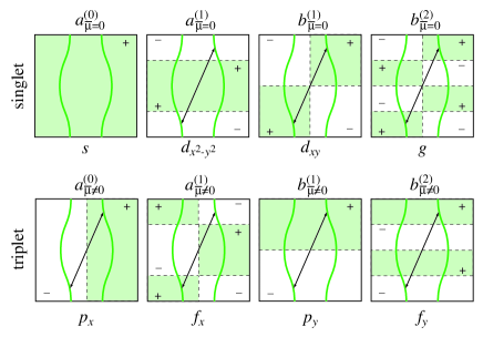
Figure 1: Types of the gap symmetry. The upper panels corresponds to the singlet pairing, whose symmetry belongs to $s$-, $d_{x^{2}-y^{2}}$-, $d_{xy}$-, $g$-wave respectively (from left to right). The lower panels corresponds to the triplet pairing, whose symmetry belongs to $p_{x}$-, $f_{x}$-, $p_{y}$-, $f_{y}$-wave respectively (from left to right). The coefficients ($a_{\bar{\mu}}^{(n)},b_{\bar{\mu}}^{(n)}$) above the panels denote the corresponding Fourier coefficients. The arrows indicate the inversion (${\bf k}\to-{\bf k}$), which does not (does) change the sign of the gap function for singlet (triplet) pairing.

3 Superconductivity vs. Density Wave

3.1 Temperature dependence of $\chi(T)$ and $T_{\rm c}$

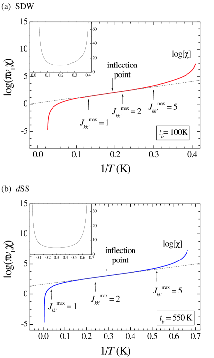
Figure 2: Response function of (a) SDW and (b) $d$SS. The dotted straight line is the line of $\tilde{\chi}_{\rm prop}$ drawn by fitting with $\tilde{\chi}$ at the inflection point. The insets show $d(\ln[\pi v_{F}\chi])/d(1/T)$ for the respective response function.

Based on the RG method derived in previous section, we examine the possible states in the present q1d system. First we calculate the response functions obtained from Eq. (32), which are shown in Fig. 2 for the SDW (a) and the $d$SS (b). Each response function (also for other response functions) shows the similarity in behavior. The important point to note is that the response function $\chi(T)$ becomes proportional to $\exp(1/T)$ (i.e., $\ln\chi(T)\propto 1/T$) in the wide region of intermediate temperatures. From the theorems of Mermin and Wagner[20], and Hohenberg[21], there is no magnetic or superconducting long-range order at any finite temperature in one and two dimensions. Generally, the response functions in two dimension have the temperature dependence $\chi(T)\propto\exp(1/T)$ for both magnetic[22] and superconducting[23, 24, 25] cases, when we do not consider the Kosterlitz-Thouless transition.[26] From these points, one may say that the present method gives a rigorous solution in such temperatures as $\chi(T)\propto\exp(1/T)$ in spite of the one-loop approximation.

In the very low temperatures, on the other hand, $\chi(T)$ strays from the behavior of $\exp(1/T)$ and diverges at finite temperature because of the divergence of the coupling $J$ or $W$. Therefore, it is appropriate to recognize the response function in the intermediate temperatures as a proper response function, since it is proportional to $\exp(1/T)$. In the region, where the obtained response function does not show the behavior of $\exp(1/T)$, the present RG technique does not work well due to the relevant (large enough) couplings. In the sense, the characteristic temperature, $T^{*}$, for the lower bound of the present RG technique, may be taken by a condition that $d(\ln[\pi v_{F}\chi])/dT^{-1}$ takes a minimum, i.e., the inflection point. In order to obtain the proper response function, we estimate by using an extrapolation formula

$$\tilde{\chi}_{\rm prop}(T)=\alpha\exp^{\beta/T},$$ (34)

where $\tilde{\chi}=\pi v_{F}\chi$. The parameter $\beta$ is defined as $\beta\equiv d(\ln[\tilde{\chi}])/dT^{-1}|_{T=T^{*}}$, which is of the order of the transition temperature obtained by the mean field approximation. The parameter $\alpha$ is defined as $\alpha\equiv\tilde{\chi}(T^{*})e^{-\beta/T^{*}}$, namely, $\tilde{\chi}_{\rm prop}(T)$ is the tangential line of $\ln\tilde{\chi}(1/T)$ at $T=T^{*}$. Assuming that the practical transition temperature $T_{\rm c}$ is lead by the three-dimensionality, we use the conventional RPA (for the inter-plane coupling), $g_{\rm 3d}\tilde{\chi}_{\rm prop}(T_{\rm c})=1$, which yields the form

$$T_{\rm c}=-\frac{\beta}{\ln(\alpha g_{\rm 3d})},$$ (35)

where $g_{\rm 3d}$ is an inter-plane coupling. Of course, we need to discuss the problem in the Kosterlitz-Thouless (KT) context in two-dimensional systems.[26] In the case of $T_{\rm c}\ll E_{F}$, however, the difference between $T_{\rm c}$ and the KT transition temperature $T_{\rm c}^{\rm KT}$ is small compared to $T_{\rm c}$, i.e., $|T_{\rm c}-T_{\rm c}^{\rm KT}|/T_{\rm c}\sim T_{\rm c}/E_{F}$.[27] Consequently, $T_{\rm c}$ determined by the present method almost corresponds to the actual transition temperature $T_{\rm c}^{\rm KT}$.

In this paper, $T_{\rm c}$ is calculated by taking $\mathcal{O}(g_{\rm 3d})\sim 10^{-3}$. We calculated $32\times 32\times 2$ simultaneous differential equations, i.e., a 32-chains system with 64 points on the Fermi surface. The initial bandwidth is set to be $E_{0}=5500K$ ($t_{a}=E_{0}/(2\sqrt{2}k_{F}^{0})\simeq 2500$K ), which is consistent with the bandwidth of (TMTSF)₂PF₆.[28, 29]

3.2 $g_{2}$-$g_{1}$ phase diagram

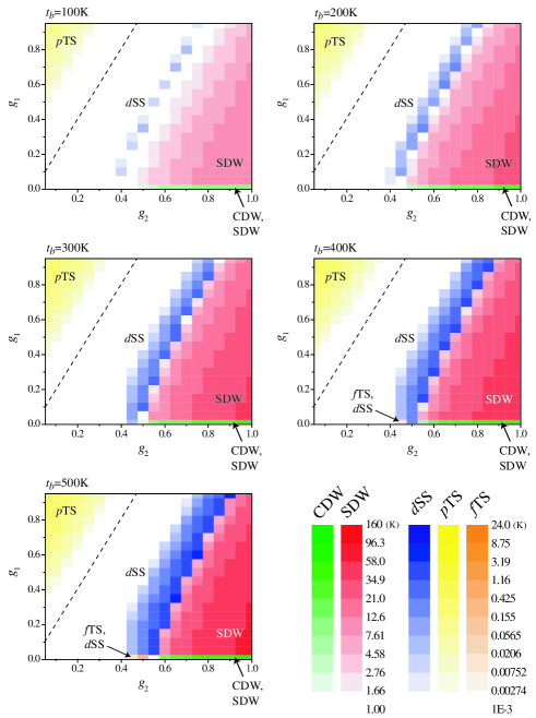
Figure 3: $g_{2}$-$g_{1}$ phase diagrams for $t_{b}=100,200,300,400$ and 500K. The transition temperatures for the CDW, SDW, $d$SS, $p$TS and $f$TS are expressed as the tones of green, red, blue, yellow and orange, respectively. The dashed-line indicates the phase boundary between the $p$TS and the SDW of the g-ology.

First, we show phase diagrams on the $g_{2}$-$g_{1}$ plane for several choices of $t_{b}$’s in order to understand the variation of the phase diagram from pure 1d case to q1d case. For repulsive interactions $g_{1,2}>0$, the SDW is dominant for $g_{1}<2g_{2}$ and the $p$-wave triplet superconductivity ($p$TS) is dominant for $g_{1}>2g_{2}$ as found in the g-ology.[17] Figure 3 shows the phase diagram for $t_{b}=$ 100, 200, 300, 400, 500K. The dashed-lines in Fig. 3 denote $g_{1}$=$2g_{2}$, which correspond to the phase boundary between the $p$TS and the SDW of the g-ology.

The present results show that the transition temperatures of the $p$TS and the SDW are extremely low (numerically, below $10^{-2}$ K) near the phase boundary $g_{1}=2g_{2}$. Moving from that line, the $p$TS and the SDW phase appears parallel to the $g_{1}$=$2g_{2}$-line. The salient feature is that, in q1d, the $d$SS phase emerges between the $g_{1}$=$2g_{2}$-line and the SDW phase, and this $d$SS phase extends to the SDW phase also parallel to $g_{1}$=$2g_{2}$, as $t_{b}$ increases. From these features, it turns out that the transition temperature depends on the intensity of $|g_{1}-2g_{2}|$, corresponding to the intensity of density fluctuations. The nearer the parameters move to the line of $g_{1}$=$2g_{2}$, the weaker the SDW instability becomes. Thus the $d$SS appears instead of the SDW state due to the deviation of the nesting condition. Just on the line of $g_{1}$=0, the CDW ($f$TS) state has the same transition temperature as the SDW ($d$SS) state. The phase boundary between the $d$SS and the normal state swerves from the line parallel to $g_{1}=2g_{2}$ for small $g_{1}$, while that between the $d$SS and the SDW is parallel to the $g_{1}$=$2g_{1}$-line. This can be understood as the interference effect of the charge fluctuations and the spin fluctuations, which shall be discussed later.

3.3 $t_{b}$-dependence of transition temperature

Next, we show $t_{b}$-dependence of the transition temperature in Fig. 4; (a) the Hubbard ($V$=0) model with $g_{1}=g_{2}=0.88$ ($U\simeq 7.8t_{a},V_{1}=V_{2}=0.0$), and (b) the extended Hubbard model with large-$V$ given by $g_{1}=0.01,g_{2}=0.55$ ($U\simeq 1.3t_{a},V_{1}\simeq 0.72t_{a}$ and $V_{2}\simeq 0.60t_{a}$, if we assume $V_{1}=1.2V_{2}$). For small $t_{b}$ ($\lesssim$300K), the transition temperature of SDW, $T_{\rm SDW}$, increases linearly. More precisely, it is approximately given by $T_{\rm SDW}\sim t_{b}\exp(-2/g_{2}^{*})$. Here, $g_{2}^{*}/2$ corresponds to the strength of the spin fluctuation, where the asterisk denotes its value at $T_{\rm cross}$. Such increase cannot be obtained by the mean field theory or the RPA-type theory, and consistent with the previous 1d RG theory;[30, 16] this feature originates from the effect of 1d fluctuation, i.e., the equally divergent contributions from both the Cooper and the Peierls channel. The transition temperature has a maximum followed by the decrease due to the nesting deviation. When $T_{\rm SDW}$ is sufficiently suppressed due to the nesting deviation, the hidden superconductivity, $d$SS in the present case, emerges. These features are seen for almost every couplings in the parameter region $0<g_{1}<2g_{2}$, corresponding to the SDW phase of the g-ology.

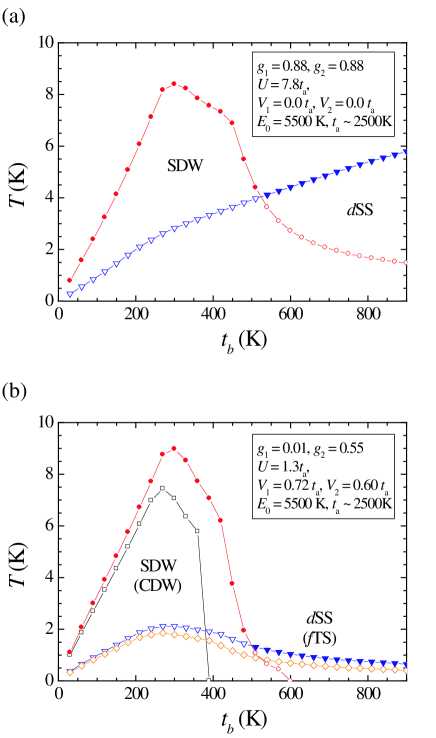
Figure 4: Transition temperature as a function of the interchain hopping $t_{b}$ for (a) the Hubbard ($V$=0) model $g_{1}=g_{2}=0.88$ ($U\simeq 7.8t_{a},V_{1}=V_{2}=0.0$), and for (b) the large-$V$ model $g_{1}=0.01,g_{2}=0.55$ ($U\simeq 1.3t_{a},V_{1}\simeq 0.72t_{a},V_{2}\simeq 0.60t_{a}$). The closed circles and triangles are the transition temperature of SDW and $d$SS, respectively. The open circles and diamonds indicates the temperature where the response functions of CDW and $f$TS satisfy the condition (35), respectively.

There are some differences between the $V$=0 and the large-$V$ model. The most noticeable difference exists in the subdominant phase for the large-$V$, which is shown by open squares (CDW) and diamonds ($f$TS) in Fig. 4 (b). Here, the transition temperature for the subdominant state are also obtained from the condition (35). The transition temperature for the subdominant CDW ($f$TS) is exactly the same as that of SDW ($d$SS) when $g_{1}=0$ ($U=2V_{2}$), i.e., just on the phase boundary between SDW and CDW of the g-ology. The actual phase transition, of course, occurs only for the most divergent response function, so that these subdominant phases are masked practically. Therefore the subdominant transition temperature is better considered as an emergence of fluctuations. In the case of large-$V$, not only the spin fluctuations but also the charge fluctuations develop, while only the spin fluctuations develop for the $V$=0. This enhancement of the charge fluctuation promotes the $f$TS state; especially, $f$TS is realized for $g_{1}=0$.

Another significant difference is that the superconducting transition temperature $T_{\rm c}$ for large-$V$ is much lower than that for $V$=0, while $T_{\rm SDW}$ of both cases are almost the same. This comes from the difference of the strength of the charge fluctuations. It is clear from the eqs. (17) and (18) that the charge fluctuation $J_{0}$ suppresses the singlet channel $W_{0}$, and enhances the triplet channel $W_{\bar{\mu}\neq 0}$. When $J_{0}=J_{\mu\neq 0}$, the amplitude of the triplet channel becomes just the same as that of singlet one, which corresponds to the $g_{1}=0$ ($U=2V_{2}$) case. Thus the low $T_{\rm c}$ of the large-$V$ model also suggests the enhancement of the charge fluctuation, which promotes the $f$TS. The $t_{b}$-dependence of $T_{\rm c}$ would be given by $T_{\rm c}\sim t_{b}\exp(-1/\tilde{g}_{\bar{\mu}}^{*})$ in the same way as the SDW. (Here, $\tilde{g}_{\bar{\mu}}^{*}$ is slightly smaller than $g_{\bar{\mu}}^{*}$ because of the nodes of the gap.) Therefore, the increasing $T_{\rm c}$ for the Hubbard model is due to the increasing $t_{b}$. The reason why $T_{\rm c}$ decreases for the large-$V$ is the rapid decrease of the spin fluctuation due to the cancellation with the charge fluctuation.

Note that the possible $f$TS state is a characteristic of systems with open-Fermi-surface such as q1d. On the other hand, in the case of the closed Fermi surface, such as the square lattice, $f$TS cannot have the comparable transition temperature even for large-$V$, but $d_{xy}$-wave singlet superconductivity can become a dominant state.[31, 32] This comes from a property of the open Fermi surface. The number of nodes of $f$TS is 4 in the case of q1d open Fermi surface, which is the same as $d$SS. Here, the number is 6 for the closed Fermi surface. Hence, the q1d system possesses a property which is favorable for the triplet pairing. As far as the pairing symmetry is concerned, the present results is consistent with the RPA results.[15] The RPA, however, does not take into account the 1d fluctuations, so that its $T_{\rm c}$ is much higher than the present one.

4 Conclusion

We have calculated the response functions and the transition temperatures for the density wave (CDW and SDW) and the superconductivity ($s$-, $p_{x}$-, $p_{y}$-, $d_{x^{2}-y^{2}}$-, $d_{xy}$-, $f_{x}$-, $f_{y}$- and $g$-wave) of q1d systems by the Kadanoff-Wilson renormalization group technique, which has been developed by Duprat and Bourbonnais.[13] The present method is able to investigate a system in pure 1d and q1d in the same footing. Each response function exhibits the temperature dependence, $\chi(T)\propto\exp(1/T)$, in a wide region of temperature, which satisfies the theorems of the Hohenberg[21], and Mermin and Wagner.[20] Also, the temperature dependence is consistent with that obtained by 2d fluctuation theories. [22, 23, 24, 25] This may suggest that the present method gives a rigorous solution to some extent.

In the phase diagram of the $g_{2}$-$g_{1}$ plane, the $p$TS and the SDW are locating in the region parallel to $g_{1}$=$2g_{2}$. The transition temperature depends on the intensity $|g_{1}-2g_{2}|$, which corresponds to the coupling constant of density-fluctuations. The $d$SS phase, which does not appear in purely 1d case, exists next to the SDW phase in q1d case. The $d$SS phase expands into the SDW region parallel to $g_{1}$=$2g_{2}$ as $t_{b}$ increases. For small $t_{b}$, $T_{\rm SDW}$ increases as $T_{\rm SDW}\sim t_{b}\exp(-2/g_{2}^{*})$. The transition temperature of the SDW has a maximum and decreases at finite $t_{b}$ ($\sim 300$K for $(g_{1},g_{2})=(0.88,0.88)$ and $(g_{1},g_{2})=(0.01,0.55)$), due to the nesting deviation. The singlet superconductivity of $d_{x^{2}-y^{2}}$-wave ($d$SS) emerges when the SDW state is suppressed by the moderately large $t_{b}$. In the large-$V$ model, the subdominant CDW ($f$-wave triplet) state is comparable to the dominant SDW ($d_{x^{2}-y^{2}}$-wave singlet) state. Especially, the transition temperature of $f$TS (CDW) becomes equivalent to that of $d$SS (SDW) with $V_{2}=U/2$. This is because the large $V$ (practically $V_{2}$) leads to the enhancement of the charge fluctuations. Such large charge-fluctuation suppresses the $d$SS and enhances the $f$TS, so that $T_{\rm c}$ of $d$SS in the large-$V$ model is much lower than that in the $V$=0 model. Consequently, the long-range Coulomb interaction can give rise to the large charge fluctuation, which suppresses $d$SS and enhances $f$TS particularly in q1d systems.

The experiments on (TMTSF)₂PF₆ compounds suggest the coexistence of $2k_{F}$-CDW and $2k_{F}$-SDW,[7, 8] and exhibit about ten times lower $T_{\rm c}$ than $T_{\rm SDW}$.[3] Considering these experimental properties, the large-$V$ model ($V_{2}/U\sim 0.5$) is appropriate for the (TMTSF)₂PF₆ compounds on the point of the phase diagram, the $2k_{F}$-charge-fluctuation in SDW phase, and the realization of the $f$TS. Actually, there is an estimation that $V_{1}/U\sim$ 0.5-0.75 ($V_{2}/U\sim$ 0.4-0.6, if we assume $V_{1}=1.2V_{2}$) on a basis of a Valence-Bond/Hartree-Fock method for molecules derived of TTF.[33]

Even if $V_{2}$ is not so large, $f$TS is possibly realized under moderately large Zeeman magnetic field, which suppresses the singlet pairing of $d$SS due to the paramagnetic effect[14]. In such a case, since the ground state is $d$SS state, the Knight shift decreases at $H=0$ but does not vary under large magnetic field. Noting that the upper critical field can be estimated as $H_{{\rm c}2}=(\Delta_{0}/\sqrt{2}\mu_{\rm B})(1-T^{2}/T_{\rm c}^{2})$,[34] we can evaluate that 1.7 T is sufficient to realize the field-induced $f$-wave triplet pairing for $T_{c}(H=0)=1.2$K, even for $T_{\rm c}^{f}\simeq T_{\rm c}^{d}/2$.[35] Here, $\Delta_{0}$ is the magnitude of the superconducting gap, and the BCS relation $2\Delta_{0}=3.5k_{\rm B}T_{\rm c}$ is assumed.

Finally, we comment on the effects of the dimerization and the Umklapp scattering, which are not considered in the present work. Following effect is expected with the Umklapp scattering $g_{3}$ as $t_{b}$ increases.[18, 36] First the Umklapp scattering causes the antiferromagnetic transition ($g_{3}$ is relevant while $g_{1}$ is irrelevant). Next, the SDW transition is realized due to the nesting property ($g_{1}$ becomes relevant). Finally, the $f$TS state results from the charge fluctuation enhanced by the off-site interaction, which is not affected by the Umklapp scattering; the essential points of the present paper would be still valid.

References

- [1] I. J. Lee, P. M. Chaikin and M. J. Naughton: Phys. Rev. Lett. 78 (1997) 3555; Phys. Rev. B 62 (2000) R14669; ibid. 65 (2002) 180502.
- [2] I. J. Lee, S. E. Brown, W. G. Clark, M. J. Strouse, M. J. Naughton, W. Kang and P. M. Chaikin: Phys. Rev. Lett. 88 (2002) 017004; I. J. Lee, D. S. Chow, W. G. Clark, M. J. Strouse, M. J. Naughton, P. M. Chaikin and S. E. Brouwn: Phys. Rev. B 68 (2003) 092510.
- [3] D. Jerome: Mol. Cryst. Liq. Cryst. 79 (1982) 155.
- [4] K. Miyake, S. Schmitt-Rink and C. M. Varma: Phys. Rev. B 34 (1986) 6554.
- [5] D. J. Scalapino, E. Loh, Jr. and J. E. Hirsch: Phys. Rev. B 34 (1986) 8190.
- [6] V. J. Emery: Synthetic Metals 13 (1986) 21.
- [7] J. P. Pouget and S. Ravy: J. Phys. I 6 (1996) 1501.
- [8] S. Kagoshima, Y. Saso, M. Maesato, R. Kondo and T. Hasegawa: Solid State Comm. 110 (1999) 479.
- [9] H. Shimahara: J. Phys. Soc. Jpn. 58 (1989) 1735.
- [10] H. Kino and H. Kontani: J. Phys. Soc. Jpn. 68 (1999) 1481.
- [11] K. Kuroki, R. Arita and H. Aoki: Phys. Rev. B 63 (2001) 094509.
- [12] T. Nomura and K. Yamada: J. Phys. Soc. Jpn. 70 (2001) 2694.
- [13] R. Duprat and C. Bourbonnais: Eur. Phys. J. B 21 (2001) 219.
- [14] Y. Fuseya, Y. Onishi, H. Kohno and K. Miyake: J. Phys.: Condens. Matter 14 (2002) L655.
- [15] Y. Tanaka and K. Kuroki: Phys. Rev. B 70 (2004) 060502(R).
- [16] C. Bourbonnais and L. G. Caron: Int. J. Mod. Phys. B 5 (1991) 1033; C. Bourbonnais, B. Guay and R. Wortis: in Theoretical Methods for Strongly Correlated Electrons ed. D. Snchal, A. M. Tremblay and C. Bourbonnais (Springer-Verlag, New York, 2004) p. 77.
- [17] See, for example, J. Solyom: Adv. Phys. 28 (1979) 201.
- [18] J. Kishine and K. Yonemitsu: J. Phys. Soc. Jpn. 67 (1998) 2590; ibid 68 (1999) 2790.
- [19] Of course, in q1d systems, we cannot classify the gap symmetry by the spherical-wave basis or the irreducible representation of the tetragonal. Here, we use an idiomatic representation such as -, -, , and displayed in Fig. 1.
- [20] N. D. Mermin and H. Wagner: Phys. Rev. Lett. 17 (1966) 1133.
- [21] P. C. Hohenberg: Phys. Rev. 158 (1967) 383.
- [22] See, for example, J. M. Kosterlitz and D. J. Thouless: in Progress in Low Temperature Physics VII B, ed. D. F. Brewer (North-Holland, Amsterdam, 1978) p. 371.
- [23] A. Tokumitu, K. Miyake and K. Yamada: J. Phys. Soc. Jpn. 60 (1991) 380.
- [24] private communication with K. Miyake.
- [25] Y. Kosuge, A. Kobayashi, T. Matsuura and Y. Kuroda: J. Phys. Soc. Jpn. 72 (2003) 1166; Y. Kosuge: doctoral thesis, Nagoya University, (2003).
- [26] J. M. Kosterlitz and D. Thouless: J. Phys. C6 (1973) 1181; J. M. Kosterlitz: ibid. C7 (1974) 1046.
- [27] K. Miyake: Prog. Theor. Phys. 69 (1983) 1794.
- [28] C. S. Jacobsen, D. B. Tanner and K. Bechgaard: Phys. Rev. B 28 (1983) 7019.
- [29] P. M. Grant: J. Physique 44 (1983) C3-847.
- [30] Y. Suzumura and H. Fukuyama: J. Low Temp. Phys. 31 (1978) 273.
- [31] S. Onari, R. Arita, K. Kuroki and H. Aoki: cond-mat/0312314.
- [32] A. Kobayashi, Y. Tanaka, M. Ogata and Y. Suzumura: J. Phys. Soc. Jpn. 73 (2004) 1115.
- [33] F. Castet, A. Fritsch and L. Ducasse: J. Phys. I France, 6 (1996) 583.
- [34] A. M. Clogston: Phys. Rev. Lett. 9 (1962) 266.
- [35] The evaluated Zeeman magnetic field here is the magnetic field where the singlet pairings are completely broken. The reversal from SS to TS is expected below the of the SS.
- [36] C. Bourbonnais and R. Duprat: J. Phys. IV France, 114 (2004) 3.