Response of discrete nonlinear systems with many degrees of freedom

Abstract

We study the response of a large array of coupled nonlinear oscillators to parametric excitation, motivated by the growing interest in the nonlinear dynamics of microelectromechanical and nanoelectromechanical systems (MEMS and NEMS). Using a multiscale analysis, we derive an amplitude equation that captures the slow dynamics of the coupled oscillators just above the onset of parametric oscillations. The amplitude equation that we derive here from first principles exhibits a wavenumber dependent bifurcation similar in character to the behavior known to exist in fluids undergoing the Faraday wave instability. We confirm this behavior numerically and make suggestions for testing it experimentally with MEMS and NEMS resonators.

I Motivation

In the last decade we have witnessed exciting technological advances in the fabrication and control of microelectromechanical and nanoelectromechanical systems (MEMS and NEMS). Such systems are being developed for a host of nanotechnological applications, as well as for basic research in the mesoscopic physics of phonons, and the general study of the behavior of mechanical degrees of freedom at the interface between the quantum and the classical worlds Roukes (2001); Cleland (2003); Blencowe (2004). Surprisingly, NEMS have also opened up a new experimental window into the study of the nonlinear dynamics of discrete systems with many degrees of freedom. A combination of three properties of NEMS resonators has led to this unique experimental opportunity. First and most important is the experimental observation that micro- and nanomechanical resonators tend to behave nonlinearly at very modest amplitudes. This nonlinear behavior has not only been observed experimentally Turner et al. (1998); Craighead (2000); Buks and Roukes (2001); Scheible et al. (2002); Zhang et al. (2002, 2003); Yu et al. (2002); Aldridge and Cleland (2005), but has already been exploited to achieve mechanical signal amplification and mechanical noise squeezing Rugar and Grütter (1991); Carr et al. (2000) in single resonators. Second is the fact that at their dimensions, the normal frequencies of nanomechanical resonators are extremely high—recently exceeding the 1GHz mark Huang et al. (2003); Cleland and Geller (2004)—facilitating the design of ultra-fast mechanical devices, and making the waiting times for unwanted transients bearable on experimental time scales. Third is the technological ability to fabricate large arrays of MEMS and NEMS resonators whose collective response might be useful for signal enhancement and noise reduction Cross et al. (2004), as well as for sophisticated mechanical signal processing applications. Such arrays have already exhibited interesting nonlinear dynamics ranging from the formation of extended patterns Buks and Roukes (2002)—as one commonly observes in analogous continuous systems such as Faraday waves—to that of intrinsically localized modes Sato et al. (2003a, b, 2004). Thus, nanomechanical resonator arrays are perfect for testing dynamical theories of discrete nonlinear systems with many degrees of freedom. At the same time, the theoretical understanding of such systems may prove useful for future nanotechnological applications.

Two of us (Lifshitz and Cross (Lifshitz and Cross, 2003, henceforth LC)) have recently studied the response of coupled nonlinear oscillators to parametric excitation. We used secular perturbation theory to convert the equations of motion for the oscillators into a set of coupled nonlinear algebraic equations for the normal mode amplitudes of the system, enabling us to obtain exact results for small arrays but only a qualitative understanding of the dynamics of large arrays. In order to obtain analytical results for large arrays we study here the same system of equations, approaching it from the continuous limit of infinitely-many degrees of freedom. A novel feature of the paramerically driven instability is that the bifurcation to standing waves switches from supercritical (second order) to subcritical (first order) at a wave number at or close to the critical one for which the required driving force is minimum. This changes the form of the amplitude equation that describes the onset of the paramerically driven waves so that it no longer has the standard “Ginzburg-Landau” form. Our central result is this new scaled amplitude equation (21), governed by a single control parameter, that captures the slow dynamics of the coupled oscillators just above the onset of parametric oscillations including this unusual bifurcation behavior. We confirm the behavior numerically and make suggestions for testing it experimentally. Although our focus is on parametrically driven oscillators, the amplitude equation we derive should also apply to other parametrically driven wave systems with weak nonlinear damping.

II Equations of Motion

The equations of motion introduced in LC are

$$\ddot{u}_{n} +u_{n}+u_{n}^{3}-\frac{1}{2}\Gamma(\dot{u}_{n+1}-2\dot{u}_{n}+\dot{u}_{n-1})$$

$$+\frac{1}{2}\Delta^{2}\bigl{[}1+H\cos(2\omega_{p}t)\bigr{]}(u_{n+1}-2u_{n}+u_{n-1})$$

$$-\frac{1}{2}\eta\bigl{[}(u_{n+1}-u_{n})^{2}(\dot{u}_{n+1}-\dot{u}_{n})$$

$$-(u_{n}-u_{n-1})^{2}(\dot{u}_{n}-\dot{u}_{n-1})\bigr{]}=0,$$ (1)

with $n=1\ldots N$, and fixed boundary conditions $u_{0}=u_{N+1}=0$. The equations of motion (II) are modeled after the experiment of Buks and Roukes Buks and Roukes (2002), who succeeded in fabricating, exciting, and measuring the response to parametric excitation of an array of 67 micromechanical resonating gold beams. Detailed arguments for the choice of terms introduced into the equations of motion are given by LC. The guiding principle is to introduce only those terms that are essential for capturing the physical behavior observed in the experiment. These include a cubic nonlinear elastic restoring force (whose coefficient is scaled to 1), a dc electrostatic nearest-neighbor coupling term with a small ac component responsible for the parametric excitation (with coefficients $\Delta^{2}$ and $\Delta^{2}H$ respectively), and linear as well as cubic nonlinear dissipation terms (with coefficients $\Gamma$ and $\eta$ respectively). The nonlinear contribution to the dissipation, though expected to be small, is essential for the saturation of the amplitude of the parametrically driven motion Lifshitz and Cross (2003) and is important in the behavior of the bifircation as a function of wave number. Both dissipation terms are taken to be of a nearest neighbor form, motivated by the experimental indication that most of the dissipation comes from the electrostatic interaction between neighboring beams. It should be noted that the effect of introducing gradient-dependent dissipation terms instead of local dissipation terms is merely to renormalize the bare dissipation coefficients $\Gamma$ and $\eta$ to wavenumber-dependent coefficients of the form $\Gamma\sin^{2}\left(q/2\right)$ and $\eta\sin^{2}\left(q/2\right)$ respectively, as will become apparent below.

The dissipation of the system is assumed to be weak, which makes it possible to excite the beams with relatively small driving amplitudes. In such case the response of the beams is moderate, justifying the description of the system with nonlinearities up to cubic terms only. The weak dissipation can be parameterized by introducing a small expansion parameter $\epsilon\ll 1$, physically defined by the linear dissipation coefficient $\Gamma\equiv\epsilon\gamma$, with $\gamma$ of order one. The driving amplitude is then expressed by $\Delta^{2}H=\epsilon h$, with $h$ of order one. We assume the system is excited in its first instability tongue, i.e. we take $\omega_{p}$ itself to lie within the normal frequency band $\sqrt{1-2\Delta^{2}}<\omega_{p}<1$. The weakly nonlinear regime is studied by expanding the displacements $u_{n}$ in powers of $\epsilon$. Taking the leading term to be of the order of $\epsilon^{1/2}$ ensures that all the corrections, to a simple set of equations describing $N$ coupled harmonic oscillators, enter the equations at the same order of $\epsilon^{3/2}$.

III Amplitude Equations for Counter Propagating Waves

We introduce a continuous displacement field $u(x,t)$, keeping in mind that only for integral values $x=n$ of the spatial coordinate does it actually correspond to the displacements $u(n,t)=u_{n}(t)$ of the discrete set of oscillators in the array. We introduce slow spatial and temporal scales, $X=\epsilon x$ and $T=\epsilon t$, upon which the dynamics of the envelope function occurs, and expand the displacement field in terms of $\epsilon$,

$$u(x,t) = \epsilon^{1/2}\bigl{[}\left(A_{+}(X,T)e^{-iq_{p}x}+A_{-}^{*}(X,T)e^{iq_{p}x}\right)e^{i\omega_{p}t}$$ (2)

$$+ c.c.\bigr{]}+\epsilon^{3/2}u^{(1)}(x,t,X,T)+\ldots,$$

where the asterisk and $c.c.$ stand for the complex conjugate, and $q_{p}$ and $\omega_{p}$ are related through the dispersion relation $\omega_{p}^{2}=1-2\Delta^{2}\sin^{2}(q_{p}/2)$. The response to lowest order in $\epsilon$ is expressed in terms of two counter-propagating waves with complex amplitudes $A_{+}$ and $A_{-}$, a typical ansatz for parametrically excited continuous systems Cross and Hohenberg (1993). We substitute the ansatz (2) into the equations of motion (II) term by term. Up to order $\epsilon^{3/2}$, we have

$$\ddot{u}_{n} =-\epsilon^{1/2}\omega_{p}^{2}\left(A_{+}(X,T)e^{-iq_{p}x}+A_{-}^{*}(X,T)e^{iq_{p}x}\right)e^{i\omega_{p}t}+\epsilon^{3/2}\frac{\partial^{2}u^{(1)}}{\partial t^{2}}(x,t,X,T)$$

$$+\epsilon^{3/2}2i\omega_{p}\left(\frac{\partial A_{+}(X,T)}{\partial T}e^{-iq_{p}x}+\frac{\partial A_{-}^{*}(X,T)}{\partial T}e^{iq_{p}x}\right)e^{i\omega_{p}t}+c.c.\,;$$ (3a)

$$u_{n\pm 1} =\epsilon^{1/2}\left(A_{+}(X,T)e^{-iq_{p}(x\pm 1)}+A_{-}^{*}(X,T)e^{iq_{p}(x\pm 1)}\right)e^{i\omega_{p}t}+\epsilon^{3/2}u^{(1)}(x\pm 1,t,X,T)$$

$$\pm\epsilon^{3/2}\left(\frac{\partial A_{+}}{\partial X}e^{-iq_{p}x}e^{\mp iq_{p}}+\frac{\partial A_{-}^{*}}{\partial X}e^{iq_{p}x}e^{\pm iq_{p}}\right)e^{i\omega_{p}t}+c.c.\,;$$ (3b)

$$\frac{1}{2}\Delta^{2} \left(u_{n+1}-2u_{n}+u_{n-1}\right)=-\epsilon^{1/2}2\Delta^{2}\sin^{2}(q_{p}/2)\left(A_{+}e^{-iq_{p}x}+A_{-}^{*}e^{iq_{p}x}\right)e^{i\omega_{p}t}$$

$$+\epsilon^{3/2}\left(u^{(1)}(x+1,t,X,T)-2u^{(1)}(x,t,X,T)+u^{(1)}(x-1,t,X,T)\right)$$

$$-\epsilon^{3/2}\Delta^{2}i\sin(q_{p})\left(\frac{\partial A_{+}}{\partial X}e^{-iq_{p}x}-\frac{\partial A_{-}^{*}}{\partial X}e^{iq_{p}x}\right)e^{i\omega_{p}t}+c.c.\,;$$ (3c)

$$\frac{1}{2}\epsilon h{\rm c} {\rm os}(2\omega_{p}t)(u_{n+1}-2u_{n}+u_{n-1})=-\epsilon^{3/2}h\sin^{2}(q_{p}/2)\left(A_{-}e^{-iq_{p}x}+A_{+}^{*}e^{iq_{p}x}\right)e^{i\omega_{p}t}+O(e^{i3\omega_{p}t})+c.c.\,;$$ (3d)

$$\frac{1}{2}\epsilon\gamma( \dot{u}_{n+1}-2\dot{u}_{n}+\dot{u}_{n-1})=-\epsilon^{3/2}2i\gamma\omega_{p}\sin^{2}(q_{p}/2)\left(A_{+}e^{-iq_{p}x}+A_{-}^{*}e^{iq_{p}x}\right)e^{i\omega_{p}t}+c.c.\,;$$ (3e)

$$u_{n}^{3}= \epsilon^{3/2}3\left[(|A_{+}|^{2}+2|A_{-}|^{2})A_{+}e^{-iq_{p}x}+(2|A_{+}|^{2}+|A_{-}|^{2})A_{-}^{*}e^{iq_{p}x}\right]e^{i\omega_{p}t}+O\left(e^{i3\omega_{p}t},e^{i3q_{p}x}\right)+c.c.\,;$$ (3f)

$$\frac{1}{2}\eta\left[\vphantom{\dot{u}_{n}}\right.( \left.u_{n+1}-u_{n})^{2}(\dot{u}_{n+1}-\dot{u}_{n})-(u_{n}-u_{n-1})^{2}(\dot{u}_{n}-\dot{u}_{n-1})\right]=-\epsilon^{3/2}i8\eta\omega_{p}\sin^{4}(q_{p}/2)$$

$$\times\left[(|A_{+}|^{2}+2|A_{-}|^{2})A_{+}e^{-iq_{p}x}+(2|A_{+}|^{2}+|A_{-}|^{2})A_{-}^{*}e^{iq_{p}x}\right]e^{i\omega_{p}t}+O(e^{i3\omega_{p}t},e^{i3q_{p}x})+c.c.\,,$$ (3g)

where $O(e^{i3\omega_{p}t},e^{i3q_{p}x})$ are terms proportional to $e^{i3\omega_{p}t}$ or $e^{i3q_{p}x}$ which do not enter the dynamics at the lowest order of the $\epsilon$ expansion. At the order of $\epsilon^{1/2}$, the equations of motion (II) are satisfied trivially, yielding the dispersion relation mentioned earlier. At the order of $\epsilon^{3/2}$ on the other hand we must apply a solvability condition Cross and Hohenberg (1993), which requires that all terms proportional to $e^{(i\omega_{p}t\pm q_{p}x)}$ must vanish. We therefore obtain the two coupled amplitude equations,

$$\frac{\partial A_{\pm}}{\partial T} \pm v_{g}\frac{\partial A_{\pm}}{\partial X}=-\gamma\sin^{2}\left(\frac{q_{p}}{2}\right)A_{\pm}\mp i\frac{h}{2\omega_{p}}\sin^{2}\left(\frac{q_{p}}{2}\right)A_{\mp}$$ (4)

$$- \left(4\eta\sin^{4}\left(\frac{q_{p}}{2}\right)\mp i\frac{3}{2\omega_{p}}\right)\left(|A_{\pm}|^{2}+2|A_{\mp}|^{2}\right)A_{\pm},$$

where the upper signs (lower signs) give the equation for $A_{+}$ ($A_{-}$) obtained from the restriction on the terms proportional to $e^{(i\omega_{p}t-q_{p}x)}$ ($e^{(i\omega_{p}t+q_{p}x)}$), and

$$v_{g}=\frac{\partial\omega}{\partial q}=-\frac{\Delta^{2}\sin(q_{p})}{2\omega_{p}}$$ (5)

is the group velocity. A detailed derivation of the amplitude equations (4) can be found in Ref. Bromberg, 2004. Similar equations were previously derived for describing Faraday waves Ezerskiĭ et al. (1986); Milner (1991).

IV Reduction to a Single Amplitude Equation

By linearizing the amplitude equations (4) about the zero solution ($A_{+}=A_{-}=0$) we find that the linear combination of the two amplitudes that first becomes unstable at $h=2\gamma\omega_{p}$ is $B\propto(A_{+}-iA_{-})$—representing the emergence of a standing wave with a temporal phase of $\pi/4$ relative to the drive—while the orthogonal linear combination of the amplitudes decays exponentially and does not participate in the dynamics at onset. Thus, just above threshold we can reduce the description of the dynamics to a single amplitude $B$, where at a finite amplitude above threshold a band of unstable modes around $q_{p}$ can contribute to the spatial form of $B$. This is similar to the procedure introduced by Riecke Riecke (1990) for describing the onset of Faraday waves.

In the absence of nonlinear damping $\eta=0$ the coefficient of the nonlinear term in Eq. (4) is purely imaginary. This turns out to yield the result that there is no nonlinear saturation term of the usual form $\left|B\right|^{2}B$ for the standing waves at the resonant wave vector $q_{p}$. An analysis of the saturation of standing waves of nearby wave numbers $q_{p}+k$ for this case shows that the coefficient of $\left|B_{k}\right|^{2}B_{k}$ is positive for $k<0$, zero at $k=0$, and negative for $k>0.$This means that for $\eta=0$ the nature of the bifurcation to standing waves switches from supercritical to subcritical precisely at the critical wave number $q=q_{p}$. Thus the amplitude equation describing the onset of the standing waves will not be of the usual Ginzburg-Landau form. It is the goal of the present section to derive the novel form of the amplitude equation. We will do this for the case of $\eta$ small but non-zero, in which case the switch from subcritical to supercritical occurs at a wave number close to the resonant wave number $q_{p}$.

We define a reduced driving amplitude $g$ with respect to the threshold $2\gamma\omega_{p}$ by letting $(h-2\gamma\omega_{p})/2\gamma\omega_{p}\equiv g\delta$, with $\delta\ll 1$. In order to obtain an equation, describing the relevant slow dynamics of the new amplitude $B$, we need to select the proper scaling of the original amplitudes $A_{\pm}$, as well as their spatial and temporal variables, with respect to the new small parameter $\delta$. We assume that the coefficient of nonlinear dissipation $\eta$ is small. As we have seen, for some wave numbers near $q_{p}$ the bifurcation is then subcritical, so that a quintic term must enter in order to saturate the growth of the amplitude. This is similar to the situation encountered by Deissler and Brand Deissler and Brand (1998) who studied localized modes near a subcritical bifurcation to traveling waves. Here this can be achieved by defining the small parameter $\delta$ with respect to the coefficient of nonlinear dissipation—letting $\eta=\delta^{1/2}\eta_{0}$, with $\eta_{0}$ of order one—and taking the amplitudes to be of order $\delta^{1/4}$. Further noting that with a drive amplitude that scales as $\delta$ the growth rate scales like $\delta$ as well, and the bandwidth of unstable wave numbers scales as $\delta^{1/2}$, we finally make the ansatz that

$$\left(\begin{array}[]{c}A_{+}\\ A_{-}\\ \end{array}\right) = \delta^{1/4}\left(\begin{array}[]{c}1\\ i\\ \end{array}\right)B(\hat{\xi},\hat{\tau})+\delta^{3/4}\left(\begin{array}[]{c}w^{(1)}(X,T,\hat{\xi},\hat{\tau})\\ v^{(1)}(X,T,\hat{\xi},\hat{\tau})\\ \end{array}\right)$$ (12)

$$+ \delta^{5/4}\left(\begin{array}[]{c}w^{(2)}(X,T,\hat{\xi},\hat{\tau})\\ v^{(2)}(X,T,\hat{\xi},\hat{\tau})\\ \end{array}\right),$$ (15)

where $\hat{\xi}=\delta^{1/2}X$ and $\hat{\tau}=\delta T$ are the new spatial and temporal scales respectively. The amplitude equation for $B(\hat{\xi},\hat{\tau})$ is derived by once again using the multiple scales method. We substitute the ansatz (12) into the coupled amplitude equations (4) and collect terms of different orders of $\delta$.

Again, to the lowest order of expansion the equations are satisfied trivially. Collecting all terms of order $\delta^{3/4}$ in Eqs. (4) yields

$$\mathfrak{O}\left(\begin{array}[]{c}w^{(1)}\\ v^{(1)}\\ \end{array}\right)=\left(-v_{g}\frac{\partial B}{\partial\hat{\xi}}+i\frac{9}{2\omega_{p}}|B|^{2}B\right)\left(\begin{array}[]{c}1\\ -i\\ \end{array}\right),$$ (16)

where $\mathfrak{O}$ is a linear operator given by the matrix

$$\left(\begin{array}[]{cc}\partial_{T}+v_{g}\partial_{X}+\gamma\sin^{2}(q_{p}/2)&i\gamma\sin^{2}(q_{p}/2)\\ -i\gamma\sin^{2}(q_{p}/2)&\partial_{T}-v_{g}\partial_{X}+\gamma\sin^{2}(q_{p}/2)\\ \end{array}\right).$$ (17)

There is no solvability condition to satisfy here because the right hand side of Eq. (16) is automatically orthogonal to the zero eigenvalue of $\mathfrak{O}$, $\scriptsize\left(\begin{array}[]{c}1\\ i\\ \end{array}\right)$. The solution of Eq. (16) is given by

$$\begin{split}&\left(\begin{array}[]{c}w^{(1)}\\ v^{(1)}\\ \end{array}\right)=\\ &\frac{1}{2\gamma\sin^{2}(q_{p}/2)}\left(-v_{g}\frac{\partial B}{\partial\hat{\xi}}+i\frac{9}{2\omega_{p}}|B|^{2}B\right)\left(\begin{array}[]{c}1\\ -i\\ \end{array}\right).\end{split}$$ (18)

We plug Eq. (18) back into Eqs. (4), collect all the terms of order $\delta^{5/4}$ and obtain

$$\mathfrak{O}\left(\begin{array}[]{c}w^{(2)}\\ v^{(2)}\\ \end{array}\right)=\left[-\frac{\partial B}{\partial\hat{\tau}}+\frac{v_{g}^{2}}{2\gamma\sin^{2}(q_{p}/2)}\frac{\partial^{2}B}{\partial\hat{\xi}^{2}}+\gamma\sin^{2}(q_{p}/2)gB-12\eta_{0}\sin^{4}(q_{p}/2)|B|^{2}B\vphantom{1}\right.\\ +i\frac{3(-v_{g})}{2\omega_{p}\gamma\sin^{2}(q_{p}/2)}\left(4|B|^{2}\frac{\partial B}{\partial\hat{\xi}}+B^{2}\frac{\partial B^{*}}{\partial\hat{\xi}}\right)-\frac{81}{8\omega_{p}^{2}\gamma\sin^{2}(q_{p}/2)}|B|^{4}B\left.\vphantom{\frac{1}{2}}\right]\left(\begin{array}[]{c}1\\ i\\ \end{array}\right).$$ (19)

The solvability condition of Eq. (19), stating that the zero eigenvalue of the operator $\mathfrak{O}$, $\scriptsize\left(\begin{array}[]{c}1\\ i\\ \end{array}\right)$, must be orthogonal to the right hand side of the equation, determines the amplitude equation for $B$ Cross and Hohenberg (1993). Thus, the expression in square brackets in Eq. (19) must vanish. After applying one last set of rescaling transformations,

$$\hat{\tau} = \frac{9}{32}\frac{\tau}{\omega_{p}^{2}\eta_{0}^{2}\gamma\sin^{10}\left({q_{p}/2}\right)},\quad\hat{\xi}=\frac{3}{8}\frac{|v_{g}|\xi}{\omega_{p}\eta_{0}\gamma\sin^{6}\left({q_{p}/2}\right)},$$ (20)

$$|B|^{2}\rightarrow\frac{16}{27}\omega_{p}^{2}\eta_{0}\gamma\sin^{6}\left(\frac{q_{p}}{2}\right)|B|^{2},$$

$$g\rightarrow\frac{32}{9}\omega_{p}^{2}\eta_{0}^{2}\sin^{8}\left(\frac{q_{p}}{2}\right)g,$$

we end up with an amplitude equation governed by a single parameter,

$$\frac{\partial B}{\partial\tau} = gB+\frac{\partial^{2}B}{\partial\xi^{2}}+i\frac{2}{3}\left(4|B|^{2}\frac{\partial B}{\partial\xi}+B^{2}\frac{\partial B^{*}}{\partial\xi}\right)$$ (21)

$$-2|B|^{2}B-|B|^{4}B.$$

Note that Eq. (21) is a scaled equation with all coefficients of order unity. In an equation for the unscaled mode amplitude $\tilde{B}=\delta^{1/4}B$ (i.e. the combination of $A_{+},A_{-}$ that goes unstable) and using the length and time variables $X,T$ rather than $\xi,\tau$, the coefficient of the cubic saturation term $|\tilde{B}|^{2}\tilde{B}$ would be small, scaling as $\delta^{1/2}$, reflecting its origin in the nonlinear damping term, the linear growth term proportional to $\tilde{B}$ would have a coefficient scaling as $(h-h_{c})/h_{c}$, and all other coefficients would be of order unity. All terms in the equation are then of comparable size for $(h-h_{c})/h_{c}\sim\delta$, for oscillation amplitudes $\tilde{B}\sim\delta^{1/4}$, and for length scales $X\sim\delta^{-1/2}$ and time scales $T\sim\delta^{-1}$. The form of Eq. (21) is also applicable to the onset of parametrically driven standing waves in continuum systems with weak nonlinear damping, and combines in a single equation a number of effects studied previously Ezerskiĭ et al. (1986); Milner (1991); Riecke (1990); Deissler and Brand (1998); Chen and Wu (2000); Chen (2002). The numerical coefficients in the variable scalings and in the equation will, of course, be different for different systems.

Once we have obtained this amplitude equation it can be used to study a variety of dynamical solutions, ranging from simple single-mode to more complicated nonlinear extended solutions, or possibly even localized solutions.

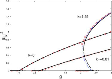
Figure 1: (Color online) Response of the oscillator array plotted as a function of reduced amplitude $g$ for three different scaled wave number shifts determined by fixing the number of oscillators $N$: $k=0$ (for $N=100$) and $k=-0.81$ (for $N=92$), which bifurcate supercritically, and $k=1.55$ (for $N=98$) which bifurcates subcritically showing clear hysteresis. Solid and dashed lines are the positive and negative square root branches of the calculated response in (23), the latter clearly unstable. Open circles are numerical values obtained by integration of the equations of motion (II) for each $N$, with $\Delta=0.5$, $\omega_{p}=0.767445$, $\epsilon\gamma=0.01$, and $\eta=0.1$. For these parameters a unity of the scaled squared amplitude $|b_{k}|^{2}$ corresponds to $2\;10^{-4}$ for the unscaled squared amplitude, and a unity of the wave number shift $k$ corresponds to a shift of $9\;10^{-3}$ of the unscaled wavenumber. Dots show the subcritically-bifurcating single-mode solution of LC Lifshitz and Cross (2003).

V Single Mode Oscillations

In this section we begin the investigation of the solutions of Eq. (21) by focusing on the regime of small reduced drive amplitude $g$ and look upon the saturation of single-mode solutions of the form

$$B=b_{k}e^{-ik\xi},$$ (22)

corresponding—via the scaling $\hat{\xi}=S_{\xi}\xi$, where the scale factor $S_{\xi}$ is defined in (20)—to a standing wave with a shifted wave number $q=q_{p}+k\epsilon\sqrt{\delta}/S_{\xi}$. From the linear terms in the amplitude equation (21) we find, as expected, that for $g>k^{2}$ the zero-displacement solution is unstable to small perturbations of the form of (22), defining the parabolic neutral stability curve, shown as a dashed line in Fig. 2. The nonlinear gradients and the cubic term take the simple form $2(k-1)|b_{k}|^{2}b_{k}$. For $k<1$ these terms immediately act to saturate the growth of the amplitude assisted by the quintic term. Standing waves therefore bifurcate supercritically from the zero-displacement state. For $k>1$ the cubic terms act to increase the growth of the amplitude, and saturation is achieved only by the quintic term. Standing waves therefore bifurcate subcritically from the zero-displacement state. Note that wave-number dependent bifurcations similar in character were also predicted and observed numerically in Faraday waves Milner (1991); Chen and Wu (2000); Chen (2002). The saturated amplitude $|b_{k}|$, obtained by setting Eq. (21) to zero, is given by

$$|b_{k}|^{2}=(k-1)\pm\sqrt{(k-1)^{2}+(g-k^{2})}\geq 0.$$ (23)

The original boundary conditions $u(0,t)=u(N+1,t)=0$ impose a phase of $\pi/4$ on $b_{k}$ and require that the wave numbers be quantized $q_{m}=m\pi/(N+1)$, $m=1\ldots N$.

In Fig. (1) we plot $|b_{k}|^{2}$ as a function of the reduced driving amplitude $g$ for three different wave number shifts $k$. The solid (dashed) lines are the stable (unstable) solutions of Eq. (23). The circles were obtained by numerical integration of the equations of motion (II). For each driving amplitude, the Fourier components of the steady state solution were computed to verify that only single modes are found, suggesting that in this regime of parameters only these states are stable. By changing the number $N$ of oscillators we could control the wave number shift $k$ for a fixed value of $\omega_{p}$. In experiment it might be easier to control $k$, for a fixed value of $\omega_{p}$, by changing the dc component of the potential difference between the beams, thus changing the dispersion relation and with it the value of $q_{p}$.

Lifshitz and Cross (Lifshitz and Cross, 2003, Eq. (33)) obtained the exact form of single mode solutions by substituting $u_{n}=A_{m}\sin(q_{m}n)e^{i\omega_{p}t}+c.c$ directly into the equations of motion (II). In the limit of driving amplitudes just above threshold and $\eta\ll 1$ their solution corresponds to Eq. (23), as shown by the dots in Fig. (1). In order to compare the two solutions one should note that in both cases the system oscillates in one of its normal modes $q_{m}$ with the driving frequency $\omega_{p}$. Here we use $k$ to denote the difference between $q_{p}$ and the wavenumber of the oscillating pattern, whereas Lifshitz and Cross use a frequency detuning $\omega_{p}-\omega_{m}$ to denote the difference between the normal frequency and the actual frequency of the oscillations. The frequency detuning $\omega_{p}-\omega_{m}$ is proportional to $v_{g}k\epsilon\sqrt{\delta}$, implying that for an infinitly extended system the standing waves will always bifurcate supercritically with a wave number $q_{p}$ if the driving amplitude is increased quasistatically. It is the discreteness of the normal modes which provides the detuning essential for a subcritical bifurcation if only quasistatic changes are performed.

VI Secondary Instabilities

We study secondary instabilities of the single mode solutions by performing linear stability analysis of (22). We substitute

$$B(\xi,\tau)=b_{k}e^{-ik\xi}+\left(\beta_{+}(\tau)e^{-i(k+Q)\xi}+\beta_{-}^{*}(\tau)e^{-i(k-Q)\xi}\right),$$ (24)

with $|\beta_{\pm}|\ll 1$, into the amplitude equation (21) and linearize in $\beta_{\pm}$. Since the amplitude equation (21) is invariant under phase transformations $B\rightarrow Be^{-i\varphi}$, the stability of the single mode solution cannot depend on the phase of $b_{k}$. We therefore assume that $b_{k}$ is real, and linearize the following terms of Eq. (21)

$$|B|^{2}B \rightarrow e^{-ik\xi}\left(b_{k}^{3}+b_{k}^{2}\left((2\beta_{+}+\beta_{-})e^{-iQ\xi}+(\beta_{+}^{*}+2\beta_{-}^{*})e^{iQ\xi}\right)\right)\,;$$

$$|B|^{4}B \rightarrow e^{-ik\xi}\left(b_{k}^{5}+b_{k}^{4}\left((3\beta_{+}+2\beta_{-})e^{-iQ\xi}+(2\beta_{+}^{*}+3\beta_{-}^{*})e^{iQ\xi}\right)\right)\,;$$

$$|B|^{2}\frac{\partial B}{\partial\xi} \rightarrow e^{-ik\xi}\left(-ikb_{k}^{3}-ib_{k}^{2}\left(((2k+Q)\beta_{+}+k\beta_{-})e^{-iQ\xi}+(k\beta_{+}^{*}+(2k-Q)\beta_{-}^{*})e^{iQ\xi}\right)\right)\,;$$

$$B^{2}\frac{\partial B^{*}}{\partial\xi} \rightarrow e^{-ik\xi}\left(ikb_{k}^{3}+ib_{k}^{2}\left((2k\beta_{+}+(k-Q)\beta_{-})e^{-iQ\xi}+((k+Q)\beta_{+}^{*}+2k\beta_{-}^{*})e^{iQ\xi}\right)\right).$$

The terms of order one of the equation obtained from the linearization of Eq. (21) recover the same Eq. (23) for the single mode amplitude $b_{k}$. The terms with spatial dependence of $e^{-iQ\xi}$ and $e^{iQ\xi}$ determine the temporal development of the perturbations $\beta_{+}$ and $\beta_{-}$ respectively, and are given by

$$\frac{\partial}{\partial\tau}\left(\begin{array}[]{c}\beta_{+}\\ \beta_{-}\\ \end{array}\right)=M\left(\begin{array}[]{c}\beta_{+}\\ \beta_{-}\\ \end{array}\right),$$ (30)

$$M\equiv\left(\begin{array}[]{cc}2b_{k}^{2}(k-1-b_{k}^{2})-Q^{2}-2Q(k-4b_{k}^{2}/3)&2b_{k}^{2}(k-1-b_{k}^{2}+Q/3)\\ 2b_{k}^{2}(k-1-b_{k}^{2}-Q/3)&2b_{k}^{2}(k-1-b_{k}^{2})-Q^{2}+2Q(k-4b_{k}^{2}/3)\\ \end{array}\right),$$ (33)

where we have used Eq. (23)

$$\begin{split}g-k^{2}+4(k-1)b_{k}^{2}-3b_{k}^{4}=2b_{k}^{2}(k-1-b_{k}^{2}).\end{split}$$ (34)

The single mode solution (22) is a stable solution only if all wave numbers $Q$ yield negative eigenvalues for $M$, obtained for

$$trM = 4b_{k}^{2}(k-1-b_{k}^{2})-2Q^{2}<0\quad{\rm and}$$ (35)

$$|M| = \frac{8}{3}Q^{2}\left(\frac{3}{8}Q^{2}-b_{k}^{4}+\frac{5k+3}{2}b_{k}^{2}-\frac{3}{2}k^{2}\right)>0$$

for all wave numbers $Q$. The negative square root branch in (23) (obtained for $b_{k}^{2}<k-1$) is confirmed to be always unstable. The stability of the positive square root branch, determined by setting the inequalities in Eqs. (35) to equalities, is bounded by the dotted curve in Fig. 2 describing the stability balloon of the single mode state. Outside the stability balloon the standing wave undergoes an Eckhaus instability with wave numbers $k\pm Q$, which occurs first at $Q\rightarrow 0$. When taking into consideration the discreteness of the system, where only wave numbers with $Q\geq\Delta Q_{N}=S_{\xi}\pi/\epsilon\sqrt{\delta}(N+1)$ can be taken into account, the stability balloon is extended to the solid curve in the Figure, plotted for the case of $N=92$.

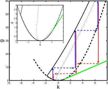
Figure 2: (Color online) Stability boundaries of the single-mode solution of Eq. (21) in the $g$ vs. $k$ plane. Dashed line: neutral stability boundary. Dotted line: stability boundary of the single-mode solution (22) for a continuous spectrum. Solid line: stability boundary of the single-mode solution for $N=92$ and the parameters of Fig. 1. For $k>1$ the bifurcation from zero displacement becomes subcritical and the lower stability boundary is the locus of saddle-node bifurcations (green line). Vertical and horizontal arrows mark the secondary instability transitions shown in Fig. 3.

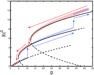
Figure 3: (Color online) A sequence of secondary instabilities following the initial onset of single-mode oscillations in an array of $92$ beams, with the parameters of Fig. 1, plotted as a function of the reduced driving amplitude $g$. Solid (dashed) lines are stable (unstable) solutions defined by (23), for $k=-0.88$, $k^{\prime}=2.81$, and $k^{\prime\prime}=6.51$, corresponding to the first wave number $k$ to emerge and two shifts to $k+\Delta Q_{N}$ and $k+2\Delta Q_{N}$ respectively. Numerical integration of the equations of motion (II) for an upward sweep of $g$ (blue $\times$’s), followed by a downward sweep (red $\circ$’s) exhibits clear hysteresis and confirms the theoretical predictions for the stability of single-mode oscillations as illustrated in Fig. 2.

A transition from one single-mode state to a new single-mode state with a wave number shift of $n\Delta Q_{N}$, for some integer $n$, occurs once the driving amplitude is increased and has crossed the upper bound of the stability balloon. Since the upper bound monotonically increases with $k$, the new wave number will always be larger. A sequence of three transitions, obtained numerically, is shown in Fig. 3, superimposed with our theoretical predictions. The sequence of transitions is also sketched for comparison within the stability balloon in Fig. 2. This type of analysis yields predictions for hysteretic transitions on slow sweeps, with results for when the transition occurs and for the new state that develops, which for larger $g$ must be selected out of a band of possible stable states. It is clear that secondary instabilities allow an additional scenario for observing subcritical transitions, even in very large systems, where the wavenumber separation is small. Once a secondary transition has occurred, the system will return to oscillate in the original wavenumber only when reducing the driving amplitude below the saddle node point of the subcritical bifurcation.

VII Conclusions

We derived amplitude equations (4) describing the response of large arrays of nonlinear coupled oscillators to parametric excitation, directly from the equations of motion yielding exact expressions for all the coefficients. The dynamics at the onset of oscillations was studied by reducing these two coupled equations into a single scaled equation governed by a single control parameter (21). Single mode standing waves were found to be the initial states that develop just above threshold, typical of parametric excitation. The single mode oscillations bifurcate from the zero-displacement state either supercritically or subcritically, depending on the wave number of the oscillations. The wave number dependence originates from the nonlinear gradient terms of the amplitude equation, which were usually disregarded in the past by others in the analysis of parametric oscillations above threshold. We also examined the stability of single mode oscillations, predicting a transition of the initial standing wave state to a new standing wave with a larger wave number as the driving amplitude is increased.

In this work we showed that interesting response of coupled nonlinear oscillators excited parametrically can also be obtained for quasistatic driving amplitude sweeps, rather than the frequency sweeps that are usually preformed in experiments. We proposed, and numerically demonstrated, two experimental schemes for observing our predictions, hoping to draw more experimental attention to the dynamics produced by such sweeps of the driving amplitude.

The results obtained by the numerical integration of the equations of motion agree with our analysis, supporting the validity of the amplitude equation (21). We therefore believe that the amplitude equations we derived can serve as a good starting point for studying other possible states of the system. One particular interesting dynamical behavior that can be considered is that of localized modes, often observed in arrays of coupled nonlinear oscillators and in other nonlinear systems as well. The conditions for obtaining such modes and their dynamical properties could be studied by looking for localized states of the amplitude equations. Another interesting aspect that can be addressed using the amplitude equations we derived is the response of the array to fast (rather than quasistatic) sweeps of the driving amplitude, which should lead to more complicated nonlinear response as observed by LC in their work.