Dynamics of Domain Wall in a Biaxial Ferromagnet With Spin-torque

Abstract

The dynamics of the domain wall (DW) in a biaxial ferromagnet interacting with a spin-polarized current are described by sine-gordon (SG) equation coupled with Gilbert damping term in this paper. Within our frame-work of this model, we obtain a threshold of the current in the motion of a single DW with the perturbation theory on kink soliton solution to the corresponding ferromagnetic system, and the threshold is shown to be dependent on the Gilbert damping term. Also, the motion properties of the DW are discussed for the zero- and nonzero-damping cases, which shows that our theory to describe the dynamics of the DW are self-consistent.

PACS numbers: 75.75.+a, 72.25.Ba, 75.30.Ds, 75.60.Ch

During the past decade or so, rapid advances have been witnessed in both theoretical and experimental aspects toward probing the novel mechanism of spin transfer torque, especially focused on the motion of the domain wall (DW) induced by the spin-polarized current.

Current-driven motion of a DW was studied in a series works by Slonczewski 1 and Berger 2 ; 3 ; 4 . In particular, the phenomenon that the electric current exerts a force on the DW via the exchange coupling was argued in 1984 2 , and a spin-polarized current exerts a torque on the wall magnetization and also the motion due to the pulsed spin-polarized current are studied in 1992 3 , etc.. In the following years these interesting phenomena was observed by many experiments5 ; 6 ; 7 . At the same time there are many theoretical efforts th1 ; th2 ; th3 ; th4 ; th5 ; th6 to understand the microscopic origins. The theoretical works, however, still seem not satisfactorily to explain these phenomena and the intrinsical reason is still unclearly. On the other hand, all experiments 5 ; 6 ; 7 indicate a threshold for the spin-current which induces the motion of the DW, i.e. the motion doesn’t happen until the spin-current strength is lager than the value of this threshold. So, a central theory of the induced domain-wall-motion is to make clear the essential of the threshold, which we proceed to study in this paper.

Very recently, the single-domain-wall as well as its dynamical properties has been observed directly 8 , and another important phenomenon that current inducing a single DW switching exists in ferromagnetic semiconductor has also been demonstrated in experiment 9 . All these experiments offer more information for us to further understand it. At the same time, many discussions have been presented in the refs 10 ; 11 ; 12 ; 13 , especially the kind of spin-torque

$$\tau=-b_{J}\frac{\partial\mathbf{M}}{\partial x},\ \ \ \ b_{J}=\frac{\mu_{B}Pj_{e}}{eM_{s}}$$ (1)

was proposed firstly in 10 and discussed in detail in the refs. 11 ; 12 , where $\mathbf{M}$ is the ferromagnetic magnetization, $M_{s}$ is the saturation magnetization, $P$ is the spin polarization of the current, $\mu_{B}$ is the Bohr magneton and $j_{e}$ is the electric current density. In this paper, considering the above type of spin torque, we study the dynamical properties of the DW in biaxial ferromagnet interacting with a spin-polarized current, focusing on the threshold of the current in the motion of the DW. The threshold is found to be dependent on the Gilbert damping term from the stability condition of the DW’s static state, and the motion of the DW is shown to be a conclusion with the minimal energy of the system.

Now, let us consider a spin-polarized current propagating in a biaxial ferromagnetic material which has an easy x axis and a hard z axis. Here we take an example of a Neel wall and treat the spin configuration as uniform in y-z plane 13 . We assume that the length of magnetization $|\mathbf{M}|$ is constant and the conducting electrons only interact with the local magnetization. In this case, the modified Landau-Lifschitz equation reads

$$\frac{\partial\mathbf{M}}{\partial t}=-\gamma\mathbf{M}\times\mathbf{H}_{eff}+\frac{\alpha}{M_{s}}\mathbf{M}\times\frac{\partial\mathbf{M}}{\partial t}+\tau$$ (2)

where $\gamma$ is the gyromagnetic ratio,

$$\mathbf{H}_{eff}=\frac{2A}{M_{s}^{2}}\nabla^{2}\mathbf{M}+\frac{HM_{x}}{M_{s}}e_{x}-\frac{(H_{\bot}+4\pi M_{s})M_{z}}{M_{s}}e_{z}$$

is effective magnetic field which includes the exchange field, anisotropy field and demagnetization field (note that there exists no external field when the current propagates in the ferromagnet, see, e.g. 8 ; 9 ), H and $H_{\bot}$ are anisotropy fields which correspond to easy axis x and hard axis z respectively, and $\alpha$ is the Gilbert damping parameter. The spin-torque $\tau$ given by Eq. (1) only exists when the ferromagnet has a DW structure such as a microfabricated magnetic wire. The major object in present work is to study the threshold and the dynamics of the DW with Eq. (2). To facilitate the further discussion, we derive the above equation with spherical coordinates $(\theta,\phi)$. By a straightforward calculation, we reach the following equations of $\theta$ and $\phi$

$${\left(\begin{array}[]{lc}\sin\theta&-\alpha\\ \alpha\sin\theta&1\end{array}\right)}{\dot{\phi}\choose\dot{\theta}}={V_{\phi}\choose V_{\theta}}$$ (5)

where

$$V_{\phi} = -\frac{2A\gamma}{M_{s}}(\frac{\partial^{2}\theta}{\partial x^{2}}-sin\theta cos\theta(\frac{\partial\phi}{\partial x})^{2})-\gamma Hsin\theta cos\theta sin\phi cos\phi$$

$$-\gamma(H_{\bot}+4\pi M_{s})sin\theta cos\theta-b_{J}sin\theta\frac{\partial\phi}{\partial x}$$

and

$$V_{\theta}=\frac{2A\gamma}{M_{s}}(sin\theta\frac{\partial^{2}\phi}{\partial x^{2}}+2cos\theta\frac{\partial\theta}{\partial x}\frac{\partial\phi}{\partial x})-\gamma Hsin\theta sin\phi cos\phi-b_{J}\frac{\partial\theta}{\partial x}$$

For convenience we note $H_{\bot}+4\pi M_{s}$ as $H_{\bot}$ in the following derivation. To obtain the threshold, we firstly calculate the static solution to the Eq. (5) and then examine its stability condition with perturbation theory. This is similar to the method used in the ref. 10 . But here, the magnetization $\mathbf{M}$ is a function of the space.

For the biaxial ferromagnet, one has $H_{\bot}\gg H,\sin\theta\simeq 1$ and $\cos\theta\simeq 0$ integ . Thus the static solution is governed by $V_{\phi}=V_{\theta}=0$, i.e.

$$b_{J}\frac{\partial\phi}{\partial x}+\gamma\cos\theta H_{\bot}=0,$$ (6)

$$(\frac{2A\gamma}{M_{s}}-\frac{b_{J}^{2}}{\gamma H_{\bot}})\frac{\partial^{2}\phi}{\partial x^{2}}-\gamma H\sin\phi\cos\phi=0.$$ (7)

With the boundary condition $\phi(-\infty)=0$ and $\phi(\infty)=\pi$, one finds the form of the static kink soliton perturbation reads: $\phi=2\arctan[\exp(\pm\frac{x}{\xi})]$, where these solutions are referred to head-to-head DW (+ sign) and tail-to-tail DW (- sign) 8 and $\xi=\sqrt{\frac{2A}{MH}-\frac{b_{J}^{2}}{\gamma^{2}HH_{\bot}}}$ indicates that the spatial width of the soliton becomes narrower when the current strength increases (Fig.1).

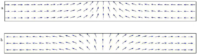
Figure 1: (a) head-to-head DW, result of $\phi$=$2\arctan[\exp(\frac{x}{\xi})]$. (b) tail-to-tail DW, result of $\phi$=$2\arctan[\exp(-\frac{x}{\xi})]$.

In the following part, we consider the head-to-head DW and proceed to calculate the threshold with perturbation theory. (This theory can also be used in a tail-to-tail DW and gets the same result.) For this we allow the static soliton solution develop a small dynamic factor, i.e. $\phi\rightarrow\phi^{\prime}$:

$$\phi^{\prime}=2\arctan[\exp((1+a(t))\frac{x}{\xi}+b(t))]$$ (8)

where $b(t)$ is a small perturbation and $a(t)$ is a higher order smallness of $b(t)$ with $a(t)\sim(\frac{\partial b(t)}{\partial t})^{2}$(This can be derived from the dynamic solution of SG equation). Then, one has $\delta\phi=\phi^{\prime}-\phi=\frac{\partial\phi}{\partial x}b(t)$ and the equations of $\delta\phi$, $\delta\theta$ can be written as

$$\frac{\partial}{\partial t}{\delta\phi\choose\delta\theta}=\frac{1}{1+\alpha^{2}}{\left(\begin{array}[]{lc}-b_{J}\frac{\phi_{xx}}{\phi_{x}}&\gamma H_{\bot}\\ \alpha b_{J}\frac{\phi_{xx}}{\phi_{x}}&-\alpha\gamma H_{\bot}\end{array}\right)}{\delta\phi\choose\delta\theta}=\frac{1}{1+\alpha^{2}}\hat{D}{\delta\phi\choose\delta\theta}$$ (11)

One can verify that the eigenvalues $\lambda$ of the matrix $D$ is given by

$$\lambda_{1}=0,\ \ \ \ \ \ \ \ \ \ \ \lambda_{2}=\frac{b_{J}}{\xi}\tanh(\frac{x}{\xi})-\alpha\gamma H_{\bot}$$

It is obvious that the stability condition of the solution $\phi$ depends on the properties of the eigenvalues stable . Since $\lambda_{1}$=0, the static solution can be steady only if $\lambda_{2}\leq 0$ at any position. For this one finds a critical value for the current

$$J^{cr}_{e}=\frac{\alpha\gamma H_{\bot}e}{P\mu_{B}}\sqrt{\frac{2A}{M_{s}H(1+\frac{\alpha^{2}H_{\bot}}{H})}}$$ (12)

above which the static DW can not be stable any more, i.e. $J^{cr}_{e}$ is the threshold of the current. Since the value of the function $\tanh x$ keeps approximate 1 from $x\rightarrow\infty$ to the edge of the DW (we calculate this value with matlab, e.g. when $x=2\xi$, one gets $\tanh(2)=0.9640$), the DW becomes unstable firstly at its edge. The pinning force 13 is not considered in our derivation, thus not the pinning force, but the Gilbert damping term $\alpha$ is the exclusive factor for existing a threshold in our argument. Furthermore, if $\frac{\alpha^{2}H_{\bot}}{H}\ll 1$ (Because $\alpha$ may be very small, it’s not contrary with the assumption that $H_{\bot}\gg H$), one finds the threshold is proportional to the $H_{\bot}$ and the wall-parameter $\sqrt{\frac{2A}{M_{s}H}}$ as well 13 .

Now, we proceed to reveal properties of the motion for the DW above the threshold. Also, we begin with Eq. (2). For the case $H_{\bot}\gg H$, $\sin\theta\approx 1$ and $cos\theta\approx 0$, the dynamic equation takes the following coupled form

$$\sin\theta\frac{\partial\phi}{\partial t}-\alpha\frac{\partial\theta}{\partial t}=-b_{J}\frac{\partial\phi}{\partial x}-\gamma cos\theta H_{\bot}$$ (13)

$$\alpha sin\theta\frac{\partial\phi}{\partial t}+\frac{\partial\theta}{\partial t}=\frac{2A\gamma}{M_{s}}\frac{\partial^{2}\phi}{\partial x^{2}}-\gamma Hsin\phi cos\phi-b_{J}\frac{\partial\theta}{\partial x}$$ (14)

As the method used in 12 , we differentiate equation (13) and substitute it into Eq. (14) yields

$$\frac{\partial^{2}\phi}{\partial t^{2}}-(\frac{2A\gamma^{2}H_{\bot}}{M_{s}}-b_{J}^{2})\frac{\partial^{2}\phi}{\partial x^{2}}+2b_{J}\frac{\partial^{2}\phi}{\partial x\partial t}+\gamma^{2}HH_{\bot}sin\phi cos\phi+\alpha\gamma H_{\bot}\frac{\partial\phi}{\partial t}=0$$ (15)

From above formula one finds an additional term $2b_{J}\phi_{xt}$ (the third term of the left side) of Eq. (15) is added due to the spin current. To facilitate the further discussions, we make transformations: $t^{{}^{\prime}}=tcos\beta+\kappa xsin\beta,\ \ x^{{}^{\prime}}=-tsin\beta+\kappa xcos\beta,\ \tan 2\beta=b_{J}\kappa$, where $\kappa=1/\sqrt{\frac{2A\gamma^{2}H_{\bot}}{M_{s}}-b_{J}^{2}}=\sqrt{\frac{M_{s}}{2A\gamma^{2}H_{\bot}}}\zeta$ with $\zeta>1$. Using these new coordinates, the Eq. (15) recasts into

$$\frac{1}{\cos 2\beta}(\frac{\partial^{2}\psi}{\partial t^{{}^{\prime}2}}-\frac{\partial^{2}\psi}{\partial x^{{}^{\prime}2}})+\gamma^{2}HH_{\bot}sin\psi+\alpha\gamma H_{\bot}(cos\beta\frac{\partial\psi}{\partial t^{{}^{\prime}}}-sin\beta\frac{\partial\psi}{\partial x^{{}^{\prime}}})=0$$ (16)

where $\psi=2\phi$. To give a more intuitive discussion, we neglect the damping term in the following derivation. Then, under the boundary condition: $\psi(-\infty)=0\ \ \psi(\infty)=2\pi$, we obtain kink soliton solution of the Eq. (15):

$$\phi = 2arctan[\exp(\sqrt{\frac{\gamma^{2}HH_{\bot}\cos 2\beta}{(1-v^{2})}}(x^{{}^{\prime}}-vt^{{}^{\prime}}))]$$ (17)

$$=2arctan[\exp(\sqrt{\frac{\gamma^{2}HH_{\bot}\cos 2\beta}{(1-v^{2})}}(\kappa x(\cos\beta-v\sin\beta)-t(\sin\beta+v\cos\beta)))]$$

where $v$ is the velocity of the DW in $x^{{}^{\prime}}-t^{{}^{\prime}}$ coordinate and a free parameter subject only to the restriction $|v|\leq 1$, and it is related to the velocity $\mathbf{V}$ by $\mathbf{V}$=$\frac{v\cos\beta+\sin\beta}{\kappa(\cos\beta-v\sin\beta)}$. With this solution we can calculate the energy of the DW for the motion case. Deriving from the Lagrangian $L=\int d^{3}x(M_{s}\dot{\phi}(\cos\theta-1)-E)$, one can obtain the hamiltonian in the following form:

$$H=\int d^{3}xE=\int d^{3}x(2A((\nabla\theta)^{2}+\sin\theta(\nabla\phi)^{2})-HM_{s}(\sin\theta\cos\phi)^{2}+H_{\bot}M_{s}\cos^{2}\theta).$$ (18)

This result is valid no matter whether the DW is steady or not, and it indicates that there is no kinetic energy in the hamiltonian even for the propagating case of the domain wall. Substituting the Eq. (17) into (18), we obtain the DW energy $E$ as

$$E = 2\sqrt{2AM_{s}H\cos 2\beta}\zeta\{\frac{\cos\beta-v\sin\beta}{\sqrt{1-v^{2}}}+\frac{\sqrt{1-v^{2}}}{\cos 2\beta\zeta^{2}(\cos\beta-v\sin\beta)}+$$ (19)

$$\frac{M_{s}}{\gamma^{2}H_{\bot}2A}\frac{(b_{J}(\cos\beta-v\sin\beta)-(\sin\beta+v\cos\beta)/\kappa)^{2}}{\sqrt{1-v^{2}}(\cos\beta-v\sin\beta)}\}+C$$

where $C$ is a constant independent on any parameters. Eq. (19) tells us that the total energy of the DW is the function of the parameters $v$ and $\beta$. The first term in the bracket of the right side of above equation corresponds to exchange energy, the second term corresponds to the anisotropy energy of the easy axis and the third one corresponds to the anisotropy energy of the hard axis. By a straightforward calculation we find that the total energy E reaches its minimum when $v=\tan\beta$.

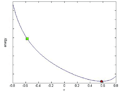
Figure 2: DW energy as a function of parameter $v$($|v|\leq 1$). The velocity of the DW $\mathbf{V}$=$\frac{v\cos\beta+\sin\beta}{\kappa(\cos\beta-v\sin\beta)}$. Green square represents the energy of DW when $\mathbf{V}=0$ and red hexagon represents the minimal energy of DW when $\mathbf{V}=b_{J}$(we take an example of $\beta=\frac{\pi}{6}$).

Therefore in this case, the DW structure can be described as

$$\phi_{min}=2\arctan[\exp(\frac{\cos 2\beta}{\xi}(x-b_{J}t))]$$ (20)

The above formula clearly shows that the distribution of $\phi_{min}$ is similar to the static soliton solution except for a velocity $b_{J}$ and $M_{z}=0$. So, if the damping term $\alpha=0$, the DW moves once the spin current is applied, and the threshold arrives at zero. These results are self-consistent with the former derivation that the threshold is proportional to the damping $\alpha$ (see eq. (12)).

Before sum up, we should point out that practically the velocity observed in experiment will be smaller than $b_{J}$ for the nonzero damping term. For a brief discussion on this effect one may assume the initial velocity of the DW is $b_{J}$ 12 in the above-threshold case. With perturbation theory on the SG soliton, after Lorentz transformation to the soliton’s rest frame $z-\tau$ and noting that $\psi=2\phi$, we obtain a series of equations similar to that in ref. perturbation :

$$\phi(z,\tau)=\phi_{min}(z,\tau)+\xi(z,\tau),$$ (21)

here $\phi_{min}$ (see eq. (20)) is described in $z-\tau$ frame and $|\xi(z,\tau)|\ll 1$ perturbation and

$$\xi(z,\tau)=\frac{1}{8}u_{b}(\tau)f_{b}(z)+\int^{\infty}_{-\infty}dku_{k}(\tau)f_{k}(z),$$ (22)

$$\frac{\partial^{2}\psi}{\partial\tau^{2}}-\frac{\partial^{2}\psi}{\partial z^{2}}+\sin\psi+\nu(\frac{\partial\psi}{\partial\tau}-\tan 2\beta\frac{\partial\psi}{\partial z})=0,$$ (23)

where $f_{b}(z)=2sech(z)$, $f_{k}(z)=(2\pi)^{\frac{1}{2}}\omega_{k}^{-1}[k+i\tanh(z)]\exp(ikz)$, $\omega_{0}^{2}$=$\gamma^{2}HH_{\bot}\cos 2\beta$, $\omega_{k}=1+k^{2}$ and $\nu$=$\frac{\alpha\gamma H_{\bot}\cos^{\frac{3}{2}}2\beta}{\omega_{0}}$. Note that in Eq. (23) $\tan 2\beta$ is not a small value, we approximately obtain the amplitude of the translational mode $u_{b}$ satisfies

$$\frac{du_{b}(\tau)}{d\tau}=(8\tan 2\beta(1-\exp(-\nu\tau))+\exp(-\nu\tau)\int f(\tau)\exp(\nu\tau)d\tau)$$ (24)

with $f(\tau)=i(\pi/2)^{\frac{1}{2}}(\tan 2\beta)\nu\int^{\infty}_{-\infty}dk[ku_{k}(\tau)]/(\omega_{k}\sinh\frac{1}{2}\pi k)$. This formula means that in $z-\tau$ frame, the DW will get a velocity equal to $(-du_{b}/d\tau)$ perturbation . From above result one easily find the velocity of the DW $\mathbf{V}$ should be smaller than $b_{J}$. While we can not let $\tau\sim\infty$ to get the terminal velocity because for large $\tau$, this perturbation theory breaks down since $u_{b}$ grows with $\tau$. In fact, theoretically the motion will not stop as long as the spin current strength is larger than the threshold value, because the damping term will disappear once the velocity becomes zero and then according to present result this static solution is obviously a high energy state, which is not steady.

The development herein is outlined as follows. Initially, no spin current is applied to the biaxial ferromagnet, the variable $\theta=\pi/2$ and the DW can be described as static soliton solution of SG equation. Secondly, a current is applied while the DW still keeps static if the current strength is smaller than the threshold value, and its width becomes short in x-y plane. On the other hand, the magnetization $\mathbf{M}$ develops a component $M_{z}$ as is shown in Eq. (6),

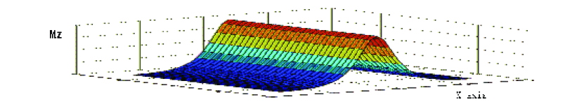
Figure 3: With spin-torque, the out-of-plane component $M_{z}$ as a function of $x$-coordinate, is uniform in y-z plane.

the value of $M_{z}$ and the anisotropy energy of hard axis increase with time due to the increasing current strength till which arrives at the threshold (Fig. 3). Thirdly, for the above-threshold case, the static DW can’t support the increasing of $M_{z}$, i.e. this case will result in the propagation of the DW along the motion direction of the conducting electrons in the current. Then, neglecting the Gilbert damping term, we discuss the dynamical properties of Landau-Lifshitz equation by discovering a series of solutions which respectively correspond to different energies of the DW and find the velocity of the DW induced by the spin-current is $b_{J}$, which corresponds to the minimal energy of the DW. Finally, for the nonzero-damping case, the velocity of the DW is found to be smaller than $b_{J}$. With these derivations we show our result is self-consistent that the threshold depends on the Gilbert damping term of the coupled Landau-Lifschitz equation.

In conclusion the dynamical properties of a single DW is studied in biaxial ferromagnet induced by a torque exerted via the spin-polarized current. With the perturbation theory on the static kink soliton solution to the ferromagnetic system, we obtain a threshold of the current in the motion of domain wall and the threshold is shown to be dependent on the Gilbert damping term of the coupled Landau-Lifschitz equation. Also, the motion properties of the DW are discussed in the zero- and nonzero-damping cases, which shows that our theory to describe the dynamics of the DW are self-consistent.

The authors are grateful to B. S. Han and D. J. Zheng for their wonderful lectures on spintronics in Nankai University. It’s these lectures that lead us to this attractive field. This work is supported by NSF of China under grants No.10275036 and No.10304020.

References

- (1) J.C.Slonczewski, J.Magn.Magn.Mater. 159, L1(1996); 195, L261(1999)
- (2) L.Berger, J. Appl. Phys. 55, 1954 (1984)
- (3) L.Berger, J. Appl. Phys. 71,2721 (1992)
- (4) L.Berger, Phys. Rev. B 54, 9353 (1996)
- (5) M. Tsoi et al., Phys. Rev . Letter, 80, 4281 (1998)
- (6) E.B.Myers,D.C.Ralph,J.A.Katine,R.N.Louie,and R.A.Buhrman, Science 285, 867 (1999)
- (7) J.A.Katine,F.J.Albert,R.A.Buhrman,E.B.Myers,and D.C.Ralph, Phys.Rev.Lett. 84, 3149 (2000)
- (8) M. Tsoi, A.G.M. Jansen, J. Bass, W.-C. Chiang, M. Seck, V. Tsoi, and P. Wyder, Phys. Rev. Lett. 80, 4281 (1998)
- (9) E.B. Myers, D.C. Ralph, J.A. Katine, R.N. Louie, and R.A. Buhrman, Science 285, 867 (1999)
- (10) J.Z. Sun, J. Magn. Magn. Mater. 202, 157 (1999)
- (11) J.A. Katine, F.J. Albert, R.A. Buhrman, E.B. Myers, and D.C. Ralph, Phys. Rev. Lett. 84, 3149 (2000)
- (12) J. Grollier, V. Cros, A. Hamzic, J.M. George, H. Jaffres, A. Fert, G. Faini, J. Ben Youssef, and H. Legall, Appl. Phys. Lett. 78, 3663 (2001); F.J. Albert, J.A. Katine, R.A. Buhrman, and D.C. Ralph, Appl. Phys. Lett. 81, 2202 (2002)
- (13) S. Zhang, P. M. Levy, A. Fert, Phys. Rev. Lett. 88, 236601 (2002); Z. Li and S. Zhang, Phys. Rev. B. 68, 024404 (2003)
- (14) A.Yamaguchi et.al., Phys.Rev.Lett. 92, 077205 (2004)
- (15) M.Yamanouchi,D.Chiba,F.Matsukura and H.Ohno., Nature 428, 539 (2004)
- (16) Ya.B.Bazaliy,B.A.Jones,and S.-C.Zhang., Phys.Rev.B. 57, R3213 (1998)
- (17) Zai-Dong Li,J.-Q.Liang,Lu.Li,and W.-M Liu, Phys.Rev.E. 69, 066611 (2004)
- (18) Z.Li and S.Zhang, Phys.Rev.Lett. 92, 207203 (2004); Z.Li and S.Zhang, Phys. Rev. B 70, 024417 (2004)
- (19) Gen. Tatara and Hiroshi. Kohno, Phys.Rev.Lett. 92 086601 (2004)
- (20) Ya.B.Bazaliy,B.A.Jones,and S.-C.Zhang.,Phys.Rev.B, 69, 094421 (2004)
- (21) M. B. Fogel, S. E. Trullinger, A. R. Bishop, and J. A. Krumhansl, Phys. Rev. B 15,1578 (1977); H. How, R. C. O’Handley, and F. R. Morgenthaler, Phys. Rev. B 40, 4808 (1989)
- (22) Y. S. Kivshar and B. A. Malomed, Reviews of Modern Physics, 61,763 (1999)