Effective one-component description of two-component Bose-Einstein condensate dynamics

Abstract

We investigate dynamics in two-component Bose-Einstein condensates in the context of coupled Gross-Pitaevskii equations and derive results for the evolution of the total density fluctuations. Using these results, we show how, in many cases of interest, the dynamics can be accurately described with an effective one-component Gross-Pitaevskii equation for one of the components, with the trap and interaction coefficients determined by the relative differences in the scattering lengths. We discuss the model in various regimes, where it predicts breathing excitations, and the formation of vector solitons. An effective nonlinear evolution is predicted for some cases of current experimental interest. We then apply the model to construct quasi-stationary states of two-component condensates.

I Introduction

One of the most intriguing aspects of recently produced atomic Bose-Einstein condensates BEC is the ease with which two (or more) internal levels can be populated, in effect forming a spin-1/2 (or spin-1, etc.) system. In particular, phase separation phaseSepExp ; phaseSepTh , vector solitons twoCompSolitonsBEC , two-component vortices twoCompVortex ; twoCompVortexLatt ; vortexStorage ; twoCompVortexStab , spin waves spinWaves , breathe-together solutions dynamics ; breatheTogether and more general issues regarding the dynamics multipleComponentJILA ; symBreaking ; dynamics and stability twoCompStab in these systems have recently been investigated. Two-component BECs hold promise for a number of applications, including coherent storage and processing of optical fields processing using stopped light techniques stoppedLight .

The dynamics of two-component BECs is in general a difficult problem to study analytically, and much of the recent activity has focused on particular situations and thus made specific assumptions. For example, the relative interaction strengths (via the binary collision scattering lengths) for inter- and intra-component collisions are sometimes presumed to be equal, whereas in practice these scattering lengths vary and depend on the atom and the particular levels utilized. Furthermore, these can be experimentally varied with Feshbach resonances feshbach . In other studies it is assumed there is little or no spatial variation in the relative density between the two components, restricting the applicability of these calculations to many cases of interest. For example, in stopped light experiments, a highly spatially dependent superposition of the two internal atomic states are generated by light pulses, and the dynamics of this inhomogenous superposition is essential in determining the information storage and processing capabilities of the system processing .

The need for a simple understanding of dynamics in two-component BECs free of such assumptions is the motivation for this work. We specifically consider the experimentally relevant situation of a single-component BEC (in an internal state labelled $|1\rangle$) in its ground state, whose constituent atoms are suddenly put into spatially dependent superposition of two internal levels ($|1\rangle$ and $|2\rangle$), with the $|2\rangle$ condensate occupying a region inside the larger $|1\rangle$ condensate. Such a situation occurs with stopped light pulses processing or spatially dependent Raman pulses. When such processes occur fast compared to the atomic dynamics (millisecond timescales), the resulting two-component BEC will initially have the same density profile as the original single-component BEC. However, this is not a stationary state and will evolve. The evolution can be modelled with coupled Gross-Pitaevskii (GP) equations, where each component is described with a single macroscopic wave functions $\psi_{1}$ and $\psi_{2}$.

We find, remarkably, that the evolution of $\psi_{2}$ can often be described with an effective single-component GP equation, with the trapping potential and interaction coefficients renormalized by the fractional difference in scattering lengths. Those these differences are generally small in practice, they end up dominating the motion of the wave functions. Depending on their sign and magnitude, our model predicts both trapping and repulsive effective potentials, as well as positive (repelling) or negative (attractive) effective scattering lengths for the $|2\rangle$ condensate.

The reduction to a single-component picture is accomplished by observing that the fluctuations of the total density are smaller and more quickly varying than the evolution of each individual component. We find an equation of motion for the total density fluctuations and find that, within certain limits, these fluctuations are described with a simple expression which we can plug into the equation of motion for $\psi_{2}$ and derive our effective one-component description. While we will perform our calculations with one-dimensional equations for computational simplicity, the results are equally valid and applicable in full three-dimensional geometries.

Using our model, much of the vast existing literature on single-component BEC dynamics can be easily be applied to predict analogous behavior in two-component systems. To demonstrate this applicability, and test the accuracy of our model, we present calculations in several parameter regimes. For certain relative scattering lengths we get a repulsive effective nonlinearity in a trap. In this case a simple breathing motion occurs and the existing analytic results on collective excitations in single-component BECs oneCompExcitations can be applied. In other cases, we get an attractive nonlinearity, in which case phase separation occurs and vector solitons form and propagate. Our model again allows a mapping onto existing literature on the formation of soliton trains in single component BECs solitonTrainExp ; solitonTrainTh which should improve abilities to design and analyze experiments to observe vector solitons, which have hitherto not been ovserved. We also note that the levels $|F=1,M_{F}=-1\rangle$ and $|F=2,M_{F}=+1\rangle$ in ⁸⁷Rb, used in many present day experiments multipleComponentJILA ; twoCompVortex , give rise to a vanishing effective nonlinearity, allowing us predict the evolution with a linear Schroedinger equation. This should prove especially powerful in two and three dimensional cases, where it is computationally expensive to solve the full nonlinear differential equations. Finally, we use our model to predict the existence of solutions whereby two overlapping condensates (each with arbitrary number) remain nearly stationary for very long times. These solutions can be thought of as generalizing previously discussed breathe-together solutions dynamics ; breatheTogether . These solutions are relevant to observing spin squeezing spinSqueezing and coherent optical storage processing in these systems.

II Derivation of the one-component model

II.1 Description of the system

The coupled GP equations governing the evolution are

$$i\hbar\frac{\partial\psi_{1}}{\partial t} = \bigg{[}-\frac{\hbar^{2}}{2m}\frac{\partial^{2}}{\partial z^{2}}$$ (1)

$$+V(z)+U_{11}|\psi_{1}|^{2}+U_{12}|\psi_{2}|^{2}\bigg{]}\psi_{1}$$

$$i\hbar\frac{\partial\psi_{2}}{\partial t} = \bigg{[}-\frac{\hbar^{2}}{2m}\frac{\partial^{2}}{\partial z^{2}}$$ (2)

$$+V(z)+U_{22}|\psi_{2}|^{2}+U_{12}|\psi_{1}|^{2}\bigg{]}\psi_{2},$$

where $m$ is the mass of the atoms and the harmonic external trapping potential $V(z)=\frac{1}{2}m{\omega_{z}}^{2}z^{2}$ is assumed to be equal for each component (which is true in particular sub-levels for magnetic traps multipleComponentJILA for and for all sub-levels in far off-resonant optical traps opticalTrap ). Atom-atom interactions are characterized by the $U_{ij}=4\pi N\hbar^{2}a_{ij}/mA$, where $N$ is the total number of condensate atoms, $a_{ij}$ are the s-wave scattering lengths for binary collisions and between atoms in internal states $|i\rangle$ and $|j\rangle$. We are only accounting for dynamics in the the $z$ dimension, which is valid in an elongated trap geometry where the significant dynamics occur primarily in this dimension sound , and so choose an effective transverse area $A$ to give the correct nonlinearity . We will show how the relative difference in the scattering lengths are key parameters in the evolution and so define $\delta_{c}\equiv(a_{12}-a_{11})/a_{11}$ and $\delta_{2}\equiv(a_{22}-a_{11})/a_{11}$.

For concreteness, we consider a condensate with $N=2.0\times 10^{6}$ atoms in a trap with frequency $\omega_{z}=(2\pi)~{}21~{}\mathrm{Hz}$. The area $A=\pi(4.2~{}\mu\mathrm{m})^{2}$ is chosen such that the initial density in the center corresponds to a ground state BEC in a cylindrically symmetric trap with a transverse frequency $\omega_{r}=8\omega_{z}$. The density profile of this initial state, labelled $\rho_{0}$, is plotted as the dotted curve in the first panel of Fig. 1(a). We then assume the BEC is put into a spatial superposition of two states with a Gaussian-shaped and slightly off-center wavefunction $\psi_{2}$, inside the larger $|1\rangle$ condensate [again see the first panel of Fig. 1(a)]. The total density still given by $\rho_{0}$ but, because of the spin excitation, this is no longer a stationary state.

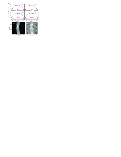
Figure 1: (a) The densities $N|\psi_{2}|^{2}$ (solid curve, red online) and $N|\psi_{1}|^{2}$ (dashed curve, blue online), and total density $N\rho$ (dotted, black curve) at the times indicated. The initial total density $\rho_{0}$ corresponds to the ground state of a pure $|1\rangle$ condensate. The dot-dashed curve shows the fluctuations of the total density $\delta\rho$ scaled by $-1/\delta_{c}$. (b) The time evolution of the density profile $|\psi_{2}|^{2}$ in this case. (c) The time evolution of $\delta\rho$.

The resulting two-component evolution is presented in Fig. 1(a). Here we have chosen $\delta_{2}=-0.03$ and $\delta_{c}=-0.03$. As we observe in the figure, each component undergoes non-trivial evolution of its density profile while the overall density profile (which we define to be $\rho\equiv|\psi_{1}|^{2}+|\psi_{2}|^{2}$) undergoes only very small fluctuations. To get a sense of the shape and magnitude of these small fluctuations, the dot-dashed curves show the deviations from the original density profile, $\delta\rho\equiv\rho-\rho_{0}$, blown up by the factor $-1/\delta_{c}\approx 33$ (the reason for this particular case will become apparent later). One sees that at 15 ms a slight fluctuation in the total density has appeared in the region occupied by $|2\rangle$ as well as near the condensate edges (in such a way that the total atom number is conserved). Figure 1(b) gives an overview of the evolution of the density profile $|\psi_{2}|^{2}$ and one sees that there is a breathing like behavior, with the width becoming larger and then smaller, as well as a small dipole sloshing due to its original offset from the trap center. Figure 1(c) then shows the evolution of the density fluctuations $\delta\rho$ and one observes two important features. First there is a pair of density perturbations travelling back and forth across the $|1\rangle$ BEC (and reflecting at its boundaries), which, as we will see below, are travelling at the sound speed determined by the total BEC density. In the panels of Fig. 1(a), showing 15 ms and 45 ms, these waves are near the BEC boundary whereas at 30 ms they are crossing in the region occupied by $|\psi_{2}|^{2}$. Second, there is a part which appears to be closely mimicking the much more slowly evolving profile of $|\psi_{2}|^{2}$ (as also seen in the Fig. 1(a) plots).

II.2 Calculation of density fluctuations

We now analytically investigate the coupled GP equations (1-2) to learn how this particular pattern for the total density fluctuations arises. Our strategy will be to eliminate the wavefunction $\psi_{1}$ in favor of a hydrodynamic description of the total density $\rho$ and total velocity field $v_{c}=(v_{1}|\psi_{1}|^{2}+v_{2}|\psi_{2}|^{2})/\rho$, where $v_{i}=(\hbar/m)\phi_{i}^{\prime}$ are the velocity fields of each component (the $\phi_{i}^{\prime}$ denote the gradients of the phases of the wavefunctions $\psi_{i}$; we will use the prime symbol to indicate $\partial/\partial z$). We then linearize in the small density fluctuations $\delta\rho$ and consequently small velocity field $v_{c}$. Our observation that $\delta\rho$ evolves on a fast time scale relative to $\psi_{2}$ supplies an obvious separation of time scales in the problem and allows us to then solve for the evolution $\delta\rho$ assuming $\psi_{2}$ is static on this time scale.

For convenience we define the relative density in $|2\rangle$ to be $f=|\psi_{2}|^{2}/\rho$, so $1-f=|\psi_{1}|^{2}/\rho$. After some lengthy, but straightforward, algebra one can show that Eqs. (1-2) imply

$$\dot{\rho} = -\rho v_{c}^{\prime}-\rho^{\prime}v_{c},$$ (3)

$$\dot{v_{c}} = -\frac{1}{m}\big{[}V^{\prime}(z)+U_{11}\rho^{\prime}+\epsilon_{MF}^{\prime}$$ (4)

$$+\epsilon_{KE}^{\prime}+\epsilon_{SP}^{\prime}+\epsilon_{QP}^{\prime}\big{]};$$

$$\mathrm{where}$$

$$\epsilon_{MF1}^{\prime} = U_{11}\rho\big{[}\delta_{2}ff^{\prime}+\delta_{c}f^{\prime}(1-2f)\big{]},$$ (5)

$$\epsilon_{MF2}^{\prime} = U_{11}\rho^{\prime}\big{[}1+\delta_{2}f^{2}+2\delta_{c}f(1-f)\big{]},$$ (6)

$$\epsilon_{KE}^{\prime} = (1-f)\bigg{[}\frac{1}{2}mv_{1}^{2}\bigg{]}^{\prime}+f\bigg{[}\frac{1}{2}mv_{2}^{2}\bigg{]}^{\prime}$$ (7)

$$+f(1-f)\frac{\rho^{\prime}}{\rho}\bigg{[}\frac{1}{2}m(v_{1}-v_{2})^{2}\bigg{]}$$

$$+f(1-f)\bigg{[}\frac{1}{2}m(v_{1}-v_{2})^{2}\bigg{]}^{\prime}$$

$$-\frac{1}{2}m(v_{1}-v_{2})f^{\prime}\big{[}fv_{1}+(1-f)v_{2}\big{]},$$

$$\epsilon_{SP}^{\prime} = \frac{\hbar^{2}}{4m}\bigg{[}\frac{f^{\prime 2}}{f(1-f)}\bigg{]}^{\prime}+\frac{\hbar^{2}}{4m}\frac{\rho^{\prime}}{\rho}\bigg{[}\frac{f^{\prime 2}}{f(1-f)}\bigg{]},$$

$$\epsilon_{QP}^{\prime} = \frac{\hbar^{2}}{8m}\bigg{[}\frac{\rho^{\prime 2}}{\rho^{2}}-2\frac{\rho^{\prime\prime}}{\rho}\bigg{]}.$$ (8)

We next linearize in the velocity field $v_{c}$ and density fluctuations $\delta\rho=\rho-\rho_{0}$. In this context, $\rho_{0}$ is defined as the single component ($f=0$) stationary solution:

$$V+U_{11}\rho_{0}+\frac{\hbar^{2}}{8m}\frac{(\rho_{0}^{\prime 2}-2\rho_{0}\rho_{0}^{\prime\prime})}{\rho_{0}^{2}}=0.$$ (9)

Performing the linearization and eliminating $v_{c}$ yields a second order equation for the density fluctuations:

$$\ddot{\delta\rho} = \frac{\rho_{0}}{m}\bigg{[}U_{11}\delta\rho^{\prime}+\epsilon_{MF1}^{(1)^{\prime}}+\epsilon_{MF2}^{(1)^{\prime}}+\epsilon_{KE}^{(1)^{\prime}}+\epsilon_{SP}^{(1)^{\prime}}\bigg{]}^{\prime}$$ (10)

$$\frac{\rho_{0}^{\prime}}{m}\bigg{[}U_{11}\delta\rho^{\prime}+\epsilon_{MF1}^{(1)^{\prime}}+\epsilon_{MF2}^{(1)^{\prime}}+\epsilon_{KE}^{(1)^{\prime}}+\epsilon_{SP}^{(1)^{\prime}}\bigg{]}$$

where $\epsilon_{MF1}^{(1)^{\prime}},\epsilon_{MF2}^{(1)^{\prime}},\epsilon_{KE}^{(1)^{\prime}},$ and $\epsilon_{SP}^{(1)^{\prime}}$ and are obtained by making the replacement $\rho\rightarrow\rho_{0}$ in the corresponding expressions (5-II.2). In this expression we have dropped terms involving the product of the fluctuations $\delta\rho$ with kinetic energy terms and relative scattering length differences $\sim\delta_{c},\delta_{2}$.

Equation (10) is quite widely applicable, however it turns out that in practice we can simplify things further; in the Thomas-Fermi regime the spatial derivatives of the background density $\rho_{0}$ are small compared to the mean field and as a result the second line of Eq. (10) can be neglected relative to the first line. The result is an intuitively simple picture: The first term implies the density fluctuations obey a phonon-like dispersion term with usual sound speed in the condensate $c_{0}\equiv\sqrt{U_{11}\rho_{0}/m}$, while the remaining terms of the first line provide various source terms which seed these density fluctuations and are non-zero only in locations where there is a spin-excitation (that is, where $f\not=0$). These source terms occur both because of differences in the mean field interaction between the components as well as kinetic energy and quantum pressure in the two wavefunctions. Because the spin dynamics are much slower than the sound speed propagation, the source terms appear to be nearly stationary to the phonons.

Armed with this picture, we can now interpret Fig. 1(c). The initial spin excitation gives non-zero source terms that generate phonons, which then propagate through the BEC towards the boundary. Meanwhile, in the region of the spin excitation, the fluctuations are driven into a quasi-steady state solution. In an infinite medium the phonons would continue, however here they reflect off the boundaries and so repeatedly cross the area of the spin excitation. In the Fig. 1, such a crossing occurs at 30 ms, while reflections off the boundaries occur at 15 ms and 45 ms.

In many cases of interest, the mean field contribution $\epsilon_{MF1}^{(1)^{\prime}}$ dominates the kinetic energy contributions in Eq. (10). In this case it is easy to solve for the quasi-steady state solution $\delta\rho^{\mathrm{(ss)}}$ by setting $\ddot{\delta\rho}=0$:

$$\delta\rho^{\mathrm{(ss)}} = -\rho_{0}\bigg{[}\delta_{c}f+\frac{1}{2}f^{2}(\delta_{2}-2\delta_{c})\bigg{]}$$ (11)

When $f\ll 1$ this reduces to $\delta\rho^{\mathrm{(ss)}}=-\delta_{c}|\psi_{2}|^{2}$, which predicts fluctuations which are directly proportional to the density in $|2\rangle$. This approximate solution holds fairly well in the example, as shown by the dot-dashed curves in Fig. 1(a). At 15 ms and 45 ms the sound waves are primarily at the BEC edge and this quasi-steady state solution dominates in the area of the spin-excitation. At 30 ms, the sound waves are passing through the spin excitation region and are comparable to the quasi-steady state part. These sound waves end up having virtually no impact on the evolution of $\psi_{2}$ due to the fact that their evolution is on a completely different and independent time scale. Stated another way, though the sound waves overlap $\psi_{2}$ each time they cross the BEC, the contributions from each crossing tend to be out of phase and their net contribution to the evolution of $\psi_{2}$ washes out to nearly zero. On the other hand the quasi-steady state part, given by Eq. (11), can have a large impact on the evolution of $\psi_{2}$.

Explicit numerical calculation of the various source terms reveals that the mean field term indeed dominates by more than an order of magnitude, meaning Eq. (11) should hold. Furthermore, inspection of the figure shows that the initial peak relative density is $f\sim 1/5$ and the first term should dominate.

II.3 Effective one-component GP equation

The existence of this simple solution allows us to then solve for the much slower evolution of $\psi_{2}$. Re-writing (2) in terms of $\delta_{c},\delta_{2}$, eliminating $|\psi_{1}|^{2}$ in favor of $\rho$ and using our solution of (9) for the initial density profile $\rho_{0}$ allows us to write:

$$i\hbar\frac{\partial\psi_{2}}{\partial t} = \bigg{[}\frac{-\hbar^{2}}{2m}\frac{\partial^{2}}{\partial z^{2}}-\delta_{c}V(z)+U_{11}(\delta_{2}-\delta_{c})|\psi_{2}|^{2}$$ (13)

$$+U_{11}\delta\rho\bigg{]}\psi_{2}$$

$$\approx \bigg{[}\frac{-\hbar^{2}}{2m}\frac{\partial^{2}}{\partial z^{2}}-\delta_{c}V(z)$$

$$+U_{11}(\delta_{2}-2\delta_{c})|\psi_{2}|^{2}\bigg{]}\psi_{2}.$$

where in the last line we have substituted our result for the quasi-steady state $\delta\rho\approx-\delta_{c}|\psi_{2}|^{2}$. This is just a one-component GP equation governing $\psi_{2}$ with the trap and interaction coefficients renormalized by the $\delta_{2},\delta_{c}$ and is the central result of our paper. Note that both the linear and nonlinear terms can have either sign, meaning that the qualitative behavior of $\psi_{2}$ is quite sensitive to the sign of the relative scattering lengths. Note also that the equation is consistent with our assumption that the $\psi_{2}$ dynamics are slower than the phonon dynamics when $|\delta_{2}|,|\delta_{c}|\ll 1$.

We made a number of assumptions in deriving Eq. (13) and so we now turn our attention to studying the quantitative accuracy of this equation in several cases. Simultaneously, this will allow us to explore a variety of qualitative distinct regimes it predicts. Addressing first our example from Fig. 1 we plot in Fig. 2(a) the evolution of the density profile $|\psi_{2}|^{2}$ as predicted by Eq. (13). One sees no visible deviations from the full two component calculation in Fig. 1(b). Note that because $\delta_{c}=\delta_{2}=-0.03$ we get an effective repulsive interaction coefficient $0.03U_{11}$ and trapping potential $0.03V(z)$ giving rise to the breathing and dipole motion observed in the calculation.

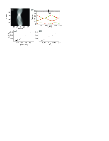
Figure 2: (a) Evolution of $|\psi_{2}|^{2}$ according to the effective one-component GP equation (13). (b) Contributions to the energies, from Eq. (II.3), $E_{k}$ (dotted curves), $E_{V}$ (dashed), $E_{\mathrm{int}}$ (dot-dashed) and total $E$ (solid) for the true two-component evolution according to Eqs. (1-2) (thick, orange curves) and effective one-component model Eq. (13) (thin, green curves). All energies are normalized by the initial total energy $E_{0}=E(t)$. The dotted lines indicate the maximum and minimum values of $E$ reached in the true two-component evolution. Their difference defines $\Delta E$. (c) The relative fluctuations of $E$ in the two-component model, normalized to the initial energy $E_{0}$, with the initial peak amplitude $f$ varied. The circled point indicates the case plotted in (a),(b). (d) The relative energy fluctuations $\Delta E/E_{0}$ with parameters the same as Fig. 1, but varying $-\delta_{c}$ and keeping $\delta_{2}=\delta_{c}$.

A quantitative comparison can be made by calculating the energy functionals:

$$E_{K} \equiv \int dz|\psi_{2}^{\prime}|^{2};$$

$$E_{V} \equiv -\delta_{c}\int dzV(z)|\psi_{2}|^{2};$$

$$E_{\mathrm{int}} \equiv \frac{1}{2}(\delta_{2}-2\delta_{c})\int dz|\psi_{2}|^{4}.$$

$$E = E_{K}+E_{V}+E_{\mathrm{int}};$$

which we plot in Fig. 2(b) for both for the effective one-component model (thin, green curves) and the full two-component prediction (thick, orange curves). One sees the curves track each other very closely and, furthermore, that all three contributions $E_{K},E_{V},E_{\mathrm{int}}$ are playing an important role in the evolution, indicating the evolution of $\psi_{2}$ is nonlinear in this case. The main deviation one observes is a very slight difference in the time scale for the oscillatory motion in the two cases. The total effective energy $E$ is necessarily conserved for the one-component model, while this quantity will only be conserved for the true two-component calculation when Eq. (13) is providing an accurate description of the evolution. Thus the fluctuations of this quantity (the solid, orange curve) is a good measure of the validity of the model and in the case there once sees these fluctuations $\Delta E$ are at a few percent level relative to the initial total energy $E_{0}$. In general, this error generally provides an estimate of the error in the oscillatory time scale.

III Applications of the model

III.1 Prediction of breathing motion

According to our model, Eq. (13), relative scattering lengths in the regime in Fig. (1) ($\delta_{c}<0$ and $\delta_{2}-2\delta_{c}>0$) will give rise to an evolution of $\psi_{2}$ analogous to a trapped interacting single component BEC. To test this model and investigate the range of its applicability, in Fig. 2(c) we plot the effective energy fluctuations for a number of cases with the same parameters as Fig. 2(a-b) but varying the initial peak relative density $f=|\psi_{2}|^{2}/\rho$. One sees that even up to $f\approx 0.7$ the energy fluctuations are still less than 10 %. In Fig. 2(d) we show a series varying the magnitudes of $\delta_{2},\delta_{c}$ (keeping $\delta_{2}=\delta_{c}<0$) and see an approximate linear dependence.

We note that because this regime generally leads to smooth breathing behavior, it may be well suited to performing controlled information processing via the two-component dynamics. In particular, the linear evolution can be predicted by decomposing the wavefunction into the harmonic oscillator states of the effective potential, and amount of nonlinearity can be controlled by the number of atoms coupled into $|2\rangle$. Furthermore, much can be borrowed from the vast existing literature on one-component BEC dynamics, including analytic predictions for the ground states in the Thomas-Fermi regime TF and the spectrum of linear excitations from this ground state oneCompExcitations .

III.2 Phase separation and vector solitons

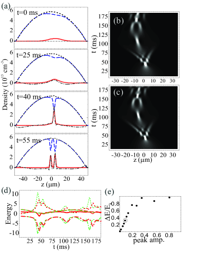
Figure 3: Numerical simulations with $\delta_{c}=-0.03,\delta_{2}=-0.09$, giving an effective attractive interaction. All conventions are the same as in Figs. 1-2 (a) Snapshots of the two component’s densities profiles and the density fluctuations. (b) Time evolution of the density profile $|\psi_{2}|^{2}$, (c) Effective one-component prediction (d) Energies. (e) Total energy fluctuations (normalized by the maximum value reached by $E_{k}$). The circled point again indicates the case shown, and the other points indicate simulations with the same parameters, but varying the initial peak amplitude of $f$.

One particularly interesting behavior of two species BECs is phase-separation phaseSepExp ; phaseSepTh which is predicted to occur when $U_{12}^{2}>U_{11}U_{22}$. In this case it is energetically favorable for the two components to separate into a series of non-overlapping domains. The manner in which this separation takes place dynamically has not been addressed in detail. According to our model Eq. (13), a species $|2\rangle$ contained in a condensate of another species $|1\rangle$ will effectively act as an attractive BEC when $\delta_{2}-2\delta_{c}<0$, which, to first order in $|\delta_{2}|,|\delta_{c}|$ is equivalent to the above phase separation criteria. Such a case ($\delta_{2}=-0.09,\delta_{2}=-0.03$) is presented in Figs. 3(a-b). One sees that, indeed, the $|2\rangle$ condensate acts as if it has attractive interactions which leads to phase separation. The wavefunction $\psi_{2}$ first collapses then suddenly splits into two distinct soliton-like structures. Fig. 3(b) shows that this evolution continues, with the the number of distinct structures alternating between 1,2 and 3. The effective one-component model here allows us to map this two-component problem onto the problem of soliton train formation in single component, attractive interaction condensates, studied both experimentally solitonTrainExp and theoretically solitonTrainTh , and thus acts as an intuitively simple and quantitatively useful guide in predicting the formation and dynamics of two-component (or vector) solitons twoCompSolitonsBEC . The effective one-component prediction is plotted in Fig. 3(c) and one sees the model gives a qualitatively accurate prediction of the behavior.

One sees in Fig. 3(d) that the quantitative error in the evolution is slightly larger than in the effective repulsive case with visible differences in the magnitude of the initial kinetic and interaction energy oscillations and especially in the magnitude and timing of later oscillations. This is primarily because the relative density $f$ grows to be quite large during the phase separation. The small $f$ prediction $\delta\rho=-\delta_{c}|\psi_{2}|^{2}$ still provides a remarkably good estimate, as shown in Fig. 3(a). While Eq. (11) would seem to imply that including a next order nonlinearity term $\sim f^{2}$ in the evolution could further improve the model, we found numerically that this did not significantly improve the quantitative accuracy. A further complication is that (the linearized versions of) the kinetic energy and quantum pressure source terms Eqs. (LABEL:eq:hydroEvol3a-8) can be more important (relative to the mean field term Eqs. (LABEL:eq:linhydroEvol3)). While explicit calculation in the case shown reveals they were still smaller than the mean field term by a factor $\sim 10$, this is enough to have some effect. Fig. 3(e) shows the energy fluctuation error (this time relative to the peak kinetic energy $E_{k}^{(\mathrm{max})}$ since the initial total energy $E_{0}$, being the sum of two large numbers of opposite sign, is near zero). One sees an approximately linear dependence of the energy fluctuations with the initial peak $f$, which saturates when the initial peak value reaches about $0.25$. For simulations with $f$ higher than the case plotted in Figs. 3(a-c), the number of solitons predicted was incorrect.

III.3 Effective repulsive potentials

In the examples we have shown so far, we have chosen $\delta_{c}<0$, since this leads to an effective trapping potential for $\psi_{2}$. The model is accurate for the opposite case as well, however it predicts (and we indeed observe) that $\psi_{2}$ is pushed to the edge of the BEC due to the effective repulsive potential. This occurs on a time scale of about 20 ms for $\delta_{c}=0.03$ and the initial BEC parameters used in this paper. The model eventually breaks down when $\psi_{2}$ reaches the BEC boundary, since the kinetic energy becomes comparable to the mean field potential $U_{11}\rho_{0}$, and the Thomas-Fermi assumption is no longer valid. Similar approaches could be constructed to account for this boundary region in certain cases (for example, in processing this was done for a case with a negligible nonlinearity term) but this is beyond our scope here.

III.4 Vanishing nonlinearity in ⁸⁷Rb

A particular case of interest in present day experiments is the hyperfine levels $|1\rangle=|F=1,M_{F}=-1\rangle$ and $|2\rangle=|F=2,M_{F}=+1\rangle$ of ⁸⁷Rb. These two levels are approximately equally trapped magnetically and have a very small inelastic collision rate inelastic , allowing them to overlap for very long times and maintain their coherence. Interestingly, the scattering lengths in this case ($\delta_{c}=-0.03,\delta_{2}=-0.06$) scatteringLengthRb are such that the effective nonlinearity vanishes and we get a very simple linear evolution of $\psi_{2}$ which could be predicted by simply decomposing the initial state into the eigenstates of the effective harmonic oscillator potential $-\delta_{c}V(z)$. There will be higher order terms $\sim|\delta_{2}|^{2},|\delta_{c}|^{2}$ which eventually introduce nonlinearity at longer times (and in fact this system is eventually phase separating multipleComponentJILA ). However the linear model could prove to be a powerful tool for predicting otherwise computationally expensive two-component evolution in two and three dimensions.

III.5 Quasi-stationary solutions

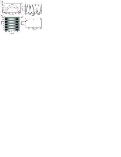
Figure 4: (a) The ground state density profile $|\psi_{2}|^{2}$ obtained by finding the effective ground state of Eq. (13) for a case with $N_{2}=0.38N$, with $|\psi_{1}|^{2}$ chosen such that the total density $\rho$ corresponds to the original ground state profile $\rho_{0}$. (b) The deviations from the initial density $|\psi_{2}(z,t)|^{2}-|\psi_{2}(z,0)|^{2}$ are quasi-periodic. (c) The deviation parameter $\Delta_{2}=\int dz(|\psi_{2}(z,t)|^{2}-|\psi(z,0)|^{2})/\int dz|\psi_{2}(z,t)|^{4}$ as versus time. (d) The maximum value reached by $\Delta_{2}$ as a function of the fraction of atoms in $|2\rangle$, $N_{2}/N$.

As a final application of our model, we consider the stationary states of the effective one-component model. In a case with only a small density $|\psi_{2}|^{2}$ the eigenstates of the harmonic oscillator potential will be stationary states of $\psi_{2}$. The ground state is simply a Gaussian wavefunction which could easily be created with a stopped light pulse processing . Our model would then predict the state written onto the wavefunction $\psi_{2}$ is then stationary and therefore quite robust with respect to storage of information. We have indeed observed numerically that the Gaussian ground state of the effective potential is stationary. Such an approach was used in vortexStorage to predict robust storage of optical vortex states in BECs in three-dimensional geometries. In this work, the stability was checked with a full calculation of the two-component evolution, but the one-component model provided a way to construct an accurate estimate for a stable configuration.

One of the motivations for stationary two-component states is the possibility of atom-atom interaction induced spin-squeezing, as proposed in spinSqueezing . In that proposal, for ²³Na, $\delta_{c}=-0.08,\delta_{2}=0$. To achieve spin-squeezing, one must have two components, each with a comparable density, overlap for a considerable time. Ideally, the mean-field dynamics should be kept to a minimum to prevent them from washing out the squeezing dynamics. This latter requirement could be accomplished by choosing the number of atoms in each component consistent with the breathe-together solutions, whereby the relative density between the two components ($f$) is constant across the BEC dynamics ; breatheTogether , while the overall density profile breathes. However, our model predicts quasi-stationary solutions for any number of atoms in $|2\rangle$. Furthermore, if one wished to write the squeezed state via slow light techniques, an inhomogenous configuration, where $\psi_{2}$ is contained in $\psi_{1}$ and vanishes at the BEC boundaries, would be essential to prevent spontaneous emission events. To our knowledge, two species BEC stationary states, with an inhomogenous relative density profile $f$, have not been previously predicted or experimentally observed.

As an example, in Fig. 4(a) we show a ground state of the effective one-component GP equation (13), obtained by propagating the equation in imaginary time, and holding the number of atoms in $|2\rangle$ $N_{2}=N\int dz|\psi_{2}|^{2}$ constant. In this case, the nonlinear term $E_{\mathrm{int}}$ is quite significant (it dominates the kinetic energy $E_{k}$ in the ground state). The density $|\psi_{1}|^{2}$ is then chosen so that the total density $\rho_{0}$ corresponds the ground state of a pure $|1\rangle$ condensate $\rho_{0}$.

A time-dependent evolution of the full two-component Eqs. (1-2) with this initial state then reveals that indeed this configuration is nearly stationary. The only observed motion is a small in-phase breathing of both components, with a magnitude governed by $\delta_{c}$. Figure 4(b) shows the variations of the density $|\psi_{2}|^{2}$ from its initial value as a function of time, which exhibits this breathing motion. Thus, not only is the motion of $\psi_{2}$ small, but the small deviations are approximately periodic and so $|\psi_{2}|^{2}$ remains near its initial value for very long times. The parameter $\Delta_{2}$, plotted in Fig. 4(c) and defined in the caption, characterizes the total deviation and is seen to be nearly periodic with a maximum amplitude of about 0.025.

We performed similar simulations for a variety of values $N_{2}$ and plotted the maximum $\Delta_{2}$ reached in each case. The results are presented in Fig. 4(d). In the limit of small $N_{2}$, where the nonlinearity is negligible the effective ground state is truly stationary. As the nonlinearity becomes more important, the ground state grows due to effective repulsive interactions, the small breathing motion occurs and we get the deviations $\Delta_{2}$. The magnitude of $\Delta_{2}$ saturates at around 0.025 (see Fig. 4(d)). The saturation occurs at the point the Thomas-Fermi solution TF of the effective one-component model becomes accurate. The saturation value should scale roughly linearly with $|\delta_{c}|$.

In the regime $N_{2}\sim N_{1}$, the effective ground state eventually becomes larger than the original condensate, in which case the present approach fails. However, in that limit, the solutions smoothly cross over into the breathe-together solutions discussed in dynamics ; breatheTogether .

IV Summary

In summary, we have derived an equation of motion for the total density fluctuations in dynamic two-component condensates. We have then used this to derive an effective one-component GP equation (13) for the smaller component, with effective potentials and interaction coefficients which depend in a simple way on the relative scattering lengths in the system. We have studied and tested the predictions of this model in both effective repulsive and attractive interactions. Our model provides an intuitively simple way to predict the dynamics of two component BECs and allow us to make correspondences to results already obtained for one-component BECs. In particular, our model provides new insight on the dynamics of phase separation and the formation of vector solitons. We noted that magnetically trapped ⁸⁷Rb provides a particularly interesting example in which the motion is governed by a simple linear Schroedinger equation, allowing simple analytic predictions of motion in cases that would otherwise require solutions of the underlying nonlinear Schroedinger equations. Finally, we have applied it to predict the existence of quasi-stationary two-component configurations. These solutions promise to be useful for applications involving information storage using stopped light as well as inducing spin squeezing in these systems. A combination of these two techniques may provide a new technique to generate squeezed light.

References

- (1) M. Inguscio, S. Stringari, and C. Wieman, eds., Bose-Einstein Condensates in Atomic Gases, Proceedings of the International School of Physics Enrico Fermi, Course CXL, (International Organisations Services B.V., Amsterdam, 1999).
- (2) H.-J. Miesner et al., Phys. Rev. Lett. 82, 2228 (1999).
- (3) T-L. Ho and V.B. Shenoy, Phys. Rev. Lett. 77, 3297 (1996); H. Pu and N.P. Bigelow, Phys. Rev. Lett. 80, 1130 and 1134 (1998); E. Timmermans, Phys. Rev. Lett. 81 5718 (1998); P. Ao and S.T. Chui, Phys. Rev. A 58, 4836 (1999).
- (4) Th. Busch and J.R. Anglin, Phys. Rev. Lett. 87, 101401 (2001).
- (5) M.R. Matthews, et al., Phys. Rev. Lett., 83 2498 (1999).
- (6) J.J. Garcia-Ripoll and V.M. Perez-Garcia, Phys. Rev. Lett. 84, 4264 (2000).
- (7) E.J. Mueller and T.-L. Ho, Phys. Rev. Lett. 88, 180403 (2002); K. Kasamatsu, et al., ibid. 91, 150406 (2003).
- (8) Z. Dutton and J. Ruostekoski, Phys. Rev. Lett. in press, cond-mat/0405159.
- (9) T. Nikuni and J.E. Williams, J. Low Temp. Phys. 133, 323 (2003).
- (10) A. Sinatra and Y. Castin, European Phys. Jour. D 8, 319 (2000).
- (11) S.D. Jenkins and T.A.B. Kennedy, Phys. Rev. A 68, 053607 (2003).
- (12) D. S. Hall, M. R. Matthews, C. E. Wieman, and E. A. Cornell, Phys. Rev. Lett. 81, 1539 (1998); ibid. 81, 1543 (1998).
- (13) B.D. Esry and C.H. Greene, Phys. Rev. A 59, 1457 (1999).
- (14) C.K. Law, H. Pu, N.P. Bigelow, and J.H. Eberly, Phys. Rev. Lett. 79, 3105 (1997).
- (15) Z. Dutton and L.V. Hau, Phys. Rev. A, in press; quant-ph/0404018.
- (16) C. Liu, Z. Dutton, C.H. Behroozi, and L.V. Hau, Nature 409, 490 (2001). D.F. Phillips, A. Fleischhauer, A. Mair, R.L. Walsworth, and M.D. Lukin, Phys. Rev. Lett. 86, 783 (2001).
- (17) S. Inouye et al., Nature 392, 151 (1998); S.L. Cornish et al., Phys. Rev. Lett. 85, 1795-1798 (2000).
- (18) S. Stringari, Phys. Rev. Lett. 77, 2360 (1996).
- (19) K.E. Strecker, G.B. Partridge, A.G. Truscott, and R.G. Hulet, Nature 427, 150 (2002); L. Khaykovich, et al., Science 296, 1290 (2002).
- (20) U. Al Khawaja, et al. Phys. Rev. Lett. 89, 200404 (2002); L. Salasnich, A. Parola and L. Reatto 91, 080405 (2003); L.D. Carr and J.Brand, Phys. Rev. Lett. 92, 040401 (2004).
- (21) A. Sorensen, L.-M. Duan, J.I. Cirac, and P. Zoller, Nature 409, 63 (2001).
- (22) D. M. Stamper-Kurn, et al., Phys. Rev. Lett. 80, 2027 (1998).
- (23) M. R. Andrews, et al., Phys. Rev. Lett. 79, 553 (1997).
- (24) G. Baym and C.J. Pethick, Phys. Rev. Lett., Phys. Rev. Lett. 76, 6 (1996).
- (25) C.J. Myatt, E.A. Burt, R.W. Ghrist, E.A. Cornell, and C.E. Weiman, Phys. Rev. Lett. 78, 586 (1997); J.P. Burke, C.H. Greene, J.L Bohn, Phys. Rev. Lett. 81, 3355 (1998). A Mathematica notebook is available at http://fermion.colorado.edu/chg/Collisions/.
- (26) J.M. Vogels, R.S. Freeland, C.C. Tsai, B.J. Verhaar, and D.J. Heinzen, Phys. Rev. A 61 043407 (2002).