Monodisperse approximation as a tool to determine stochastic effects in decay of metastable phase

Abstract

Stochastic features of decay of a metastable phase have been investigated with the help of a new monodisperce approximation. This approximation is more precise than the already used one and namely it allows to give a very simple but rather precise way to calculate dispersion of the total droplets number initiated by stochastic appearance of supercritical embryos. the derivation is done for a free molecular regime of droplets growth but the diffusion regime is also discussed.

The pioneer investigations by Wilson [1] more than hundred years ago opened systematic investigations of nucleation. But only in the last years the progress in theoretical description of nucleation allowed to put the questions of stochastic properties of the first order phase transition kinetics.

Since [5], [6], [7] considerations of stochastic properties of kinetics of the first order phase transition can be regarded as one of the actual problems to investigate.

The main statistic characteristics of the nucleation process are the mean value of the total number of droplets $N_{tot}$ and dispersion of $N_{tot}$. The mean value $\bar{N}_{tot}=<N_{tot}>$ averaged over all fluctuations and consequences of their influence on kinetics doesn’t generally differ from a value given by a theory of the averaged characteristics (TAC) [4], [10]. This property is explained in [9] and partially in [10], the derivations in [5] are illegal since they are based on an inappropriate linearization (explanation see in [10]). As for the value of dispersion of

$$\Delta=<(N_{tot}-<N_{tot}>)^{2}>$$

one can not say that it is found absolutely correctly, the deviation between numerical simulations and results of [5] is about 10 percent, the error in [10] is practically absent, but when the procedure from [10] is applied to other regimes of droplets growth (not for the free molecular one) the error can increase up to 10 percent. So, the task to propose a way to calculate dispersion remains rather actual.

One has to choose the style of determination of dispersion of the nucleation process. The traditional way is to start with the iteration solution and to determine the dispersion on the base of iteration. But this way can not lead to a suitable result. Really, the deviation of the square of dispersion $D$ from the standard value

$$D_{standard}=2N_{tot}$$

can be attained only by reaction of the formation of new droplets at the latest moments of nucleation period on the excess of the droplets formed in the first moments of nucleation period. But the reaction of the formation of new droplets on formation of other already existing droplets appears only in the second iteration in frames of standard iteration procedure (see [2]). The second iteration can not be analytically calculated even in the theory with averaged characteristics, only the number of droplets in can be determined analytically.

So, one has to come to some method of calculation of dispersion which is based on some model behavior of supersaturation. An approach of such type was used in [5], [6]. In the cited papers the approximation proposed in [3] was used to calculate the stochastic effects. This approximation is the following: during the first half of nucleation period the droplets are formed under the ideal supersaturation, later all remaining droplets are formed under the vapor consumption by the droplets from the first half. This approximation originally was used in [3] only for some rough estimates necessary for justification of strong inequalities necessary to construct the mathematical models of kinetics.

The mentioned model belong to the class of models with a fixed boundary. Namely the boundary between the first half and the second half has a fixed value - the transition between cycles occurs in the fixed moment of time.

One can see that the two cycle models with a fixed boundary aren’t too suitable for calculation of stochastic properties of the phase transition kinetics. Really, the stochastic deviations of characteristics of the first cycle means that in the prescribed approximation the parameters coming from the evolution before the boundary will differ from the value in the theory based on the averaged values.

But the model used in investigation of stochastic effects was chosen namely for the theory with averaged characteristics. Why shall it work with other values of parameters? Certainly, there is no reason for applicability of the model in such situation. This is the main contradiction in the application of two cycle model with a fixed boundary in investigation of stochastic properties.

Fortunately the situation of decay in a free molecular regime of droplets growth can be roughly described on the base of the model with a fixed boundary. This possibility is explained by existence of specific zone - the buffer zone [10]. The description of stochastic effects on base of the mentioned approximation requires some rather complex constructions because the buffer cycle complicates construction. The precision of calculations isn’t too high because the buffer zone isn’t too long and can be extracted with a certain imagination.

Alternative possibility is to use the model with a floating boundary. In these models the boundary is determined from equations corresponding to the attaining of some values of some characteristics of process. The model of monodisperce spectrum [8] belongs to this class.

The property of internal time in the kinetics of decay observed in [10], [11] states that the system can wait so long as possible for appearance of essential quantity of droplets in the system and nothing will be changed in nucleation kinetics. The process will simply be shifted in the time scale.

In the model of monodisperse spectrum with a floating boundary the number of droplets appears as the determining characteristic. In our therminology the determining parameter is the characteristic which fixed value has to be attained at the boundary.

What type of model with the floating boundary we have to choose? Certainly, one can propose the simple generalization of the model used in [10]: until the boundary the rate of appearance of droplets is ideal one and later the evolution is governed by droplets appeared before the boundary. If we suppose that the rate of droplets formation is ideal (unperturbed by the vapor consumption) until some moment, then we have to take into account that the average amplitude of spectrum for the droplets formed in the first cycle is one and the same for all of them. Then the subintegral function in expression for $g$ has a special power behavior. Namely this behavior is the base to determine the boundary (not only the number of droplets in the first cycle determines the boundary). At least one has to take into account all four first momenta of the spectrum. So, on one hand the theory becomes very complex. On the other hand the constant value of spectrum in the first cycle is violated by stochastic fluctuations and the approximation can be violated also. This is a certain disadvantage of th emodel. So, this model can not be effectively used.

Also here appears a question: what characteristic will determine the boundary? Or one can put a question: what equation on the boundary should be written? There is no clear answer on these questions.

So, the simplest model satisfying our requirements is the monodisperse model. Here we don’t face such difficulties as in the models described previously because namely the number of droplets stands both in monodisperse approximation and in Gaussian distribution for the number of droplets formed during the first cycle. Also the number of droplets is the determining characteristic here.

Recall briefly the monodisperse approach. The evolution equation after rescaling can be written as [8]

$$g(z)=\int_{0}^{z}(z-x)^{3}\exp(-g(x))dx$$ (1)

where unknown function $g$ is the renormalized value of the number of molecules in a new phase.

In monodisperce approximation one can use for $g$ the model where all ”essential” droplets have one and the same size, i.e.

$$g(z)\sim z^{3}$$

The number of essential droplets $N_{ess}$ is parameter of the model.

The total number of droplets $N_{tot}$ is calculated as

$$N_{tot}\sim\int_{0}^{\infty}\exp(-g(x))dx$$

Precise solution of (1) gives

$$N_{tot}=1.28$$

In the standard monodisperse approximation

$$g(z)=N_{ess}z^{3}$$

$$N_{ess}=1/4$$

and

$$N_{tot}=\int_{0}^{\infty}\exp(-x^{3}/4)dx\approx 1.25$$

We shall start with numerical results for the number of droplets formed in the process of decay. The results for the total number of droplets are drawn in Figure 1.

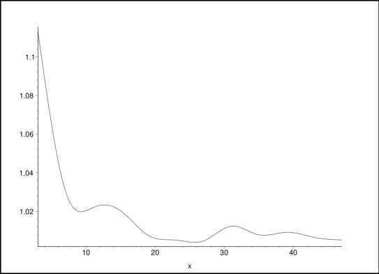
Figure 1: Numerical solution. The number of droplets in the units of the number predicted by the mean values theory as a function of the volume of the system (or the number of droplets in MVT).

One can note here that practically immediately after the initial moment of time the number of droplets is the mean value predicted by the mean values theory (MVT). This isn’t valid only for the first few droplets.

Now we shall present results in the mean values of droplets for the model with monodisperse spectrum. Here the vapor consumption occurs by the monodisperse peak $N(\Delta x/4)$ as it prescribed by the monodisperse variant of MVT [8].

One can prove that in all monodisperse models the mean number of droplets coincides with the corresponding values calculated in MVT.

At this step there appears a little discrepancy because the monodisperse spectrum in the monodisperse variant of MVT begins to act at the very beginning and we have to wait until the moment when $N_{tot}/4=1/4$ will appear. So, a little shift in the mean value of droplets predicted by MVT appears. Since we draw relative numbers, i.e. $<N>/N_{tot}(V=\infty)$ there will be no error.

The results are drawn in Figure 2.

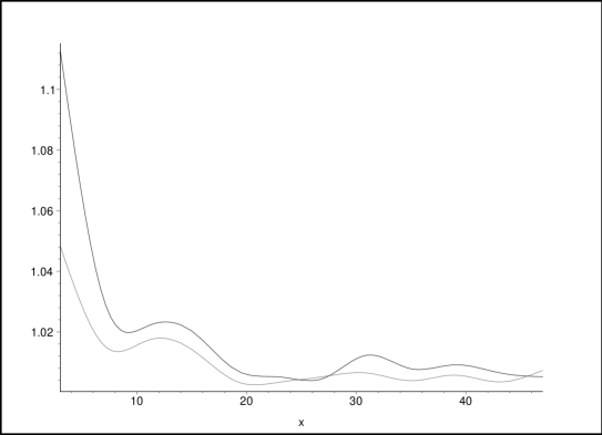
Figure 2: Numerical solution and momodisperse approximation. The number of droplets in the units of the number predicted by the mean values theory.

Here there are two curves. The curve with greater flash at small $x=V$ corresponds to the precise solution, the second curve comes from the monodisperse model.

We see that the monodisperse model gives practically the same behavior of the mean value of the droplets number except the small $V$.

Numerical errors can be evidently seen when we compare our results with a model where the first droplet appears stochastically and all other droplets later appear according MVT. The results are shown in Figure 3 where the lower curve comes from this model and two upper curves have been already drawn in the Figure 2.

Figure 3: Numerical solution. The number of droplets in the units of the number predicted by the mean values theory.

Certainly, the last model can not give anything more that MVT (because the system will simply wait until the appearance of the first droplet and we can put $t=0$ at this very moment). Certainly there appears a little peak corresponding to the first droplet (That’s why the dependence over volume $V$ of the system still exists.) We see that here it is impossible to analyze the tails of dependencies (at big volumes), they lies in the frames of error of numerical accuracy.

The effects of discrete number of droplets can be seen from the following simple model: The first droplet appears stochastically and later all other droplets appear regularly when the integral of the nucleation rate over time attains integer numbers. Then results are shown in figure 4.

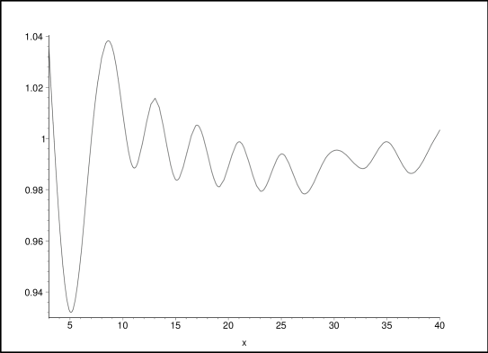
Figure 4: Solution of the discrete regular model. The number of droplets in the units of the number predicted by the mean values theory.

We see that the deviations due to the discrete character of the droplets number are even more essential than other effects. But in reality they do not take place because all $N_{eff}$ droplets appeared independently and stochastically and these shifts will compensate each another.

Now we shall turn to the investigation of dispersion.

The results of dispersions for precise solution and for monodisperse approximation (for every model there are two dispersions: one in units of $<N_{tot}>$ and another is in the units of $<N_{tot}(V=\infty)>$, but for such big values of $<N_{tot}>$ they practically coincide) are shown in figure 5.

Figure 5: Dispersions for precise solution (the upper curves) and for the monodisperse approximation (the lower curve).

The dispersion in the monodisperse model can be easily calculated. Really, the first part of droplets, i.e.

$$N_{eff}=1/4$$

has no dispersion

$$D_{eff}=0$$

because the system simply waits until there appears the $N_{eff}$ droplets precisely. This behavior is prescribed by the absence of the ”external” time in the situation of decay. The system has only the ”internal time”. It waits until there will be enough droplets to ensure the beginning of the vapor consumption. This approximate picture is more realistic than a picture with fixed moment of the boundary between the cycle of appearance of the main consumers and the cycle of the real intensive consumption of vapor.

The droplets appeared during the cycle of consumption are born under the known supersaturation and, thus, under the known rate of nucleation. So, we have the free appearance of droplets with known number of possible acts of appearance or the appearance with a known time lag of the cut-off. So, the dispersion will be equal to the dispersion of appearance of the free droplets with a mean value

$$<N_{rest}>=<N_{tot}-N_{eff}>=1.28-0.25=1.03$$

So, the $D$ is

$$D_{rest}=2<N_{rest}>$$

The total dispersion (after the combination of gaussians) will be found from

$$D_{total}=D_{eff}+D_{rest}=1.03$$

Being referred to the standard $D$ which is two total numbers of droplets $D_{standard}=2N_{tot}=2*1.28$ it gives the relative dispersion according to the following expression

$$D_{rel}=1.03/1.28=0.75$$

We see that the result for dispersion of the monodisperse approximation isn’t too close to the real solution. What is the matter of this discrepancy? Really, we see that the monodisperse approximation which has been used (let us call it the ”standard monodisperse approximation”) has some disadvantages:

• Already all essential droplets appear at the initial moment of time. It leads to the inequality of the real mean value of ”essential” droplets and the coordinate of monodisperse peak.

• We have to keep the balance of substance but since the mean coordinate (size) of effective droplets is less than the coordinate of monodisperse peak then the number of essential droplets in monodisperse approximation have to be less than the real number of essential droplets. This shows why the real dispersion is less than the result given by the standard monodisperse model.

So, we have to put the coordinate of monodisperse peak to the real mean coordinate of ”essential” droplets. Then we come to the following model

• At $z=l$ the monodisperse peak is formed. It contains $N_{eff}=1*l+1*l$ droplets (here it is taken into account that the amplitude here is unperturbed and it equals to $1$ and the peak has rather symmetric form).

• The total number of droplets is calculated as

  $$N_{tot}\approx N_{tot\ 1}=l+\int_{0}^{\infty}\exp(-2lx^{3})dx$$

  or

  $$N_{tot}\approx N_{tot\ 2}=2l+\int_{l}^{\infty}\exp(-2lx^{3})dx$$

This model will be called as the ”primitive monodisperse model”.

Unfortunately this model can not give the correct value of the total number of droplets. The value $N_{tot}$ as a function of $l$ is drawn in figure 6.

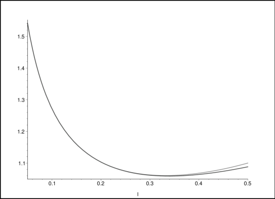
Figure 6: The total number of droplets as a function of parameter $l$ in a primitive monodisperse model.

Here two curves for $N_{tot\ 1}$ and for $N_{tot\ 2}$ are drawn. We take the relative values referred to the precise value $N_{tot}=1.28$. They are so close that one can not separate them. Only at the tail one can see the thick line corresponding to the little deviation $N_{tot\ 1}$ from $N_{tot\ 2}$.

We see that the result is greater than $1.1$ even in the minimum corresponding to $l=0.33$. Namely this value is the most suitable value of parameter $l$ in the primitive monodisperse model.

The value of minimum of the droplets number is important not only because it is the closest number to the real value $1.28$ but also because it is the minimum and the minimum in the droplets number corresponds to the minimum of the free energy of the total system. So, this property can be effectively used and we shall seek in future the values of such minima in more sophisticated models.

The evident weak feature of this model is that the position of the monodisperse peak is put directly in the middle of the period of formation of all effective droplets. It supposes the relative symmetry of the vapor consumption of all effective droplets. Certainly it isn’t true, one can see on the base of the first iteration that the subintegral function resembles $(z-x)^{3}$ and isn’t symmetric. So, now we shall introduce the arbitrary shift of the position of the peak and formulate the next model as following:

• The lenght of monodisperse peak is $z=2*l$. It contains $N_{eff}=1*l+1*l$ droplets (here it is taken into account that the amplitude here is unperturbed and it equals to $1$).

• The position of the peak is formed at $z=2*l-b$ with the parameter $b$. Earlier it was $b=l$.

• The total number of droplets is calculated as

  $$N_{tot}\approx N_{tot\ 1}=2l-b+\int_{0}^{\infty}\exp(-2lx^{3})dx$$

  or

  $$N_{tot}\approx N_{tot\ 2}=2l+\int_{b}^{\infty}\exp(-2lx^{3})dx$$

• The value of $b$ is determined to touch the value $1.28$ at the minima over $l$

This model will be called as the ”advanced monodisperse model”.

The calculations give $b=0.33$ and the function $N_{tot}$ over $l$ at $b=0.33$ is drawn in figure 7

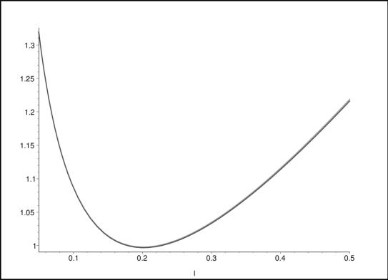
Figure 7: The total number of droplets as a function of parameter $l$ in the shifted monodisperse model at $b=b_{0}\equiv 0.336$.

Here also two curves with the same meaning coincide.

The number of effective droplets here is $N_{eff}=0.4$.

Theoretical result originally going from the floating monodisperse approximation (see [8]) is

$$b=2l-(1/4)*2l=0.3$$

Here $1/4$ is the same as $N_{ess}$ in our first model.

Now we shall clarify the physical sense of this approximation. One can see that

$$\int_{0}^{b}\rho^{3}d\rho\approx\int_{b}^{0.4}\rho^{3}d\rho$$

We can require that the quantity of substance in the ”left” part of monodisperse spectrum (i.e. in the droplets appeared before the peak) equals to the quantity of substance in the ”right” part of spectrum (i.e. in the droplets appeared after the peak of spectrum). Then we come to the practically same results as before.

It is very easy to get the results for dispersion in this model.

$$<N_{rest}>=<N_{tot}-N_{eff}>=1.28-2*l=0.88$$

So, the dispersion is found from

$$D_{rest}=2<N_{rest}>$$

The total dispersion (after the combination of gaussians) is given by the following expression

$$D_{total}=D_{eff}+D_{rest}=0.88$$

Being referred to the standard dispersion which is two total numbers of droplets it gives the relative dispersion according to

$$\gamma=0.88/1.28=0.68$$

This value is rather close to the result of computer experiments. Then we can fulfill some formal summations analogous to [10] due to the self similarity of the process of nucleation (see [11]) and get the result which practically coincides with numerical simulation.

Now we shall turn to numerical simulation for the last model.

The mean number of droplets is drawn in Figure 8.

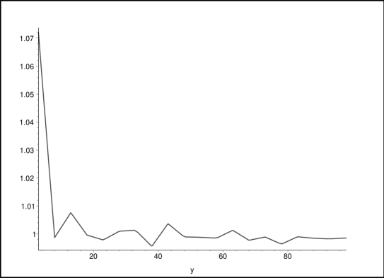
Figure 8: The mean number of droplets as a function of the volume of the system.

The dispersions are drawn in Figure 9.

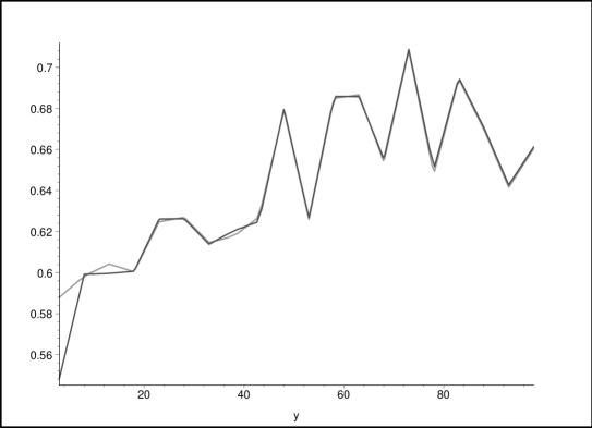
Figure 9: Relative dispersions as functions of the volume of the system.

We see that numerical results of this model are practically the same as the results of computer simulation of the process in initial formulation.

The use of monodisperse approximation in investigation of stochastic effects of nucleation has certain advantages. The first is the real simplicity of this method. Really, two summations and multiplications lead to a final result. But this simplicity isn’t only a reduction of amount of calculations. Behind this simplicity lies the real physics of manifestation of stochastic effects in decay of metastable state.

The process of decay can be qualitatively described as following. The system waits for formation of necessary amount of droplets which later will be the main consumers of vapor in the whole nucleation period. Later all these droplets will be the main consumers of all surplus metastable phase. Every droplet consumes approximately equal amount of metastable phase.

The process of phase transition has a three cycle structure. In the general period of the whole phase transition the period of formation of the main consumers of vapor, i.e. the nucleation period, can be extracted. In the nucleation period the sub-period of formation of the main consumers of vapor at nucleation period, i.e. the initial period of nucleation, can be extracted. The further extraction doesn’t take place. As it has been shown the system simply waits until formation of the necessary number of droplets characteristic for the initial cycle. The initial cycle can not be further divided, at least in frames of description of stochastic effects by means of dispersion and the mean value of the droplets number.

Certainly, this picture is approximate and in some rare cases it can be violated. In principle it is possible that the total number of droplets is less even than $N_{ess}$. But since $N_{ess}$ is seriously less than $N_{tot}$ the probability of such event is extremely low. Account of dispersion of initial period is analogous to [9] where it was done for the smooth behaviour of external conditions. Also one can found it in [10] but since there the model with a fixed boundary is studied, some evident modifications have to be performed.

When we are interested in more specific characteristics such as higher momenta of the differential distribution function then one has to fulfill quite the same extraction of sub-sub-periods in initial sub-period. Practically nothing will be changed. So, one can observe the chain of sub-periods responsible for deviations in values of high momenta of distribution. This chain is limited by the formation of the first droplet.

In some regimes of the droplets growth one can observe the direct influence of the moment of formation of the first droplet on the nucleation kinetics. This picture will be published separately.

Now we shall turn to investigation of the diffusion regime of droplets growth. This consideration is rather formal one because kinetics of nucleation in such a regime is based on some other features (see [12]). But we still perform calculations to see specific features of stochastic effects in this case.

To investigate the process of decay in diffusion regime of droplets growth one can also use the modified monodisperse approximation.

To get the monodisperse approximation we consider equation

$$g(z)=\int_{0}^{z}(z-x)^{3/2}\exp(-g(x))dx$$

The remormalization with the absence of coefficient corresponds to more natural expression for the number of droplets in monodisperse peak.

The number of droplets in first iteration is given by

$$N_{1}=\int_{0}^{\infty}\exp(-\frac{2}{5}x^{5/2})dx=1.27$$

Traditional monodisperse approximation requires to put the monodisperse spectrum at $z=0$. The number of droplets $N_{mono}$ in the monodisperse peak is chosen to satisfy the first iteration and looks like

$$N_{mono}=(2/5)z$$

It corresponds to the value of the boundary $p=0.4*1.25$ between the cycle of formation of the main consumers during the period of nucleation and the rest droplets. Here $1.25$ is the charateristic lenght of spectrum in this renormalization.

In this approximation the dispersion will be calculated according to

$$D=2(1.27-0.4)/1.27*N$$

where $N$ is the mean value of droplets. So, the relative dispersion will be

$$\gamma=(1.27-0.4)/1.27=0.685$$

This value is too far from the real value but still this value is closer to the real value $0.45$ of dispersion than the result given by the direct application of recipe given in [5] to the diffusion regime.

Now we shall use more realistic monodisperse approximation. Why the coordinate of monodisperse spectrum is put to $z=0$? Certainly, there is no strong motivation of such choice except notation that $z=0$ corresponds to the maximum value of spectrum and the maximum value of subintegral function in expression for $g$.

As one of contre-arguments one can say that $z=0$ leads to the absolutely unsymmetric monodisperse spectrum. So, it isn’t too reasonable to choose $z=0$.

Instead of this choice we shall leave the coordinate of spectrum as a free parameter. Namely we suppose that in the monodisperse spectrum there is $2*l$ droplets. since $l$ is small in comparison with $1.25$ one can state that these droplets were formed at ideal supersaturation. Then the upper boundary of the region of formation of monodisperse peak is $2l$. We suppose that the monodisperse spectrum is formed at $2l-b$. Here $b$ is a free parameter.

The total number of droplets is calculated as

$$N_{tot}=2l+\int_{b}^{\infty}\exp(-2lz^{3/2})dz$$

In addition we have to suggest a recipe to determine parameter $b$. One can prove that at arbitrary $0<b<2l$ the value $N_{tot}$ as a function of $l$ has minimum. It is clear that this minimum is the most profitable from the energetical point of view. So, the real evolution corresponds to the choice of $l,b$ giving minimum of $N_{tot}$.

We shall require that the value of munimum has to be equal to the real number of droplets. One can use as this number the number of droplets in the first iteration.

Calculations give $l=0.35$, $b=0.65$. So, dispersion will be

$$\gamma=(1.27-2*0.35)/1.27=0.448$$

This value coincides with the result of numerical simulation.

One can note that the value $N_{tot}$ as $1.27$ which is given by the first iteration corresponds to the similarity of spectrum. Namely this similarity was already used to refine the results of the two cycle model.

We see that the value $2l$ of the ”length” of essential part of spectrum is more than $60$ percents of the lenght of th etotal spectrum. It means that the majority of droplets participates in vapor consumption during the nucleation period. This corresponds to another structure of nucleation kinetics presented in [12].

References

- [1] Wilson C.T.R. Condensation of water vapour in the presence of dust air and other gases. - Phil. Trans., 1898, v.189A, N11,p.265 Wilson C.T.R. On the condensation nuclei produced in gases by the action of Roentgen rays, uranium rays, ultraviolet rays and other agents. - Phil. trans., 1899, v.192A, N9, p.403 Wilson C.T.R. On the comparison efficiency as condensation nuclei of positively and negatively charged ions - Phil.Trans., 1900, v.193A, p.289
- [2] Kuni F.M., Grinin A.P., Kurasov V.B., Heterogeneous nucleation in vapor flow, In: Mechanics of unhomogenenous systems, Ed. by G.Gadiyak, Novosibirsk, 1985, p. 86 (in Russian)
- [3] V.B. Kurasov Universality in kinetics of the first order phase transitions, SPb, 1997, 400 p. (in English)
- [4] Kurasov V. Phys. Rev. E, vol. 49, p. 3948 (1994)
- [5] Grinin A.P., F.M.Kuni, A.V. Karachencev, A.M.Sveshnikov Kolloidn. journ. (Russia) vol.62 N 1 (2000), p. 39-46 (in russian)
- [6] Grinin A.P., A.V. Karachencev, Ae. A. Iafiasov Vestnik Sankt-Peterburgskogo universiteta (Scientific journal of St.Petersburg university) Series 4, 1998, issue 4 (N 25) p.13-18 (in russian)
- [7] Grinin A.P., Kuni F.M., Sveshnikov A.M. Koll. Journ., 2001, volume 63, N6, p.747-754
- [8] Kurasov V.B., Deponed in VINITI Manuscript 2594B95 from 19.09.95, 28p.
- [9] Kurasov V.B. to be published
- [10] Kurasov V.B. Preprint cond-mat@xxx.lanl.gov get 0410616
- [11] Kurasov V.B. Preprint cond-mat@xxx.lanl.gov get 0410043
- [12] Kurasov V.B., Physica A 226 (1996) 117