Heisenberg spins on a cone: an interplay between geometry and magnetism

Abstract

This work is devoted to the study of how spin texture excitations are affected by the presence of a static nonmagnetic impurity whenever they lie on a conical support. We realize a number of novelties as compared to the flat plane case. Indeed, by virtue of the conical shape, the interaction potential between a soliton and an impurity appears to become stronger as long as the cone is tighten. As a consequence, a new kind of solitonic excitation shows up exhibiting lower energy than in the absence of such impurity. In addition, we conclude that such an energy is also dependent upon conical aperture, getting lower values as the latter is decreased. We also discuss how an external magnetic field (Zeeman coupling) affects static solitonic textures, providing instability to their structure.

1 Introduction and Motivation

Two-dimensional (2D) Heisenberg-like spins models has attracted a great deal of efforts in the last decades. Actually, they have been applied to study a number of magnetic materials displaying several properties[1]. For instance, the continuum version of the isotropic 2D Heisenberg lattice (so-called nonlinear $\sigma$ model- NL$\sigma$M) is useful for investigating properties of quasi-planar isotropic magnetic samples in the long-wavelenth and zero-temperature limits. In this case, the nonlinearity of the continuum theory supports static excitations with associated finite energy, the so-called Belavin-Polyakov solitons[2]. Such pseudo-particles, like the kinks of sine-Gordon or the ’t Hooft-Polyakov monopoles of Georgi-Glashow model have their stability guaranted by topological features of the model rather than the equations of motion (for a review, see, for example Ref.[3]). In fact, the presence of topologically stable nonlinear excitations in magnetic systems may render the latter ones interesting new phenomena. As a example, we quote the role played by vortex pair dissociation which induces a topological phase transition in the sample, at the temperature $T_{\rm BKT}$, even though no long range order is established[4].

On the other hand, even the purest samples contain impurities (and defects, imperfections, etc) whose presence may give rise to important new properties. This is the case, for instance, of artificially dopped semiconductor materials. In magnetic materials, impurities may be considered for improving (magnetic impurity) or for vanishing (nonmagnetic, spinless) local magnetic interaction at the positions where they were placed. However, recent reported results have found that the antiferromagnetic correlations around a spin vacancy are not destroyed, rather they appear to be increased [5, 6, 7]. Such a result has leads to the appearance of a new type of soliton whose energy is lower than its counterpart in the absence of the spinless impurity[6, 7, 8]. This ‘more fundamental soliton’ has been theoretically [7, 8, 9, 10, 11] studied and observed in experiments[6].

In the work of Ref.[8], the NL$\sigma$M supplemented by a static nonmagnetic impurity potential was applied to study such a new soliton. In spite of the investigation be carried out in the low frequency limit, its results were shown to be in excellent agreement with numerical and discrete lattice ones [6, 7]. Actually, as presented in Ref.[8], an attractive potential takes place between the soliton and the spin vacancy as long as they are sufficiently close. In addition, such a potential is expected to give rise to oscillating solitons with definite frequencies around the static impurity [10] and could be taken as a trapping mechanism for solitonic excitations[12].

The discussion presented above is mainly concerned to magnetic systems defined on a flat plane, i.e., curvatureless manifold. Nevertheless, recent works have dealt with Heisenberg-like spins on curved background, e.g., cylinders, cones, spheres, thorus. In these cases, a number of new phenomena have been described, like the geometrical frustration on spin textures induced by curvature and/or by non-trivial topological aspects of the space manifold, say, angular deficit in cones, area deficit in planes with a disk cut out, and so forth (see, for example, Refs.[15, 13, 14, 16]). Actually, the study of such systems may be of considerable importance for practical applications, for example, in connection to soft condensed matter materials[15] (deformable vesicles, membranes, etc), and also to artificially nanostructured curved objects (nanocones, nanocylinders, etc) in high storage data devices[17, 18].

Here, we shall consider the Heisenberg spin system lying on a conical background in the presence of a static spinless impurity. As we shall see, by virtue of an interplay between geometry (cone aperture angle, $\alpha$) and magnetism, soliton-like excitations experience a collective effect of impurity and geometry so that, the potential between both objects appears to become stronger as the cone is tighten. As a consequence, we also realize that new solitonic excitations appear exhibiting lower energy as $\alpha$ is decreased. We discuss on possible consequences of these results whenever compared to the flat plane case. Furthermore, we analyse the effect of an external magnetic field on static solitons and show that such a coupling becomes these excitations unstable.

2 The model and the influence of spin vacancy on solitonic excitations on the cone

We shall start by considering the continuum limit of the 2D isotropic Heisenberg spins model supplemented by the presence of a static spin vacancy potential like below:

$$H=\frac{J}{2}\,\int\,d\rho^{2}\left[(\partial_{t}\vec{n})^{2}-(\nabla\vec{n})^{2}\right]\,V(\vec{\rho})\,,$$ (1)

with $J>0$ representing the antiferromagnetic coupling (in the static limit, $\partial_{t}\vec{n}=0$, and with $J<0$, the model above could describe a ferromagnetic system), while the integral is evaluated over a conical surface with coordinates $\vec{\rho}=(\rho,\tau)$ related to the usual cylindrical ones, $(r,\phi)$, by:

$$\rho=\frac{r^{\beta}}{\beta}\,,\qquad\tau=\beta\varphi\,.$$

In addition, $\vec{n}=[(\sin\theta\cos\Phi;\sin\theta\sin\Phi;\cos\theta)]$ is the Néel spin vector state, with independent variables $\theta(\vec{\rho},t)$ and $\Phi(\vec{\rho},t)$. Furthermore, following the work of Ref.[8], we may write the non-magnetic impurity, $V(\vec{\rho})=V_{I}(\vec{\rho})$, as:

$$V_{I}(\vec{\rho})=\left\{\begin{array}[]{l}0\quad{\rm if}|\vec{\rho}-\vec{\rho}_{I}|<A\\ 1\quad{\rm if}|\vec{\rho}-\vec{\rho}_{I}|\geq A\end{array}\right.\,,$$ (4)

with $A=a^{\beta}/\beta$, $a$ is the lattice spacing parameter.

Then the dynamical equations which follows from Hamiltonian (1) read like (hereafter, $m=\cos(\theta)$):

$$\frac{\partial\,m}{\partial\,t}=V_{I}(\vec{\rho})\left[\nabla^{2}\Phi-\frac{2m}{(1-m^{2})}(\nabla m)\cdot(\nabla\Phi)\right]-\nabla\Phi\cdot\nabla V_{I}(\vec{\rho})\,,$$ (5)

$$\frac{\partial\,\Phi}{\partial\,t}=V_{I}(\vec{\rho})\left[\nabla^{2}m+\frac{m}{(1-m^{2})}(\nabla m)^{2}+m(1-m^{2})(\nabla\Phi)^{2}\right]-\nabla m\cdot\nabla V_{I}(\vec{\rho})\,.$$ (6)

A straighforward calculation also gives:

$$\nabla V_{I}(\vec{\rho})=(\beta\rho)^{1-1/\beta}\,\frac{a^{\beta}}{\beta}\left[\hat{e}_{\rho}\cos(\gamma-|\tau-\tau_{I}|)+\hat{e}_{\tau}\sin(\gamma-|\tau-\tau_{I}|)\right]\delta(\vec{\rho}-\vec{\rho}_{I}-\vec{A})\,.$$ (7)

As may be easily checked, whenever we take the static limit in eqs. above in the absence of the spin vacancy (thus, $V(\vec{\rho})=1$ everywhere in Hamiltonian (1), etc), such eqs. are solved by static spin textures lying on the cone with the profiles (see Ref.[16]):

$$m(\vec{\rho})=m_{0}(\rho)=\frac{\rho^{2}-\rho_{0}^{2}}{\rho^{2}+\rho_{0}^{2}}\,,\qquad\Phi(\vec{\rho})=\Phi_{0}(\tau)=\tau\,,$$ (8)

which represent solitonic excitations with radius $R=(\beta\rho_{0})^{1/\beta}$ and associated energy $E_{0}=4\pi\,J\beta$. Thus, in the $\beta\to 1$ limit (usual planar case), the results above recover those describing the so-called Belavin-Polyakov solitons, presenting radius $R$ and energy $E_{BP}=4\pi\,J$ (see Ref.[2]). Then, solutions (8) are the conical counterparts of the Belavin-Polyakov solitons.

As a first result, notice that such objects present lower energy whenever lying on a cone. Thus, if we consider a planar surface with one or more imperfections in conical shape (cusps, etc) then it is expected that solitonic excitations will tend to nucleate around the apices of such cusps, once for presenting such a configuration a smaller amount of energy is demanded. This could be viewed as a geometrical pinning of solitons.

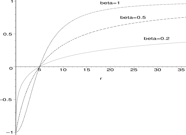
Figure 1: Shows solitonic profile $m=m_{0}$ as function of distance, $r$, centered at the apex cone ($\vec{r}=\vec{0}=\vec{\rho}$). Note how such a behavior changes as $\beta$ decreases. Here, we have taken $R=5a$.

In addition, we should notice that the magnetization variable, $m$, behaves in a peculiar way on the cone whenever compared to the flat plane case. Figure 1 shows how $m=m_{0}$ varies with distance, $r$. Notice that as $\beta$ decreases (cone is tighten) spins located from the apex to $r=R$ (or, equivalently $\rho=\rho_{0}$), present stronger variations than those outside soliton radius, $r>R$. Physically, such an asymmetry in the variations comes about by the area deficit (brought about by the angular deficit): as $\beta$ gets smaller the area on the cone, say, from the apex to $\rho_{0}$, also decreases, lefting minor space to spins turn from $m_{0}=-1$ to $m_{0}=0$. In the limit of very small $\beta$, magnetization should abruptly pass from $m_{0}=-1$ to $m_{0}=0$, while the change from $m_{0}=0$ to $m_{0}=1$ would be performed in a so smoothly way.

As a first step forward, let us see how spin vacancy affects static solitons. For that, let us consider that the interaction of spins with such a static impurity is much less than spin-spin coupling. Then, we shall take: $m(\vec{\rho})=m_{0}(\rho)+m_{1}(\vec{\rho})$ and $\Phi(\vec{\rho})=\Phi_{0}(\tau)+\Phi_{1}(\vec{\rho})$ where $(m_{0},\Phi_{0})$ are given in (8), while $(m_{1},\Phi_{1})$ are small corrections to the former ones, provided by $V_{I}$. In this case, we may linearize eqs. (6) with respect to $m_{1}$ and $\Phi_{1}$ for $\rho\geq\,a^{\beta}/\beta$, obtaining:

$$\nabla^{2}\Phi_{1}-2\frac{m_{0}\vec{\nabla}\,m_{0}}{(1-m_{0}^{2})}\cdot\vec{\nabla}\Phi_{1}=-\frac{a^{\beta}}{\rho_{I}}\,\sin(\gamma)\delta(\vec{\rho}-\vec{\rho_{I}})\,,$$ (9)

$$\nabla^{2}\,m_{1}+2\left[\frac{(\nabla\,m_{0})^{2}+m_{0}\vec{\nabla}m_{0}\cdot\vec{\nabla}}{(1-m_{0}^{2})}\right]m1+2m_{0}(1-m_{0}^{2})\vec{\nabla}\Phi_{0}\cdot\vec{\nabla}\Phi_{1}=$$

$$\hskip 199.16928pt-\frac{4\rho_{0}^{2}\rho_{I}\,a^{\beta}}{(\rho_{I}^{2}+\rho_{0}^{2})^{2}}\,\cos(\gamma)\,\delta(\rho-\rho_{I})\,.$$ (10)

Now, considering that the spin vacancy is located at the soliton center, say, $\vec{\rho_{I}}=(0,0)$ (conical apex), then $\sin(\gamma)=0$, yielding $\Phi_{1}={\rm constant}$ for eq. (9), while (10) becomes:

$$\nabla^{2}m_{1}+2\frac{(\nabla\,m_{0})^{2}+m_{0}\vec{\nabla}\,m_{0}}{(1-m_{0}^{2})}\cdot\vec{\nabla}\,m_{1}=0\,,$$

or still, by recalling that the 1st derivative term disappears if we change to $m_{0}\equiv{u}$, we get:

$$\frac{d^{2}\,m_{1}}{du^{2}}+\frac{2\,m_{1}}{(1-u^{2})}=0\,,$$ (11)

whose solutions are the trivial one, $m_{1}=0$ and:

$$m_{1}(m_{0})=c_{1}(1-m_{0}^{2})+c_{2}\left[m_{0}+\frac{1}{2}(1-m_{0}^{2})\,ln\left(\frac{1+m_{0}}{1-m_{0}}\right)\right]\,,$$

with $c_{1}$ and $c_{2}$ being constants to be determined by the solitonic characteristics. Indeed, by demanding that as $\rho\to\infty$, $m=m_{0}+m_{1}\to 1$ we must impose $c_{2}=0$. Then, the complete solutions in the presence of the spin vacancy are the following:

$$m_{P}=m_{0}\,,\quad\Phi_{P}=\Phi_{0}\,,$$ (12)

$$m_{I}=m_{0}+c_{1}(1-m_{0}^{2})\,,\quad\Phi_{I}=\Phi_{0}\,.$$ (13)

Actually, we should notice that the presence of the nonmagnetic impurity support both of the two solitonic excitations above, similarly to what happens even in the usual plane case, Ref.[8]. Their energy read as below:

$$E_{j}=\frac{J}{2}\int_{0}^{2\pi\beta}\,d\tau\int_{a^{\beta}/\beta}^{\infty}\left[\frac{[\vec{\nabla}(m_{0}+m_{j})]^{2}}{(1-m_{0}^{2})}+(1-m_{0}^{2})(\vec{\nabla}\Phi_{0})^{2}\right]\rho\,d\rho\,,$$ (14)

where $j$ stands for soliton type, say, $j=I,P$, while the lower cut-off in the $\rho$-integral, $a^{\beta}/\beta$, takes into account the effect of $V_{I}(\rho)$-potential. Evaluating these integrals over the cone, we finally obtain (recall $E_{0}=4\pi\,J\beta$):

$$E_{I}=E_{0}\left[\frac{R^{4\beta}+(Ra)^{2\beta}(1-c_{1})}{(R^{2\beta}+a^{2\beta})^{2}}\right]$$ (15)

$$E_{P}=E_{0}\left[\frac{R^{2\beta}}{(R^{2\beta}+a^{2\beta})}\right]\,.$$ (16)

Now, minimizing $E_{I}$ with respect to soliton size, $R(a)$, we see that $0<c_{1}\leq 1/2$, analogously to its counterpart found in Ref. [8].

How such energies behave as function of soliton radius, $R$, is displayed in Figure 2. Similarly to the results presented in Ref.[8], $I$-type appear to be more fundamental than $P$-solitons. Indeed, for $\beta=1$, our results exactly recover their ones. Furthermore, it is worthy noticing that as $\beta$ gets smaller the associated energies to both kinds of excitations also decrease in such a way that the gap between $E_{I}$ and $E_{P}$ turns out to be larger (see Figure 2 ). Since the observation of these solitonic excitations were recently reported [6], we claim that similar experiments concerning spins textures on conical support could determine the energy gap increasing predicted here.

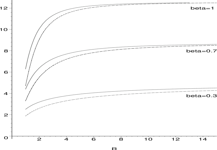
Figure 2: Displays the energies (in units of $J$-parameter) associated to $I$ and $P$ solitons, $E_{I}$ and $E_{P}$, represented by dashed and solid lines respectively. Note that as the cone is tighten, both energies appear to decrease in a such a way that the gap between $E_{I}$ and $E_{P}$ becomes greater, keeping always the more fundamental characteristic of $I$-type excitations. Here, we have taken $a=1$ and $c_{1}=0.1$.

Actually, in the preceding analysis we have considered that the nonmagnetic impurity is located at the soliton center, say, $\vec{\rho}=(0,0)$ (the apex of the cone). However, following the work presented in Ref.[8], we may wonder whether the effective potential between them would behave as long as they were placed one apart other. The way to perform that is analogous to that presented in Ref.[8], and we shall not repeat them here (we refer reader to such a reference for further details). After some calculation, we get (the soliton is centered at the apex, $\vec{\rho}=(0,0)=\vec{r}$):

$$\hskip-19.91684ptU_{\rm eff}=E_{0}\,\left\{\left[\frac{R^{2\beta}a^{\beta}(r_{0}^{\beta}-a^{\beta})^{2}}{\sqrt{(r_{0}^{\beta}-a^{\beta})^{2}+r_{0}^{2\beta}}[(r_{0}^{\beta}-a^{\beta})^{4}-R^{4\beta}]}-\frac{R^{2\beta}a^{\beta}(r_{0}^{\beta}+a^{\beta})^{2}}{\sqrt{(r_{0}^{\beta}+a^{\beta})^{2}+r_{0}^{2\beta}}[(r_{0}^{\beta}+a^{\beta})^{4}-R^{4\beta}]}\right]+\right.$$

$$\hskip 284.52756pt\left.-\frac{1}{4}\left(\frac{(Ra)^{\beta}}{(r_{0}^{2\beta}+R^{2\beta})}\right)^{2}\right\}\,,$$ (17)

where $\rho_{I}=r_{0}^{\beta}/\beta$ labels the impurity position. Notice that the singular points of $U_{\rm eff}$ appear at $(r_{0})^{\mp}_{S}=(R^{\beta}\mp\,a^{\beta})^{1/\beta}$. For example, if $\beta=1$ and $R=5a$, we then have $(r_{0})^{-}_{S}=4a$ and $(r_{0})^{+}_{S}=6a$. In Figure (3) we plot $U_{\rm eff}$ versus $r_{0}$ for some values of $\beta$. In general, the potential is attractive for $r_{0}<(R^{\beta}-\,a^{\beta})^{1/\beta}$ while for separation $r_{0}>(R^{\beta}+\,a^{\beta})^{1/\beta}$ its appears to be repulsive. Such a behavior was already obtained in the work of Ref.[8], for the planar, say, $\beta=1$ case.

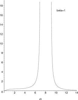
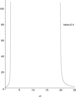
Figure 3: Exhibits the behavior of $U_{\rm eff}$ (in units of $J$-parameter) as function of the separation soliton-vacancy, $r_{0}$ (above $R=8a$ and $a=1$). Note that for short distances the potential is attractive while for large separations it turns out to be repulsive. Notice also that such an attractive interval decreases as $\beta$ gets lower values, indicating a stronger confinement (pinning) of the soliton whenever $\beta$ is sufficiently small. From left to right, we have $\beta=1,\,0.7,\,{\rm and}\,0.4$, respectively.

What our results bring as novelty is the fact that as long as the cone is tighten ($\beta$ gets lower) then the range of the attractive potential gets shorter. As a consequence, if we fix $R=5a$, and extrapolate our results to the discrete lattice (with spacing $a$), we conclude that for $\beta<\beta_{\rm cr}$ ($\beta_{\rm cr}=\ln(2)/\ln(5)\approx 0.43$, in this case), we get $r_{0}<a$ what implies that or the soliton is pinned on the impurity or they are quite apart one from another thanks to the repulsive potential. On the other hand, keeping the $R$-value above, whenever $\beta_{\rm cr}<\beta\leq 1$, we have the possibility of oscillating solitons around the spin-vacancy. Actually, let us take $U_{\rm eff}$ above, and consider small displacements impurity-soliton ($r_{0}$). Expanding it like below:

$$U_{\rm eff}|_{r_{0}\to 0}=E_{j}+\frac{1}{2}r_{0}^{2}\left(\frac{d^{2}U_{\rm eff}}{dr_{0}^{2}}\right)_{r_{0}=0}+\frac{1}{3}r_{0}^{3}\left(\frac{d^{3}U_{\rm eff}}{dr_{0}^{3}}\right)_{r_{0}=0}+\dots\,,$$ (18)

where we have taken into account the type of the excitation, according to (15-16). Now, looking only for the harmonic potential (say, the quadractic term) it is easy to show (we refer the reader to Ref.[10] for details) that the solitons oscillate around the spin vacancy with frequencies given by:

$$\omega_{j}=\sqrt{2}\frac{c}{a}\left[\frac{a_{j}^{2\beta}}{R^{2\beta}}+(R^{2\beta}+a_{j}^{2\beta})\left(\frac{a^{2\beta}}{\sqrt{5}[R^{4\beta}-(2a)^{4\beta}]}-\frac{a^{2\beta}}{4(R^{2\beta}+a^{2\beta})^{2}}\,,\right)\right]^{1/2}$$ (19)

where $a_{j}=a_{I},a_{P}$ ($a_{I}=1.01a$ and $a_{P}=0.23a$, see Ref.[6], for details) while $c=2JSa/\hbar=\sqrt{E_{j}/M_{j}}$, where $M_{j}$ is the soliton rest mass (for details, see Ref.[19]).

How $\omega_{j}$ behaves as function of the type ($I$ or $P$) and soliton size, $R$, for some values of $\beta$-parameter is shown in Figure (4). As expected, and earlier reported in Ref.[10], as soliton becomes larger, their frequency modes decrease. In addition, $I$-solitons oscillate faster than $P$-type ones. The novelty brought about here is that, as conical support is tighten the excitations appear to oscillate faster. In addition, notice also that for a given $\beta$ the soliton size should be $R>2^{1/\beta}a$ (in the discrete lattice). Thus, we see that for $\beta=1$ we should have $R\geq 3a$ while for $\beta=1/2$ such a radius should take values $\geq 5a$. However, despite such a size increasing, the geometry of the support deeply affects frequencies, as displayed in Figure (4).

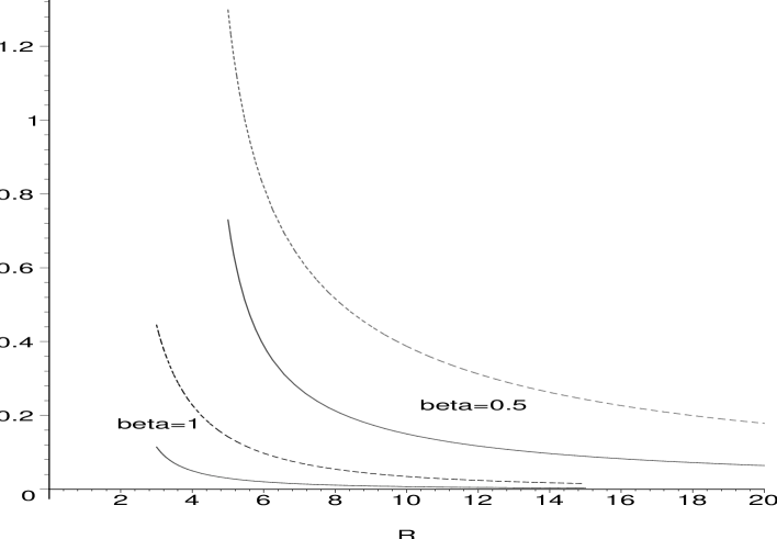
Figure 4: Shows solitonic frequencies, $\omega_{j}$ (in units of $c/a$), around the static impurity as function of soliton radius, $R$ (here $a=1$). Notice that $I$-excitations (dashed lines) present higher frequencies than $P$ ones (solid lines). Furthermore, note that as long as the cone is tighten, these excitations oscillate faster (the two lower curves are concerned to $\beta=1$ while the upper ones are related to $\beta=0.5$ ).

3 The Zeeman coupling and the instability of static solitonic solutions

In this section, we shall briefly discuss how the coupling of spins to an external magnetic field yields unstable static spin textures. Introducing the term $(\mu g\vec{B}\cdot\vec{n})\,V(\vec{\rho})=\mu\,gB_{0}\,m\,V(\vec{\rho})$ into Hamiltonian (1), where $\vec{B}=B_{0}\hat{z}$ ($B_{0}$ is homogeneous), the counterparts of dynamical equations (5,6) read like follows:

$$\hskip-22.76228pt\frac{\partial\,m}{\partial\,t}=V_{I}(\vec{\rho})\left[\nabla^{2}\Phi-\frac{2m}{(1-m^{2})}(\nabla m)\cdot(\nabla\Phi)\right]-\nabla\Phi\cdot\nabla V_{I}(\vec{\rho})\,,$$ (20)

$$\hskip-39.83368pt\frac{\partial\,\Phi}{\partial\,t}=V_{I}(\vec{\rho})\left[\nabla^{2}m+\frac{m}{(1-m^{2})}(\nabla m)^{2}+m(1-m^{2})(\nabla\Phi)^{2}-\xi_{B}^{-2}(1-m^{2})\right]-\nabla m\cdot\nabla V_{I}\,,$$ (21)

where $\xi_{B}^{2}=J/g\mu\,B_{0}$ is the magnetic length.

As we have done in the preceding case, supposing that $J>>g\mu\,B_{0}$ (spin-spin coupling is much stronger than Zeeman interaction) then, we have that eq. (9) is still valid here, while (10) is modified by the magnetic field. With the same assumptions taken in the preceding analysis (impurity at the soliton center, cylindrically symmetric solutions, etc), we conclude that $\Phi_{1}={\rm constant}$ remains the solution for its respective differential equation also here. However, eq. (11) now gets the form (using $m_{1}=m_{1}(m_{0})=m_{1}(u)$ analogously to eq. (11)):

$$\frac{d^{2}\,m_{1}}{du^{2}}+\frac{2\,m_{1}}{(1-u^{2})}=-\left(\frac{R}{\beta\xi_{B}}\right)^{2}\frac{(1-u^{2})^{\frac{1-\beta}{\beta}}}{(1-u)^{2/\beta}}\,.$$ (22)

Contrary to eq. (11), the above one does not present analytical closed solutions for arbitrary $\beta$, as far as we have tried. Indeed, by using MAPLE8 we have obatined closed expressions for some $\beta=1/N$-values ($N$ positive integer). Namely, we have noted that such expressions becomes more complicated as $N$ is rised. By virtue of their length, we shall not write them here. Rather, in Figure (5) we plot $m=m_{0}+m_{1}$ as function of distance, $r$. The main point to be noticed here is that no good $m_{1}$-functions solves eq. (22), what may be realized by noting that $m$ blows up as $r\to\infty$, yielding divergent associated energy. Actually, in the very beginning we have defined $m=\cos(\theta)$, but the results plotted in Figure (5) explicitly shows us that for $r>L_{c}$ (depending upon $\beta$) $m$-variable takes values $>1$, what is a contradiction. Thus, we conclude that whenever Zeeman corrections are taken on $m$ solitonic profile these excitations appear to get unstable and collapse. Furthermore, once that such a blowing up character of $m$-profile comes about by turning on $\vec{B}$-field and appear to become stronger as long as the cone aperture gets smaller, we may realize that by decreasing $\beta$-parameter we can increase the net magnetic effect on solitonic excitations. Such a result can be viewed as a geometrical accentuation of the magnetic field experienced by solitons.

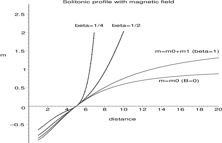
Figure 5: Displays $m$ solitonic profile versus distance, $r$. Without external magnetic field, $m=m_{0}$ and $m\to 1$ as $r\to\infty$. However, whenever $\vec{B}$ is turned on, such a profile present values $>1$ for $r>L_{c}$, what contradicts $m$ definition and implies that static solitons becomes unstable. In addition, note that such a critical size, $L_{c}$ gets smaller values as $\beta$ is lowered.

Notice, however, that we cannot state that they shrink to point-like objects, since the impurity introduces a characteristic length and no smaller size than spin vacancy is possible (recall that the impurity was placed at soliton center). In the discrete lattice case, we would expect that Zeeman interaction should force solitons to shrink to the smallest size: the lattice spacing $a$. Notice, however, that this is pointed out here as a possibility (following the conclusions presented in Refs.[13, 14]) once our analysis is strictly valid only for $r>a$. Indeed, a similar problem was earlier considered in the work of Ref.[14]. There, the authors explicitly state the impossibility of carrying out their analytical analysis for the highly complicated diferential equations.

Even though we could not provide here a rigorous proof of whether the solitons necessarily decreases their radius to spin vacancy size in order to compensate the instability brought about by Zeeman interaction, we should mention that the present problem is important in connection with dynamical solitons, for instance, in the lines of Ref.[20]. Thus, considering precessional oscillatory modes of a soliton around $\vec{B}$, their associated frequencies could be determined and how geometrical features affect such modes. Such an issue is under investigation and results will be communicated elsewhere[21].

4 Conclusions and Prospects

We have considered the problem of classical Heisenberg spins on a circular conical geometry subject to both the potential of a static non-magnetic impurity and an external magnetic field. Whenever spins weekly interact with the impurity alone, a number of results were obtained and compared to their planar counterparts. In general, our results recover planar ones as long as $\beta=1$, and for arbitrary cone aperture they describe how solitonic spin textures are affected by a static spin vacancy in such a geometry. Among other, we have seen that the impurity presence now allows the appearance of two kinds of solitons: $I$ and $P$-type ones. In this line, one interesting thing realized in conical geometry is that the energies of both types get smaller values whenever the cone is tighten while the energy gap between them is increased. Since both kinds of excitations have been recently observed in experiments, we could think of similar experiments dealing with Heisenberg-like spins on conical supports in order to determine the results predicted here.

Since NL$\sigma$ model has been also applied to study weekly self-interacting two-dimensional electron gas (2DEG) [22], our present study may also be relevant, for instance, in connection with Quantum Hall Effect in curved, say, conical, geometry.

An analysis of how external magnetic field influences the structure of dynamical solitons is in order. For instance, how their internal precessional modes and sizes are influenced by this field are some of the issues we have been addressing. Results concerning such a study will be communicated elsewhere[21].

As prospects for future investigation, we may quote the introduction of more impurities in the system, for example, as presented in the works of Refs.[11, 23]. There, analytical and numerical/simulational analysis of the model may indicate how collective spin vacancies effects are read by solitonic excitations.

Concerned with the current topic of magnetic nanostructured objects, how nanomagnetic cones [17, 18] (among other curved structures), with and without vacancies and magnetic field, affects the magnetization and hysteresis loops are some interesting points to be studied.

Finally, in connection with Field Theory/High Energy Physics and related topics, a problem that could lead to interesting results is that of a charged particle interacting with a magnetic monopole in a conical background. Perhaps, in this framework, bound states between them could be observed, scenario quite distinct from its flat space counterpart, which does not present closed orbit configurations between the m [24].

Acknowledgments

WAF and ARP thank CNPq for financial support. WAM-M acknowlegdes FAPEMIG for partial financial support.

References

-
[1]
S. Chakravarty, B.I. Halperin, D.R. Nelson, Phys. Rev. Lett.
60 (1988) 1057; Phys. Rev. B39 (1989) 2344;
E. Manousakis, Rev. Mod. Phys. 63 (1991) 1;
D.J. Thouless, Topological Quantum Numbers in Non-relativistic Physics, World Scientific Publishing, 1998;
D.R. Nelson, Defects and Geometry in Condensed Matter Physics, (Cambridge Univ. Press, 2002). - [2] A.A. Belavin and A.M. Polyakov, JETP Lett. 22 (1975) 245.
- [3] L. Ryder, ”Quantum Field Theory”, 2nd edition, Cambridge Univ. Press, 1996.
-
[4]
V. Berezinskii, Sov. Phys., JETP 32 (1970) 493;
J.M. Kosterlitz and D.J. Thouless, J. Phys. C6 (1973) 1181. -
[5]
M.-H. Julien, T. Fehér, M. Horvatić, C. Berthier, O.N.
Bakharev, P. Ségransan, G. Collin, and J.-F. Marucco, Phys. Rev. Lett.
84 (2000) 3422;
J. Bobroff, H. Alloul, W.A. MacFarlane, P. Mendels, N. Blanchard, G. Collin, and J.-F. Marucco, Phys. Rev. Lett. 86 (2001) 4116. - [6] K. Subbaraman, C.E. Zaspel, and J.E. Drumheller, Phys. Rev. Lett. 80 (1998) 2201.
- [7] C.E. Zaspel, J.E. Drumheller, and K. Subbaraman, Phys. Stat. Sol. A189 (2202)1029.
- [8] A.R. Pereira and A.S.T. Pires, J. Mag. Mag. Mat. 257 (2003) 290.
- [9] L.A.S. Mól, A.R. Pereira, and A.S.T. Pires, Phys. Rev. B66 (2002) 052415.
- [10] L.A.S. Mól, A.R. Pereira, and W.A. Moura-Melo, Phys. Rev. B67 (2003) 132403.
- [11] S.A. Leonel, P.Z. Coura, A.R. Pereira, L.A.S. Mól, and B.V. Costa, Phys. Rev. B67 (2003) 104426.
- [12] A.R. Pereira, Phys. Lett. A314 (2003) 102.
-
[13]
S. Villain-Guillot, R. Dandoloff, and A. Saxena, Phys.
Lett. A188 (1994) 343;
R. Dandoloff, S. Villain-Guillot, A. Saxena, and A.R. Bishop, Phys. Rev. Lett. 74 (1995) 813;
A. Saxena and R. Dandoloff, Phys. Rev. B55 (1997) 11049;
R. Dandoloff and A. Saxena, Eur. Phys. J. B29 (2002) 265. - [14] A. Saxena and R. Dandoloff, Phys. Rev. B66 (2002) 104414.
- [15] A. Saxena, R. Dandoloff, and T. Lookman, Phys. A261 (1998) 13;
- [16] A.R. Pereira, ”Heisenberg spins on a circular conical surface”, J. Mag. Mag. Mat. (2004) doi:10.1016/j.jmmm.2004.07.015 in press.
-
[17]
B.A. Everitt, A.V. Pohm, and J.M.
Daughton, J. Appl. Phys. 81 (1997) 4020;
S.S.P. Parkin et al, J. Appl. Phys. 85 (1999) 5828;
S. Tehrani et al, IEEE Trans. Magn. 36 (2000) 2752;
R.P. Cowburn and M.E. Welland, Science 287 (2000) 1466;
C.A. Ross, Ann. Rev. Mater. Res. 31 (2001) 203. -
[18]
C.A. Ross et at, J. Appl. Phys. 89 (2001)
1310;
C.A. Ross et al, J. Appl. Phys. 91 (2002) 6848;
A.R. Pereira, “Inhomogeneous states in permalloy nanodisks with point defects” [submitted to Phys. Rev. B (2004)]. -
[19]
G.M. Wysin, Phys. Rev. B63 (2001) 094402;
A.R. Pereira and A.S.T. Pires, Phys. Rev. B51 (1995) 996. -
[20]
F.K. Abdullaev, R.M. Galimzyanov, and A.S. Kirakosyan,
Phys. Rev. B60 (1999) 6552;
D.D Sheka, B.A. Ivanov, F.G. Mertens, Phys. Rev. 64 (2001) 24432;
G.M. Rocha-Filho and A.R. Pereira, Sol. State Comm. 122 (2002) 83. - [21] W.A. Freitas, W.A. Moura-Melo and A.R. Pereira, work in progress.
- [22] S.L. Sondhi, A. Karlherde, S.A. Kivelson, and E.H. Rezayi, Phys. Rev. B47 (1993) 16419.
- [23] F.M. Paula, A.R. Pereira and L.A.S. Mól, Phys. Lett. A329 (2004) 155.
- [24] P.A.M. Dirac, Proc. Royal Soc. [London] A133 (1931) 60.