Aperiodic quantum XXZ chains: Renormalization-group results

Abstract

We report a comprehensive investigation of the low-energy properties of antiferromagnetic quantum XXZ spin chains with aperiodic couplings. We use an adaptation of the Ma-Dasgupta-Hu renormalization-group method to obtain analytical and numerical results for the low-temperature thermodynamics and the ground-state correlations of chains with couplings following several two-letter aperiodic sequences, including the quasiperiodic Fibonacci and other precious-mean sequences, as well as sequences inducing strong geometrical fluctuations. For a given aperiodic sequence, we argue that in the easy-plane anisotropy regime, intermediate between the XX and Heisenberg limits, the general scaling form of the thermodynamic properties is essentially given by the exactly-known XX behavior, providing a classification of the effects of aperiodicity on XXZ chains. We also discuss the nature of the ground-state structures, and their comparison with the random-singlet phase, characteristic of random-bond chains.

I Introduction

At low temperatures, the interplay between lack of translational invariance and quantum fluctuations in low-dimensional strongly-correlated electron systems may induce novel phases with peculiar behavior. In particular, randomness in quantum spin chains may lead to Griffiths phases,Fisher (1992, 1995) random quantum paramagnetism,Furusaki et al. (1994, 1995); Nguyen et al. (1996) large-spin formation,Westerberg et al. (1995, 1997) and random-singlet phases.Fisher (1994); Refael et al. (2002) On the other hand, studies on the influence of deterministic but aperiodic elements on similar systems (see e.g. Refs. Kohmoto et al., 1983; Luck and Nieuwenhuizen, 1986; Luck, 1993a; Vidal et al., 1999, 2001; Hida, 1999, 2001; Hermisson, 2000; Arlego et al., 2001), inspired by the experimental discovery of quasicrystals,Shechtman et al. (1984) have revealed strong effects on dynamical and thermodynamic properties, although much less is known concerning the precise nature of the underlying ground-state phases.

Prototypical models for those studies are spin-$\nicefrac{{1}}{{2}}$ antiferromagnetic XXZ chains described by the Hamiltonian

$$H=\sum_{i}J_{i}\left(S_{i}^{x}S_{i+1}^{x}+S_{i}^{y}S_{i+1}^{y}+\Delta S_{i}^{z}S_{i+1}^{z}\right),$$ (1)

where $J_{i}>0$ and the $S_{i}$ are spin operators. In the uniform case ($J_{i}\equiv J$), the ground state for chains with $-1<\Delta\leq 1$ is critical,Baxter (1972) exhibiting power-law decay of the pair correlations as a function of the distance between spins,Luther and Peschel (1975) as well as gapless elementary excitations. Such critical phase is unstable towards dimerization, i.e. the introduction of alternating couplings $J_{\mathrm{{odd}}}$ and $J_{\mathrm{{even}}}$, in the presence of which a gap opens between the (now localized) ground state and the first excitated states.Cross and Fisher (1979); Bonner and Blöte (1982); Barnes et al. (1999) This instability hints at the profound effects produced by fully breaking the translational symmetry of the system.

Random-bond versions of these chains have been much studied by a real-space renormalization-group (RG) method introducedMa et al. (1979); Dasgupta and Ma (1980) by Ma, Dasgupta and Hu (MDH) for the Heisenberg chain ($\Delta=1$) and more recently extended by Fisher,Fisher (1992, 1994, 1995) who gave evidence that the method becomes asymptotically exact at low energies. In the last few years, the method has been applied and adapted to a variety of random systems (see e.g. Refs. Westerberg et al., 1995, 1997; Hyman et al., 1996; Le Doussal et al., 1999; Saguia et al., 2002; Yusuf and Yang, 2002; Hoyos and Miranda, 2004a; Hooyberghs et al., 2003; Hoyos and Miranda, 2004b). The basic idea is to decimate the spin pairs coupled by the strongest bonds (those with the largest gaps between the local ground state and the first excited multiplet), forming singlets and inducing weak effective couplings between neighboring spins, thereby reducing the energy scale. For XXZ chains in the regime $-\nicefrac{{1}}{{2}}<\Delta\leq 1$, the method predicts the ground state to be a random-singlet phase, consisting of arbitrarily distant spins forming rare, strongly-correlated singlet pairs.Fisher (1994)

Another way of breaking the translational symmetry is suggested by analogies with quasicrystals. These are structures which exhibit symmetries forbidden by traditional crystalography, and which correspond to projections of higher-dimensional Bravais lattices onto low-dimensional subspaces.Janner and Janssen (1977) A one-dimensional example is provided by the Fibonacci quasiperiodic chain, obtained from a cut-and-project operation on a square lattice.Elser (1985) In this chain, spins are separated by two possible distances, $a$ and $b$, whose sequence, starting from the left end of the chain, is $abaab\ldots$ This sequence can be generated by repeatedly applying a substitution (or inflation) rule $a\rightarrow ab$, $b\rightarrow a$, starting from a single distance $a$. Associating with each $a$ a coupling $J_{a}$ and with each $b$ a coupling $J_{b}$ we obtain a spin chain with couplings following a Fibonacci sequence. More generally, we can postulate a two-letter substitution rule, build the corresponding letter sequence, and associate couplings with letters to obtain spin chains whose couplings follow aperiodic but deterministic sequences. Quasiperiodic sequences are characterized by a Fourier spectrum consisting of Bragg peaks, but more complex spectra (such as singular continuous) can be generated by substitution rules.Godrèche and Luck (1992) In this work we apply the term ‘aperiodic’ when referring to nonperiodic, self-similar sequences, also encompassing those which are strictly quasiperiodic in the above sense.

In XX spin chains ($\Delta=0$), the low-temperature thermodynamic behavior can be qualitatively determined for virtually any aperiodic sequence by an exact RG method.Hermisson (2000) The effects of aperiodicity depend on topological properties of the sequence. If the fraction of letters $a$ (or $b$) at odd positions is different from that at even positions (i.e. if there is average dimerization), then a finite gap opens between the global ground state and the first excited states, and the chain becomes noncritical. Otherwise, the scaling of the lowest gaps can be classified according to the wandering exponent $\omega$ measuring the geometric fluctuations $g$ related to nonoverlapping pairs of letters,Hermisson (2000) which vary with the system size $N$ as $g\sim N^{\omega}$. If $\omega<0$, aperiodicity has no effect on the long-distance, low-temperature properties, and the system behaves as in the uniform case, with a finite susceptibility at $T=0$. If $\omega=0$, as in the Fibonacci sequence, aperiodicity is marginal and may lead to nonuniversal power-law scaling behavior of thermodynamic properties. If $\omega>0$, aperiodicity is relevant in the RG sense, affecting the $T=0$ critical behavior and leading to exponential scaling of the lowest gaps $\Lambda$ at long distances $r$, according to the form $\Lambda\sim\exp\left(-r^{\omega}\right)$. In particular, for sequences with $\omega=\nicefrac{{1}}{{2}}$, geometric fluctuations mimic those induced by randomness, and the scaling behavior is similar to the one characterizing the random-singlet phase.Fisher (1994)

In contrast, results for the effects of aperiodicity on low-energy properties of XXZ chains have been so far scarce, and restricted to particular sequences. Vidal, Mouhanna and GiamarchiVidal et al. (1999, 2001) studied the related problem of an interacting spinless fermion chain with Fibonacci or precious-mean potential by using bosonization techniques, which are valid in the weak-modulation regime ($J_{a}\simeq J_{b}$). At half filling, where the system corresponds to an XXZ chain in zero external field, their calculations predict that aperiodicity will drive the system away from the usual Luttinger-liquid behavior for $0\leq\Delta\leq 1$. A similar conclusion is drawn from studies on a Hubbard chain with hoppings following a Fibonacci sequence.Hida (2001) Density-matrix renormalization-group (DMRG) results on XXZ chains with precious-mean couplings,Hida (1999) and recent real-space RG calculations on the Fibonacci XXZ chainHida (2004a, b) (also based on the MDH scheme), likewise predict that low-temperature properties are different than in the uniform chains. The zero-temperature magnetization curve of Fibonacci XXZ chains has also been investigated,Arlego et al. (2001) with emphasis on determining the plateau structure.

Our aim in this paper is to investigate the effects of arbitrary aperiodic coupling distributions on the low-temperature properties of XXZ chains, reinforcing and extending our previous results.Vieira From an adaptation of the Ma-Dasgupta-Hu RG scheme, we obtain information about low-temperature thermodynamics and ground-state correlation functions for several aperiodic sequences. Our results, which are presumably exact in the strong-modulation limit ($J_{a}\ll J_{b}$ or $J_{a}\gg J_{b}$), point to the following conclusions:

• The exact classification found in the XX limit can arguably be extended to XXZ chains in the anisotropy regime $0<\Delta\leq 1$. We predict that dimerized aperiodicity opens a gap to the lowest excitations, and that otherwise the effects of aperiodicity on the low-temperature thermodynamics are gauged by the same exponent $\omega$, irrespective of anisotropy. In particular, sequences which are strictly marginal in the XX limit continue to be so for anisotropies $0<\Delta<1$, but may be marginally relevant in the Heisenberg limit.

• On the other hand, $\omega$ is found not to define the behavior of correlation functions, although ground-state structures in the presence of marginal or relevant couplings also reflect self-similar properties of the sequences. Dominant correlations correspond to well-defined distances, related to the rescaling factor of the sequences (contrary to the random-singlet phase, where no such characteristic distances exist), and two types of behavior are possible: either the chains can be decomposed into a hierarchy of singlets, forming a kind of ‘aperiodic-singlet phase’, or into a hierarchy of effective spins, in which case low-energy excitations involve an exponentially large number of spins. This is in sharp contrast both to the gapless spin-wave excitations of the uniform chains and to the gapped triplet-wave excitations of the dimerized chains.

• Based on second-order calculations, the long-distance decay exponents of average ground-state correlation functions are seen to vary with the coupling ratio in the presence of strictly marginal aperiodicity. Otherwise, strong universality (i.e. independence of the exponents on both coupling ratio and anisotropy) is obtained for the whole line $0\leq\Delta<1$, although different decay exponents may emerge in the Heisenberg limit. Also, the scaling form of typical (rather than average) correlations follows essentially the same scaling form as the energy gaps, similarly to what happens for random-bond chains.

In order to make the paper self-contained, we begin by reviewing some known results. So, in Sec. II we present the basics of the Ma-Dasgupta-Hu scheme, as applied to random-bond XXZ chains, and summarize the properties of the underlying random-singlet phase. Also, in Sec. III we provide a short discussion on aperiodic sequences, as well as a sketch of the exact RG results for XX chains with aperiodic couplings. Our adaptation of the Ma-Dasgupta-Hu method to aperiodic XXZ chains is described in Sec. IV, and results for marginal and relevant aperiodicity are presented in Secs. V and VI. The final section is devoted to a discussion and conclusions. There are also two appendices, in which some important technical points are detailed.

II Random-bond spin chains and the Ma-Dasgupta-Hu method

Consider an antiferromagnetic quantum spin-$\nicefrac{{1}}{{2}}$ chain described by the Hamiltonian

$$H=\sum_{i}J_{i}\left(S_{i}^{x}S_{i+1}^{x}+S_{i}^{y}S_{i+1}^{y}+\Delta_{i}S_{i}^{z}S_{i+1}^{z}\right),$$ (2)

where $J_{i}>0$ and all anisotropies are such that $0\leq\Delta_{i}\leq 1$. Let us assume that the couplings $J_{i}$ are randomly distributed according to a broad probability distribution $\wp(J_{i})$ having an upper cutoff $J_{\textrm{max}}$. Under such conditions, in a finite but large chain, there is a strongest bond $J_{0}\simeq J_{\textrm{max}}$ connecting, say, spins $S_{1}$ and $S_{2}$, which on their turn are coupled to their other nearest neighbors $S_{l}$ and $S_{r}$ by weaker bonds $J_{l}$ and $J_{r}$. The local Hamiltonian connecting $S_{1}$ and $S_{2}$ is

$$H_{0}=J_{0}\left(S_{1}^{x}S_{2}^{x}+S_{1}^{y}S_{2}^{y}+\Delta_{0}S_{1}^{z}S_{2}^{z}\right),$$

whose ground state is a singlet, separated from the first excited states by an energy gap $\Lambda_{0}=\tfrac{1}{2}(1+\Delta_{0})J_{0}$. The idea behind the Ma-Dasgupta-HuMa et al. (1979); Dasgupta and Ma (1980) method is that, at temperatures below $\Lambda_{0}$, $S_{1}$ and $S_{2}$ can be decimated out of the system, since they couple into a singlet, giving a negligible contribution to thermodynamic properties. Nevertheless, their virtual excitations induce a weak effective coupling between $S_{l}$ and $S_{r}$, described by the Hamiltonian

$$H^{\prime}=J^{\prime}\left(S_{l}^{x}S_{r}^{x}+S_{l}^{y}S_{r}^{y}+\Delta^{\prime}S_{l}^{z}S_{r}^{z}\right).$$

The parameters $J^{\prime}$ and $\Delta^{\prime}$ can be obtained by second-order perturbation theory (see Appendix A), and are given by

$$J^{\prime}=\frac{1}{1+\Delta_{0}}\cdot\frac{J_{l}J_{r}}{J_{0}}\quad\textrm{and}\quad\Delta^{\prime}=\frac{1+\Delta_{0}}{2}\Delta_{l}\Delta_{r}.$$ (3)

Notice that $J^{\prime}$ is smaller than either $J_{l}$, $J_{r}$ or $J_{0}$; likewise, unless all $\Delta_{i}=1$, $\Delta^{\prime}$ is smaller than either $\Delta_{l}$ or $\Delta_{r}$. Thus, after eliminating $S_{1}$ and $S_{2}$, the overall energy scale is reduced. The previous steps can be repeated with the next largest bond, which most probably is not $J^{\prime}$.

Starting from Eqs. (3), FisherFisher (1994) was able to write and solve recursion relations for the probability distribution of the effective couplings. The fixed-point distribution is presumably independent of the initial couplings,Laflorencie and Rieger (2003) and diverges as a power law for $J^{\prime}\to 0^{+}$, indicating that the perturbative approach leading to Eqs. (3) becomes essentially exact for asymptotically low energies.

The ground state is a ‘random-singlet’ phase, consisting of arbitrarily distant spins forming rare, strongly correlated singlet pairs.Doty and Fisher (1992); Fisher (1994) Exciting a singlet whose spins are separated by a distance $r$ costs an energy of order $\Lambda$, with a dynamic scaling form

$$\Lambda\sim e^{-\mu\sqrt{r/r_{0}}},$$

where $\mu$ and $r_{0}$ are constants. At low temperatures, the zero-field susceptibility diverges as

$$\chi\sim\frac{1}{T\ln^{2}T}.$$

Average ground-state correlations are dominated by the rare singlet pairs, and decay as a power law,

$$C(r)\equiv\left|\overline{\left\langle\mathbf{S}_{i}\cdot\mathbf{S}_{i+r}\right\rangle}\right|\sim\frac{1}{r^{2}},$$

where the bar denotes average over the whole chain, while typical correlations are short-ranged, following

$$C_{\mathrm{typ}}(r)\sim e^{-\mu_{\mathrm{typ}}\sqrt{r/r_{0}}}.$$

These asymptotic results are independent of the anisotropies $\Delta_{i}$, as long as $0\leq\Delta_{i}\leq 1$ for all $i$, with the same distribution on even and odd bonds.

III Aperiodic sequences and XX chains

Following closely the analysis of Hermisson,Hermisson (2000) in this Section we consider antiferromagnetic quantum XX chains, described by the Hamiltonian

$$H=\sum_{i}J_{i}\left(S_{i}^{x}S_{i+1}^{x}+S_{i}^{y}S_{i+1}^{y}\right),$$ (4)

where now the strengths of the site-dependent couplings $J_{i}$ can be either $J_{a}$ or $J_{b}$, and are distributed according to deterministic but aperiodic binary sequences, obtained by substitution (or inflation) rules of the form

$$\sigma:\ \left\{\begin{array}[]{c}a\to w_{a}\\ b\to w_{b}\end{array}\right.,$$

where $w_{a}$ and $w_{b}$ are words (finite strings) composed of letters $a$ and $b$. A well-know example is provided by the Fibonacci sequence, whose substitution rule is

$$\sigma_{\textrm{fb}}:\left\{\begin{array}[]{l}a\to ab\\ b\to a\end{array}\right..$$

Starting from a single letter $a$, repeated application of $\sigma_{\textrm{fb}}$ yields strings with lengths given by the Fibonacci numbers $1$, $2$, $3$, $5$, $8$,$\ldots$, ultimately producing a letter sequence $abaababaaba\ldots$, for which no period can be identified.

Given an inflation rule $\sigma$, various statistical propertiesQuefféllec (1987) of the associated sequence are enclosed in the substitution matrix

$$\mathbf{M}=\left(\begin{array}[]{cc}\#_{a}(w_{a})&\#_{a}(w_{b})\\ \#_{b}(w_{a})&\#_{b}(w_{b})\end{array}\right),$$

where $\#_{a}(w_{b})$ denotes the number of letters $a$ in the word $w_{b}$. The largest eigenvalue of $\mathbf{M}$, $\lambda_{+}$, gives the asymptotic scaling factor of the string length (i.e. the ratio between the lengths of the strings corresponding to successive iterations of the rule $\sigma$); the entries of the corresponding eigenvector are proportional to the frequencies $p_{a}$ and $p_{b}$ of letters $a$ and $b$ in the limit (infinite) sequence.

The remaining eigenvalue, $\lambda_{-}$, is related to the geometric fluctuations of the sequence, which are defined in the following way. Let $N_{n}^{a}$ be the number of letters $a$ in the string obtained after $n$ iterations of $\sigma$, and $N_{n}$ be the corresponding total number of letters (the length of the string). Then, a measure of the geometric fluctuations induced by the sequence is the difference $g_{n}$ between $N_{n}^{a}$ and the number of letters $a$ expected from the limit-sequence frequency $p_{a}$, and this behaves as

$$g_{n}=\left|N_{n}^{a}-p_{a}N_{n}\right|\sim\left|\lambda_{-}\right|^{n}.$$

Since $N_{n}\sim\lambda_{+}^{n}$, this last equation can be rewritten as

$$g_{n}\sim N_{n}^{\omega_{l}},$$

by defining the ‘wandering exponent’

$$\omega_{l}=\frac{\ln\left|\lambda_{-}\right|}{\ln\lambda_{+}}.$$

If $\omega_{l}<0$, fluctuations become smaller as the string grows, and the sequence looks more and more ‘periodic’. On the other hand, if $\omega_{l}>0$, fluctuations increase without limit. The marginal case $\omega_{l}=0$ is in general connected to logarithmic fluctuations. It can be shownLuck et al. (1993) that substitutions for which $\omega_{l}<0$ generate quasiperiodic (or limit-quasiperiodic) sequences.

The concept of geometric fluctuations is essential in establishing the Harris-Luck criterionHarris (1974); Luck (1993b) for the relevance of inhomogeneities to the critical behavior of magnetic systems. The criterion states that, if fluctuations in the local parameters controlling the criticality of the system vary with some characteristic length $L$ as $g\sim L^{\omega}$, then there is a critical value of the exponent $\omega$ above which the presence of inhomogeneities can affect the critical behavior. This happens for

$$\omega>1-\frac{1}{d\nu},$$ (5)

where $d$ is the number of dimensions along which inhomogeneities are distributed, and $\nu$ is the correlation-length critical exponent of the underlying uniform system. Randomly distributed inhomogeneities lead to $\omega=\nicefrac{{1}}{{2}}$, and the general Harris criterionHarris (1974); Lubensky (1975); Muzy et al. (2002) is recovered.

The ground-state of the model in Eq. (4) is critical in the uniform limit ($J_{i}\equiv J$): there is no energy gap to the low-lying excitations, and pair correlations decay as power laws,Lieb et al. (1961)

$$C^{\alpha\alpha}(r)=\left|\overline{\left\langle S_{i}^{\alpha}S_{i+r}^{\alpha}\right\rangle}\right|\sim r^{-\eta^{\alpha\alpha}},$$

with $\eta^{xx}=\eta^{yy}=\nicefrac{{1}}{{2}}$ and $\eta^{zz}=2$. This phase is unstable towards dimerization (i.e. the presence of couplings $J_{\textrm{o}}$ and $J_{\textrm{e}}$ alternating between odd and even bonds), in which case a gap opens in the low-energy spectrum, and ground-state correlations become short-ranged. More generally, the model exhibits a (zero-temperature) quantum phase transition between two dimer phases forPfeuty (1979); Hermisson (2000)

$$\delta=\overline{\ln J_{2j-1}}-\overline{\ln J_{2j}}=0.$$ (6)

If $J_{2j-1}\equiv J_{\textrm{o}}$ and $J_{2j}\equiv J_{\textrm{e}}$, the phase transition occurs for $\delta=\ln(J_{\textrm{o}}/J_{\textrm{e}})=0$, and belongs to the Onsager universality class, with $\nu=1$.

When the couplings $J_{i}$ are chosen according to aperiodic sequences for which the fractions of letters $a$ (or $b$) at even and odd positions are different, Eq. (6) is not satisfied, and the system is in a dimer phase. This suggests that the local parameters defining the criticality of XX chains are the shifts $\delta_{j}=\ln(J_{2j-1}/J_{2j})$. In order to study the fluctuations of the $\delta_{j}$, which depend on two consecutive couplings, we must usually consider the sequence of nonoverlapping letter pairs associated with a given aperiodic sequence. To build the inflation rule $\sigma^{(2)}$ for such pairs, it is necessary to iterate the original rule $\sigma$ until the strings obtained from a single $a$ and $b$ have lengths of the same parity. As an illustration, let us take the Fibonacci sequence. Applying $\sigma_{\textrm{fb}}$ three times yields

$$\sigma_{\textrm{fb}}^{3}:\left\{\begin{array}[]{l}a\to abaab\\ b\to aba\end{array}\right..$$

Noting that the pair $bb$ does not occur in the sequence, we readily obtain

$$\sigma_{\textrm{fb}}^{(2)}:\left\{\begin{array}[]{l}aa\to(ab)(aa)(ba)(ba)(ab)\\ ab\to(ab)(aa)(ba)(ba)\\ ba\to(ab)(aa)(ba)(ab)\end{array}\right..$$

For a general pair inflation rule $\sigma^{(2)}$, we can define an associated substitution matrix

$$\mathbf{M}^{(2)}=\left(\begin{array}[]{cccc}\#_{aa}(w_{aa})&\#_{aa}(w_{ab})&\#_{aa}(w_{ba})&\#_{aa}(w_{bb})\\ \#_{ab}(w_{aa})&\#_{ab}(w_{ab})&\#_{ab}(w_{ba})&\#_{ab}(w_{bb})\\ \#_{ba}(w_{aa})&\#_{ba}(w_{ab})&\#_{ba}(w_{ba})&\#_{ba}(w_{bb})\\ \#_{bb}(w_{aa})&\#_{bb}(w_{ab})&\#_{bb}(w_{ba})&\#_{bb}(w_{bb})\end{array}\right),$$

where now $\#_{ab}(w_{ba})$ denotes the number of pairs $ab$ in the word associated with the pair $ba$. The leading eigenvalues $\lambda_{1}$ and $\lambda_{2}$ of $\mathbf{M}^{(2)}$ define another wandering exponent

$$\omega=\frac{\ln\left|\lambda_{2}\right|}{\ln\lambda_{1}},$$

which governs the fluctuations of the letter pairs, and consequently of the $\delta_{j}$. It is essential to note that $\omega$ is in general different from $\omega_{l}$: for the Fibonacci sequence, for instance, we have $\omega_{l}=-1$, but $\omega=0$.

By an exact renormalization-group treatment, HermissonHermisson (2000) was able to build recursion relations for effective couplings, and to show that, in agreement with the above heuristic argument, the eigenvalues $\lambda_{i}$ of $\mathbf{M}^{(2)}$ give directly the RG eigenvalues $y_{i}$ around the uniform fixed point of XY chains with aperiodic couplings,

$$y_{i}=\frac{\ln\left|\lambda_{i}\right|}{\ln\lambda_{1}},$$

while the corresponding eigenvectors yield the scaling fields. Thus, aperiodicity is relevant in the RG sense (i.e. it moves the RG flows away from the uniform fixed point) if the next-to-leading eigenvalue $y_{2}=\omega$ is positive, exactly as predicted by the Harris-Luck criterion, Eq. (5), with $d=\nu=1$.

For a large class of aperiodic sequences fulfilling Eq. (6), $\lambda_{2}$ is given in the XX limit by an integer $k$. When a pair substitution rule can be defined, this integer is simply given by

$$k=\#_{ab}(w_{ab})-\#_{ba}(w_{ab}).$$

Thus, the wandering exponent in the XX limit is of the form

$$\omega=\frac{\ln k}{\ln\tau},$$ (7)

where $\tau\equiv\lambda_{1}$ corresponds to the rescaling factor of the sequence of letter pairs.

It is also possible to determine the scaling of the lowest energy levels $\Lambda$ with the system size $r$. For irrelevant or marginal aperiodicity ($\omega\leq 0$) we have

$$\Lambda\sim r^{-z},$$ (8)

with a dynamical exponent $z$ equal to unity if $\omega<0$, but which can vary with the coupling ratio $J_{a}/J_{b}$ in the marginal cases ($\omega=0$). Relevant aperiodicity ($\omega>0$) leads to a different scaling form,

$$\Lambda\sim\exp\left(-\mu r^{\omega}\right),\qquad(\mu=\textrm{constant})$$ (9)

and to a formally infinite dynamical exponent. From Eqs. (8) and (9), scaling forms for low-temperature thermodynamic properties such as the specific heat and zero-field susceptibility can be obtained, as discussed in the next sections. Ground-state correlation functions, however, do not seem to be simply accessible from the exact RG treatment.

Since the critical phase of uniform XXZ chains is also unstable towards dimerization in the whole anisotropy regime $0<\Delta\leq 1$, one might expect that the relevant geometrical fluctuations in the presence of aperiodic couplings would be somehow related to the $\delta_{j}$ defined above. Consequently, the exponent $\omega$ would be involved in determining the scaling behavior of thermodynamic properties of aperiodic chains for all anisotropies intermediate between the XX and Heisenberg limits. The results of the next sections indeed provide evidence that this seems to be the case.

IV The Ma-Dasgupta-Hu method for aperiodic XXZ chains

We now wish to investigate the effects of aperiodic couplings on XXZ chains described by the Hamiltonian in Eq. (2). Based on the success of the Ma-Dasgupta-Hu scheme in predicting the properties of random-bond chains, we expect that it also works in the presence of aperiodicity. We concentrate on the case of uniform anisotropy ($\Delta_{i}\equiv\Delta$), but more general situations can be considered.

Applying the MDH method to aperiodic chains requires taking into account that now, since we have only two distinct coupling constants, there are many spin blocks with the same (largest) gap at a given energy scale. Also, those blocks may consist of more than two spins, in which case effective spins would form upon renormalization. The strategy is to sweep through the lattice until all blocks with the same gap have been renormalized, leading to new effective couplings (and possibly spins). Then we search for the next largest gap, which again corresponds to many blocks. When all possible original blocks have been considered, there remains some unrenormalized spins, possibly along with effective ones, defining new blocks which form a second generation of the lattice. The process is then iterated, leading to the renormalization of the spatial distribution of effective blocks (or bonds) along the generations.

Due to the self-similarity inherent to aperiodic sequences generated by inflation rules, it is natural that the block distribution reaches a periodic attractor (usually a fixed point or a two-cycle) after a few lattice sweeps; numerical implementations of the method indicate that this attractor is independent of the anisotropy $\Delta$ for all coupling ratios. By studying recursion relations for the effective couplings, we can obtain analytical results. As the RG steps proceed, the coupling ratio usually gets smaller, suggesting that the method becomes asymptotically exact. This picture holds for marginal ($\omega=0$) and relevant ($\omega>0$) aperiodicity. Irrelevant aperiodicity is characterized by a wandering exponent $\omega<0$, meaning that geometric fluctuations become negligible at long distances. An example is provided by the Thue-Morse sequence, generated by the substitution rule $a\to ab$, $b\to ba$, for which $\omega=-\infty$. Applying the MDH scheme to the Thue-Morse sequence leads to an effective coupling ratio which approaches unity along the generations, although the couplings themselves become smaller. This means that the perturbative approach in the core of the MDH scheme eventually breaks down, and no asymptotic behavior can be obtained. However, this intuitively agrees with the picture that irrelevant aperiodicity leads to the same critical properties as the uniform model, where all couplings have the same value.

For sequences where the fraction of letters $a$ (or $b$) at odd bonds is different from that at even bonds (i.e. where the sequence induces average dimerization), one generally expects that a finite gap opens between the global ground state and the first excited states, independent of the value of the wandering exponent $\omega$. This is the case of the period-doubling sequence, built from the substitution rule $a\to ab$, $b\to aa$. Upon application of the MDH method, after a few lattice sweeps (with the precise number depending on the strength of dimerization) we reach a situation where, say, all strong bonds occupy even positions, whereas all bonds at odd positions are weaker. Thus, all remaining couplings are necessarily decimated in a last lattice sweep, generating a final effective coupling which approaches zero exponentially with the system size $N$. This can be interpreted as indicating that there is no correlation between spins separated by large distances, in agreement to what happens in gapped Heisenberg and XX chains. In the presence of average dimerization, few quantitative predictions can be drawn from the MDH method; one of them is an estimate of the excitation gap, whose order of magnitude is provided by the value of the strong bonds in the final lattice sweep. In contrast, randomly dimerized Heisenberg chains in the strong-randomness limit are in a gapless Griffiths phase, exhibiting short-range correlations but a diverging susceptibility.Hyman et al. (1996)

In a general situation, the blocks to be renormalized consist of $n$ spins connected by equal bonds $J_{0}$, and coupled to the rest of the chain through weaker bonds $J_{l}$ and $J_{r}$. As discussed in Appendix A, the ground state for blocks with an even number of spins is a singlet (as in the original MDH method), and at low energies we can eliminate the whole block, along with $J_{l}$ and $J_{r}$, leaving an effective antiferromagnetic bond $J^{\prime}$ coupling the two spins closer to the block and given by second-order perturbation theory as

$$J^{\prime}=\gamma_{n}\frac{J_{l}J_{r}}{J_{0}}\qquad\textrm{($n$ even)},$$

with $\Delta$-dependent coefficients $\gamma_{n}$. On the other hand, a block with an odd number of spins has a doublet as its ground state; at low energies, it can be replaced by an effective spin connected to its nearest neighbors by antiferromagnetic effective bonds

$$J_{l,r}^{\prime}=\gamma_{n}J_{l,r}\qquad\textrm{($n$ odd)},$$

whose values are calculated by first-order perturbation theory.

In general, the anisotropy parameters are also renormalized and become site-dependent; for $n$ even, the effective anisotropy is $\Delta^{\prime}=\delta_{n}(\Delta_{0})\Delta_{l}\Delta_{r}$, while for $n$ odd $\Delta_{l,r}^{\prime}=\delta_{n}(\Delta_{0})\Delta_{l,r}$, with $\left|\delta_{n}(\Delta)\right|<1$ for $0\leq\Delta<1$ and $\delta_{n}(1)=1$. So, for $0<\Delta<1$ the $\Delta_{i}$ flow to the XX fixed point (all $\Delta_{i}=0$), ultimately reproducing the corresponding scaling behavior, while for the Heisenberg chain all $\Delta_{i}$ remain equal to unity. An analytical treatment of the intermediate anisotropy regime is possible (see Ref. Hida, 2004b), leading to a prediction of the effective coupling ratio for which the system crosses over to the XX behavior. However, for simplicity, we present analytical calculations for the XX and Heisenberg limits, showing some numerical results for the general case $0\leq\Delta\leq 1$. If we start with a uniform anisotropy $\Delta>1$, the $\Delta_{i}$ grow without limit, and the system ultimately behaves like an antiferromagnetic Ising chain, suppressing all quantum fluctuations. For $\Delta<0$, the $\gamma_{n}$ coefficients for $n$ even become larger than unity, so that, if the modulation is not strong enough, the MDH scheme may produce effective couplings which are larger than the original couplings, leading to ‘bad’ decimations; moreover, the two-spin local gap closes as $\Delta\rightarrow-1$. This puts the MDH results under suspicion, requiring a more careful analysis which is beyond the scope of the present work.

Correlation functions can be calculated at zeroth order by assuming that only spins which eventually appear in the same renormalized block are correlated. Note that an effective spin represents all spins in an original block via Clebsch-Gordan coefficients (see Appendix A), and this allows us to calculate correlations between any two spins whose effective spins end up in the same block at some stage of the RG process. In order to estimate correlations between other spin pairs we must expand the local ground states up to second order in $J_{l,r}/J_{0}$. This requires lengthy calculations (see Appendix B), and we restrict applications of this expansion to the simplest yet illustrative cases of sequences where only two-spin blocks are involved in the RG steps.

In the next two sections, we present a detailed discussion of the results obtained by applying the MDH scheme to sequences inducing marginal or relevant aperiodicity.

We should mention that similar strong-modulation perturbative approaches have been applied to investigate the spectral properties of noninteracting electrons with aperiodic hopping parameters or single-site potentials (see e.g. Refs. Niu and Nori, 1986; Barache and Luck, 1994; Fujita and Niizeki, 2000). However, the XXZ chain with nonzero anisotropy $\Delta$ is mapped by the Jordan-Wigner transformation onto a half-filled interacting electron system, for which, to the best of our knowledge, no such studies exist.

V Marginal aperiodicity

V.1 The Fibonacci sequence

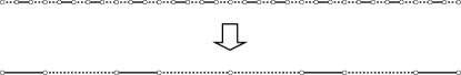
Figure 1: Left end of the Fibonacci XXZ chain with $J_{a}<J_{b}$. Dashed (solid) lines represent weak (strong) bonds, while circles indicate the positions of the spins. Apart from a few bonds close to the chain ends, the effective couplings also form a Fibonacci sequence.

First we apply the method to chains with Fibonacci couplings. This is the simplest example of the quasiperiodic precious-mean sequences with marginal fluctuations.Hermisson (2000) A few bonds closer to the left end of the original chain, along with induced effective couplings, are shown in Fig. 1 for $J_{a}<J_{b}$. In this case, only singlets are formed by the RG process; apart from a few bonds close to the chain ends, the renormalized lattice is again a Fibonacci chain. An effective coupling $J_{b}^{\prime}$ is induced between spins separated by only one singlet pair, while $J_{a}^{\prime}$ connects spins separated by two singlet pairs, and in terms of the original couplings we have

$$J_{a}^{\prime}=\gamma_{2}^{2}\frac{J_{a}^{3}}{J_{b}^{2}}\quad\text{and}\quad J_{b}^{\prime}=\gamma_{2}\frac{J_{a}^{2}}{J_{b}}.$$

The bare coupling ratio is $\rho=J_{a}/J_{b}$, its renormalized value being $\rho^{\prime}=\gamma_{2}\rho$. In each generation $j$, all decimated blocks have the same size $r_{j}$ and gap $\Lambda_{j}$ (proportional to the effective $J_{b}$ bonds). The recursion relations for $\rho$ and $\Lambda$ are given by

$$\rho_{j+1}=\gamma_{2}\rho_{j}\quad\text{and}\quad\Lambda_{j+1}=\gamma_{2}\rho_{j}^{2}\Lambda_{j}.$$ (10)

For the XX chain $\gamma_{2}=1$, and thus $\rho_{j+1}=\rho_{j}$, corresponding to a line of fixed points. On the other hand, for the Heisenberg chain $\gamma_{2}=\nicefrac{{1}}{{2}}$, so that $\rho_{j+1}<\rho_{j}$, leading to a stable fixed point $\rho_{\infty}=0$; since the perturbative approach on which the MDH scheme is based works for $\rho\ll 1$, the method can be expected to yield asymptotically exact results for the Heisenberg Fibonacci chains. In both cases, solving Eqs. (10) gives the gap in the $j$th generation in terms of the original coupling ratio $\rho$ and gap $\Lambda$,

$$\Lambda_{j}=\gamma_{2}^{j^{2}}\rho^{2j}\Lambda.$$

(Notice that, since $\gamma_{2}$ depends on the anisotropy, this last equation is valid only for $\Delta_{i}\equiv 0$ or $\Delta_{i}\equiv 1$; in the intermediate anisotropy regime, the variation of $\gamma_{2}$ along the generations must be taken into account.Hida (2004b)) The distance between spins forming a singlet in the $j$th generation defines a characteristic length $r_{j}$, corresponding to the Fibonacci numbers $r_{j}=1$, $3$, $13$, $55$, $\ldots$; for $j\gg 1$ the ratio $r_{j+1}/r_{j}$ approaches $\phi^{3}$, where $\phi=(1+\sqrt{5})/2$ is the golden mean. So we have $r_{j}\sim r_{0}\phi^{3j}$, where $r_{0}$ is a constant, and we obtain the dynamical scaling relation

$$\Lambda_{j}\sim r_{j}^{-\zeta}e^{-\mu\ln^{2}(r_{j}/r_{0})},$$ (11)

with $\zeta=-\nicefrac{{2}}{{3}}\ln\rho/\ln\phi$ and $\mu=-\ln\gamma_{2}/9\ln^{2}\phi$. For the Heisenberg chain ($\gamma_{2}=\nicefrac{{1}}{{2}}$), Eq. (11) describes a weakly exponential scaling (with a formally infinite dynamical exponent), but not of the form $\Lambda\sim\exp\left(-r^{\omega}\right)$ found for the XX chain with relevant aperiodicity ($\omega>0$). For the XX chain ($\gamma_{2}=1$), $\mu=0$ and we can identify $\zeta$ with a dynamical exponent $z$, whose value depends on the coupling ratio, leading to nonuniversal scaling behavior, characteristic of strictly marginal operators. (We can check that $z=\zeta$ corresponds to the asymptotic form of the exact XX expressionLuck and Nieuwenhuizen (1986); Hermisson (2000) for $\rho\ll 1$.) This nonuniversality should hold in the anisotropy regime $0<\Delta<1$ with a ‘bare’ value of $\rho$ defined at a crossover scale. Note that, taking into account the scaling form $\Lambda\sim\exp\left(-r^{\omega}\right)$ valid for relevant aperiodicity, we can view the above Heisenberg scaling form ($\mu\neq 0$) as a marginally relevant $(\omega\rightarrow 0^{+}$) case. The result in Eq. (11) has also been obtained in Ref. Hida, 2004a.

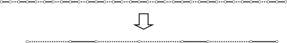
Figure 2: Left end of the Fibonacci chains with $J_{a}>J_{b}$. Effective spins form in the first lattice sweep, giving rise to a Fibonacci chain with the roles of the weak and strong bonds interchanged, exactly as in the original lattice in Fig. 1.

If we choose $J_{a}>J_{b}$, blocks with three spins connected by two strong bonds appear in the chain, producing effective spins upon renormalization. However, as illustrated in Fig. 2, the first lattice sweep yields again a Fibonacci chain with the roles of weak and strong bonds interchanged, exactly as in Fig. 1. The effective couplings in the second generation are given by

$$J_{a}^{\prime}=\gamma_{2}\gamma_{3}^{2}\frac{J_{b}^{2}}{J_{a}}\quad\textrm{and}\quad J_{b}^{\prime}=\gamma_{3}^{2}J_{b},$$ (12)

and the coupling ratio is now

$$\rho^{\prime}=\frac{J_{b}^{\prime}}{J_{a}^{\prime}}=\frac{1}{\gamma_{2}}\frac{J_{a}}{J_{b}}=\left(\gamma_{2}\rho\right)^{-1},$$

which is larger than one, showing that $J_{a}^{\prime}<J_{b}^{\prime}$. Thus, we can apply the same analysis as in the case with $J_{a}<J_{b}$, but now with ‘bare’ couplings given by Eq. (12). So, in the XX chain, since $\gamma_{2}=1$, the MDH method predicts scaling forms which are symmetric under $\rho\rightarrow 1/\rho$, in agreement with the exact treatment.Luck and Nieuwenhuizen (1986); Hermisson (2000)

The susceptibility $\chi(T)$ can be estimatedFisher (1994) by assuming that, at energy scale $\Lambda_{j}\sim T$, singlet pairs are effectively frozen, while unrenormalized spins are essentially free, contributing Curie terms to the susceptibility. Thus, if $n_{j}\sim r_{j}^{-1}$ is the number of surviving spins in the $j$th generation, $\chi(T\sim\Lambda_{j})\sim n_{j+1}/\Lambda_{j}.$ This already gives reasonable results, as indicated by comparison with those obtained for the XX chain from numerical diagonalization of finite chains,Vieira based on the free-fermion method.Lieb et al. (1961) However, a more useful approximation can be obtained by noting that, in the $j$th generation, we can view the resulting lattice as composed of ‘independent’ singlets in which a pair of spins is coupled via an XXZ interaction with effective bond and anisotropy parameters $J_{b}^{(j)}$ and $\Delta_{b}^{(j)}$. Since the fraction of such singlets with respect to the number of original bonds is $(n_{j}-n_{j+1})/2$, the free energy per site of the whole system, in the presence of an external field $h\rightarrow 0$, can be estimated as

$$f(h,T)=\frac{1}{2}\sum_{j}\frac{n_{j}-n_{j+1}}{2}F_{\mathrm{{pair}}}\left(J_{b}^{(j)},\Delta_{b}^{(j)};h,T\right),$$ (13)

where $F_{\mathrm{{pair}}}(J,\Delta;h,T)$ is the free energy of a pair of spins interacting via the Hamiltonian

$$H_{\mathrm{{pair}}}=J\left(S_{1}^{x}S_{2}^{x}+S_{1}^{y}S_{2}^{y}+\Delta S_{1}^{z}S_{2}^{z}\right)-h(S_{1}^{z}+S_{2}^{z}).$$

Iterating the recursion relations for the effective couplings $J_{a,b}$ and $\Delta_{a,b}$, we can determine their values in each generation, and evaluate numerically the sum in Eq. (13) to obtain the free energy. Thermodynamic properties such as the zero-field susceptibility $\chi$ and the specific heat $c$ can be obtained by the relations

$$\chi=-\left.\frac{\partial^{2}f}{\partial h^{2}}\right|_{h=0}\textrm{\quad and}\quad c=-T\frac{\partial^{2}f}{\partial T^{2}}.$$

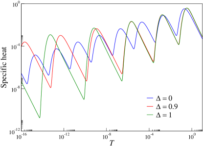
Figure 3: (Color online) Specific heat of the Fibonacci XXZ chains for $J_{a}/J_{b}=\nicefrac{{1}}{{10}}$ and three different values of the uniform anisotropy $\Delta$, as given by the ‘independent-singlet’ approximation.

As an example, Fig. 3 shows plots of the specific heat of Fibonacci XXZ chains with $J_{a}/J_{b}=\nicefrac{{1}}{{10}}$ and three values of the anisotropy $\Delta=\Delta_{a}=\Delta_{b}$, corresponding to the XX and Heisenberg limits and to an intermediate case ($\Delta=\nicefrac{{9}}{{10}}$). The results for the XX limit agree very well with those obtained from numerical diagonalization, although the agreement becomes worse for larger coupling ratios; in particular, the specific-heat scaling lawLuck and Nieuwenhuizen (1986); Hermisson (2000)

$$c(T)\sim T^{1/z}G_{c}\left(\frac{\ln T}{\ln\rho^{2}}\right),$$

with $z=\zeta(\rho)$ and $G_{c}$ a function of unit period, is fully satisfied, reflecting the strictly marginal character of the aperiodic perturbations. This is not the case in the Heisenberg limit, and the logarithmic amplitudes of the oscillations in the specific heat become larger with decreasing temperatures, reflecting the weakly exponential dynamical scaling in Eq. (11). For intermediate anisotropies, there is a crossover from Heisenberg-like to XX-like behavior as the temperature is lowered; the larger amplitude of the low-temperature oscillations corresponds to those of an XX chain with a ‘bare’ coupling ratio $\rho_{\mathrm{{eff}}}<\rho$ defined at a crossover scale in which effective anisotropies become negligible. (For a detailed analysis, see Ref. Hida, 2004b.)

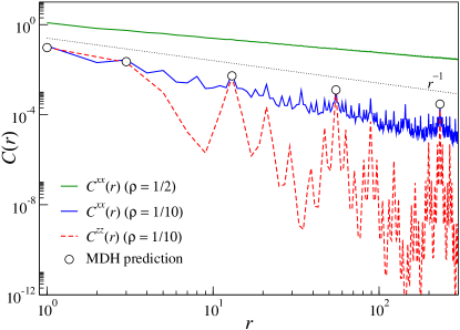
Figure 4: (Color online) Ground-state correlations as a function of the distance between spins for the Fibonacci XX chain. The curves are obtained from numerical diagonalization of closed chains with $2584$ sites. For $J_{a}/J_{b}=\nicefrac{{1}}{{10}}$ (lower curves), dominant correlations correspond to distances $r_{j}=1$, $3$, $13$, $55$ and $233$, for which $C^{xx}$ and $C^{zz}$ are nearly equal, as predicted by the MDH method (circles), and decay as $1/r$ (dotted curve). Larger coupling ratios lead to a slower decay of $C^{xx}$ (and a faster decay of $C^{zz}$), as seen for $J_{a}/J_{b}=\nicefrac{{1}}{{2}}$ (upper curve, offset for clarity).

As all singlets formed in the $j$th generation have length $r_{j}$ and the bond distribution is fixed, the average ground-state correlation between spins separated by a distance $r_{j}$ can be estimated as

$$C^{\alpha\alpha}(r_{j})\equiv\overline{\left\langle S_{i}^{\alpha}S_{i+r_{j}}^{\alpha}\right\rangle}\simeq\tfrac{1}{2}\left|c_{0}\right|\left(n_{j}-n_{j+1}\right)=\sigma\left|c_{0}\right|r_{j}^{-1},$$ (14)

where the bar denotes average over all possible pairs, $\sigma$ is a constant, $\alpha=x,y,z$, and $c_{0}$ is the correlation between the two spins in a singlet, given by $c_{0}=-\nicefrac{{1}}{{4}}$ for the Heisenberg chain and for both $\alpha=x$ and $\alpha=z$ in the XX chain. We point out that these should be the dominant correlations, and spins separated by distances other than $r_{j}$ are predicted to be only weakly correlated. As shown in Fig. 4, results from numerical diagonalization for the XX Fibonacci chain with $\rho=\nicefrac{{1}}{{10}}$ agree very well with the MDH predictions. Note that correlations in the uniform XX chain Lieb et al. (1961) decay as $C^{xx}(r)\sim r^{-1/2}$ and $C^{zz}(r)\sim r^{-2}$, so that dominant $xx$ ($zz$) correlations in the Fibonacci chain are weaker (stronger) than in the uniform chain. Due to the strictly marginal character of the fluctuations induced by the aperiodic couplings, deviations from the predictions in Eq. (14) appear in the XX chain for larger values of $\rho$, as also shown in the figure. This point will be further discussed in the next subsection, but these deviations should not be present in the Fibonacci Heisenberg chain, where aperiodicity can be viewed as marginally relevant.

V.2 The silver-mean sequence

Figure 5: Left end of the silver-mean chain with $J_{a}<J_{b}$. Effective couplings $J_{b}^{\prime}$ correspond to the original $J_{a}$ bonds, while $J_{a}^{\prime}$ connects spins separated by one singlet pair. Apart from the leftmost bond, the effective couplings also form a silver-mean sequence.

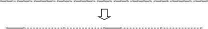
Figure 6: Left end of the silver-mean chain with $J_{a}>J_{b}$. Effective spins form in the first lattice sweep, producing the same structure as the third generation for $J_{a}<J_{b}$.

The silver-mean sequence is obtained from the substitution rule $a\rightarrow aab$, $b\rightarrow a$, and the rescaling factor predicted in the XX limit is Hermisson (2000)

$$\tau_{\mathrm{{sm}}}=1+\sqrt{2}.$$

When the MDH scheme is applied, the first lattice sweep also generates a silver-mean sequence, identical to the original one for $J_{a}<J_{b}$, but with the roles of weak and strong bonds interchanged for $J_{a}>J_{b}$, as shown in Figs. 5 and 6. In the latter case, the second-generation structure is identical to the third-generation lattice obtained for $J_{a}<J_{b}$, a situation we can assume without loss of generality. So, we can write the recursion relations

$$J_{a}^{\prime}=\gamma_{2}\frac{J_{a}^{2}}{J_{b}}\quad\textrm{and}\quad J_{b}^{\prime}=J_{a},$$

from which we get

$$\rho^{\prime}\equiv\frac{J_{a}^{\prime}}{J_{b}^{\prime}}=\gamma_{2}\frac{J_{a}}{J_{b}}\equiv\gamma_{2}\rho\quad\textrm{and}\quad\frac{\Lambda^{\prime}}{\Lambda}=\frac{J_{b}^{\prime}}{J_{b}}=\rho.$$

These are similar to the relations found for the Fibonacci chains. The length of singlets formed in the $j$th generation is $r_{j}=1,$ $1$, $3$, $7$, $17$, $41$, $\ldots$, whose asymptotic ratio is $r_{j+1}/r_{j}=\tau_{\mathrm{{sm}}}.$ Thus, solving the recursion relations yields

$$\Lambda_{j}\sim r_{j}^{-\zeta(\rho)}e^{-\mu\ln^{2}\left(r_{j}/r_{0}\right)},$$

with

$$\zeta(\rho)=-\frac{\ln\left(\gamma_{2}^{-\nicefrac{{1}}{{2}}}\rho\right)}{\ln\tau_{\mathrm{{sm}}}}\quad\textrm{and}\quad\mu=-\frac{\ln\left(\gamma_{2}^{\nicefrac{{1}}{{2}}}\right)}{\ln^{2}\tau_{\mathrm{{sm}}}},$$ (15)

so that in the XX limit the scaling again corresponds to a nonuniversal power-law behavior with a dynamical exponent $z=\zeta(\rho).$

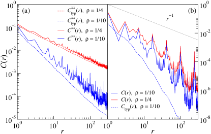
Figure 7: (Color online) Ground-state pair correlations in the silver-mean XX (a) and Heisenberg (b) chains, for $\rho=\nicefrac{{1}}{{4}}$ (upper curves) and $\rho=\nicefrac{{1}}{{10}}$ (lower curves), obtained from the second-order MDH scheme (chains with $8119$ sites). Solid and dashed curves correspond to average and typical correlations, respectively.

As in the Fibonacci chains, pair correlations in the ground state can be estimated by noting that only singlets are produced by the RG process, and we conclude that for $\rho\ll 1$ the dominant correlations (those between spins separated by the characteristic distances $r_{j}=1$, $3$, $7$, $17$,$\ldots$) should behave as

$$C(r_{j})\sim\frac{1}{r_{j}},$$

while correlations between spins separated by other distances should be negligible.

However, for XX chains, this is a rough approximation if the coupling ratio is not too small, and free-fermion calculations reveal a power-law decay of both $C^{xx}(r_{j})$ and $C^{zz}(r_{j})$ with $\rho$-dependent exponents, as in Fig. 4. This can be accounted for by the MDH method if we expand the ground-state vector to second-order in $\rho$, as described in Appendix B. Results of such calculations are shown in Fig. 7 for $\rho=\nicefrac{{1}}{{4}}$ and $\rho=\nicefrac{{1}}{{10}}$, in the XX and Heisenberg limits. Both average and typical correlations are plotted; the latter, defined by

$$C_{\mathrm{typ}}^{\alpha\alpha}(r)=\exp\left(\overline{\ln\left|\left\langle S_{i}^{\alpha}S_{i+r}^{\alpha}\right\rangle\right|}\right),$$

filter out the contribution of those pairs of spins most strongly correlated, yielding an estimate of the correlation between two arbitrary spins separated by a distance $r$. In the random-singlet phase, characteristic of random-bond chains,Fisher (1994) average correlations decay algebraically as $C(r)\sim 1/r^{2}$, whereas typical correlations are short-ranged, following $C_{\mathrm{typ}}(r)\sim\exp(-\sqrt{r/r_{0}})$. This is due to the fact that average correlations are dominated by the rare singlet pairs, while the correlation between a typical pair of spins is of the order of some intermediate effective coupling (see Appendix B).

As shown in Fig. 7(a), this picture does not hold for silver-mean XX spin chains. As the coupling ratio is lowered, average and typical correlations exhibit clearly distinct behavior, but both $C^{xx}(r_{j})$ and $C_{\mathrm{typ}}^{xx}(r)$ still follow approximately a power law, with $\rho$-dependent exponents, reproducing the results of the free-fermion calculations. This nonuniversality is related to the marginal character of the precious-mean fluctuations, which keeps the effective coupling ratio unchanged along the RG process, and can be qualitatively understood from the following argument. For each singlet pair coupled by a strong bond and whose spins are separated by a characteristic distance $r_{j}$, there exists a certain number of other spin pairs separated by the same distance $r_{j}$, but connected through weaker bonds, whose correlation (see Appendix B) is smaller than the strongest ones by factors of order $\rho$, $\rho^{2}$, $\rho^{3}$, etc. The average correlation can be estimated as

$$C^{xx}(r_{j})\sim\left(1+a_{1}\rho+a_{2}\rho^{2}+\cdots+a_{j}\rho^{j}\right)r_{j}^{-1},$$ (16)

where the $a_{n}$’s are proportional to the fractions of pairs giving contributions of order $\rho^{n}$, and the sum has an upper cutoff at $n=j$, since $r_{j}$ corresponds to the $j$th generation singlets. Assuming that $a_{n}=a_{1}\alpha^{n-1}$, for some constant $\alpha$ (which can be numerically checked to be a reasonable approximation for small $\rho$), we have

$$1+a_{1}\rho+a_{2}\rho^{2}+\cdots+a_{j}\rho^{j}=1+\frac{1-(\alpha\rho)^{j}}{1-\alpha\rho}a_{1}\rho,$$

and taking into account that $r_{j}\sim r_{0}\tau_{\mathrm{sm}}^{j}$ we can write

$$(\alpha\rho)^{j}\sim r_{j}^{1-\eta(\rho)},\quad\textrm{with}\quad\eta(\rho)=1-\frac{\ln(\alpha\rho)}{\ln\tau_{\mathrm{sm}}}.$$

Combining the above results we conclude that

$$C^{xx}(r_{j})\sim\frac{1}{r_{j}},$$

for $\rho<\alpha^{-1}$, reproducing the zeroth order MDH prediction, but a nonuniversal behavior

$$C^{xx}(r_{j})\sim\frac{1}{r_{j}^{\eta(\rho)}}$$

is obtained for $\rho>\alpha^{-1}$.

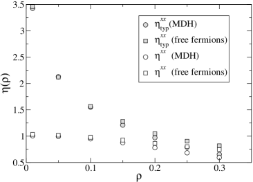
Figure 8: Decay exponents of $C^{xx}(r_{j})$ and $C_{\mathrm{typ}}^{xx}(r)$ for the XX silver-mean chain as a function of the coupling ratio $\rho=J_{a}/J_{b}$, obtained from both the second-order MDH scheme (chains with 8819 sites) and the free-fermion method (chains with 3363 sites). Errors bars are at most the same size as the symbols themselves.

For the silver-mean XX chains, an estimate of the $a_{n}$ based on numerical implementations of the MDH method gives $a_{1}\simeq 9.5$ and $\alpha\simeq 3$, but with some dependence on $r_{j}$ and $\rho$. As shown in Fig. 8, the decay exponent $\eta^{xx}$ of the average correlations approaches unity as $\rho\rightarrow 0$, but starts to decrease more rapidly for $\rho\gtrsim 0.1$, considerably less than $1/\alpha$; this discrepancy indicates that Eq. (16), with the assumption of constant $a_{n}$’s, although providing a valuable insight into the origin of the nonuniversal behavior, is not a good approximation for larger coupling ratios. The exponents predicted by the second-order MDH scheme are systematically smaller than the presumably exact ones obtained from the free-fermion method (which should tend to $\eta^{xx}=\nicefrac{{1}}{{2}}$ as $\rho\rightarrow 1$). This also happens for the decay exponent $\eta_{\mathrm{typ}}^{xx}$ of the typical correlations, which diverges as $\rho\rightarrow 0$, in agreement with the fact that, in this limit, the chain decomposes into independent singlets. A similar behavior is observed for the transverse correlations $C^{zz}(r)$ and $C_{\mathrm{{typ}}}^{zz}(r)$ (but now the decay exponents approach $\eta^{zz}=\eta_{\mathrm{{typ}}}^{zz}=2$ as $\rho\rightarrow 1$).

On the other hand, dominant ground-state correlations in the Heisenberg silver-mean chain closely follow the predictions of the zeroth-order MDH scheme, as can be seen in Fig. 7(b). This is due to the fact that the effective coupling ratio decreases as the RG proceeds, and the contribution to $C(r_{j})$ due to spin pairs other than those connected by strong bonds becomes exponentially negligible. Typical correlations decay not as a power law, but rather according to

$$C_{\mathrm{typ}}(r)\sim e^{-\mu_{\mathrm{{typ}}}\ln^{2}(r/r_{0})},$$

precisely the same form of the dynamical scaling; by fitting the numerical results, the constant $\mu_{\mathrm{{typ}}}$ is found to be approximately $\mu/2$, with $\mu$ given by Eq. (15). As in the random-singlet phase, the scaling form of the typical correlations is similar to that of the lowest gaps, reflecting the fact that two spins separated by a distance $r$ are basically uncorrelated until the energy scale is of order $\Lambda(r)$, when they become weakly correlated through an intervening spin taking part in a singlet pair.

V.3 The bronze-mean sequence

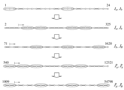
Figure 9: First five generations of the bronze-mean XXZ chain with $J_{a}<J_{b}$, each showing the leftmost $24$ sites. The numbers indicate the positions of the sites in the original chain. Encircled blocks contribute effective spins when renormalized. The labels on the right denote the effective bonds in each generation. The attractor of the block distribution is a two-cycle, reached at the second generation. All bonds to the right of the horizontal arrow follow the same sequence in the second (third) and fourth (fifth) generations.

The bronze-mean sequence is built from the substitution rule $a\rightarrow aaab$, $b\rightarrow a$, with a large XX rescaling factor Hermisson (2000)

$$\tau_{\mathrm{{bm}}}=\left(\frac{3+\sqrt{13}}{2}\right)^{3}\simeq 36.03.$$

The bond-distribution attractor produced by the MDH RG scheme is not a fixed point, but a two-cycle; apart from a few bonds near the chain ends, the same distributions alternate between even and odd generations, as shown for $J_{a}<J_{b}$ in Fig. 9. In this case, the second-generation couplings relate to the original couplings by

$$\tilde{J}_{a}=\gamma_{2}^{7}\gamma_{3}^{2}\frac{J_{a}^{5}}{J_{b}^{4}}\quad\textrm{and\quad}\tilde{J}_{b}=\gamma_{2}^{5}\gamma_{3}^{2}\frac{J_{a}^{4}}{J_{b}^{3}}.$$

Likewise, in terms of the couplings in the previous generation, we write the third-generation couplings,

$$\tilde{J}_{A}=\gamma_{3}^{2}\gamma_{4}\frac{\tilde{J}_{a}^{2}}{\tilde{J}_{b}}\quad\textrm{and\quad}\tilde{J}_{B}=\gamma_{3}^{2}\tilde{J}_{a},$$

and the fourth-generation couplings,

$$\tilde{J}_{a}^{\prime}=\gamma_{2}^{3}\gamma_{3}^{2}\frac{\tilde{J}_{A}^{4}}{\tilde{J}_{B}^{3}}\quad\textrm{and\quad}\tilde{J}_{b}^{\prime}=\gamma_{2}^{2}\gamma_{3}^{2}\frac{\tilde{J}_{A}^{3}}{\tilde{J}_{B}^{2}}.$$

Since the attractor is now a two-cycle, and not a fixed point, we must relate the couplings in the fourth and second-generations. By eliminating $\tilde{J}_{A}$ and $\tilde{J}_{B}$ in the above equations, we get

$$\tilde{J}_{a}^{\prime}=\gamma_{2}^{3}\gamma_{3}^{4}\gamma_{4}^{4}\frac{\tilde{J}_{a}^{5}}{\tilde{J}_{b}^{4}}\quad\textrm{and\quad}\tilde{J}_{b}^{\prime}=\gamma_{2}^{2}\gamma_{3}^{4}\gamma_{4}^{3}\frac{\tilde{J}_{a}^{4}}{\tilde{J}_{b}^{3}},$$

so that the coupling ratios satisfy the recursion relation

$$\tilde{\rho}^{\prime}\equiv\frac{\tilde{J}_{a}^{\prime}}{\tilde{J}_{b}^{\prime}}=\gamma_{2}\gamma_{4}\frac{\tilde{J}_{a}}{\tilde{J}_{b}}\equiv\gamma_{2}\gamma_{4}\tilde{\rho},$$

while the corresponding gaps are related by

$$\frac{\Lambda^{\prime}}{\Lambda}=\frac{\tilde{J}_{b}^{\prime}}{\tilde{J}_{b}}=\gamma_{2}^{2}\gamma_{3}^{4}\gamma_{2}^{3}\tilde{\rho}^{4}.$$

The distance between spins connected by strong bonds in the $j$th generation is $r_{j}=1$, $13$, $43$, $469$, $1549$,$\ldots$, which asymptotically gives $r_{j+2}/r_{j}=\tau_{\mathrm{{bm}}}$, so that $r_{2j}\sim r_{0}\tau_{\mathrm{{bm}}}^{j}$ . Thus, solving the recursion relations for $\tilde{\rho}$ and $\Lambda$, and taking into account that $\tilde{\rho}=\gamma_{2}^{2}\rho$, we obtain the dynamic scaling form

$$\Lambda_{2j}=r_{2j}^{-\zeta(\rho)}\exp\left(-\mu\ln^{2}\frac{r_{2j}}{r_{0}}\right),$$ (17)

with

$$\zeta(\rho)=-\frac{\ln\left(\gamma_{2}^{8}\gamma_{3}^{4}\gamma_{4}\rho^{4}\right)}{\ln\tau_{\mathrm{{bm}}}}\quad\textrm{and}\quad\mu=-\frac{\ln\left(\gamma_{2}^{2}\gamma_{4}\right)}{\ln^{2}\tau_{\mathrm{{bm}}}}.$$

Of course, the same form is obtained if we choose to look at the odd generations. In the XX limit, as $\gamma_{2}=\gamma_{4}=1$, we again have $\mu=0$ and Eq. (17) corresponds to a nonuniversal power-law scaling behavior, with a dynamical exponent $z=\zeta(\rho)$; once more, as in all marginal XX chains, $\zeta$ equals the leading term in the $\rho\ll 1$ expansion of the exact dynamical exponent.Hermisson (2000) As in the Fibonacci and silver-mean chains, choosing $J_{a}>J_{b}$ leads to the same scaling behavior, since after the first lattice sweep the bond distribution is essentially equal to the one obtained for $J_{a}<J_{b}$.

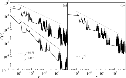
Figure 10: Ground-state correlation functions of the XX (a) and Heisenberg (b) bronze-mean chains, obtained from the zeroth-order MDH scheme (chains with $2\,010\,601$ sites).

Thus, the bronze-mean chains present qualitatively the same low-temperature thermodynamic behavior as the Fibonacci chain. However, this is not the case for ground-state properties. As indicated in Fig. 9, the renormalization process in each generation involves all spins in the chain, and gives rise to a hierarchy of effective spins, analogous to that shown in Fig. 11. As a consequence, an effective spin in the $j$th generation represents $3^{j-1}$ real spins. So, while the ground states of the Fibonacci and silver-mean chains could be described as ‘aperiodic singlet phases’, from which excitations of a given energy involve spins separated by a single, well-defined distance, low-energy excitations in the bronze-mean chain involve an exponentially large number of spin pairs, whose distances are distributed in an increasing range. This is reflected in the ground-state correlation functions, which exhibit a fractal-like structure, as seen in Fig. 10. The strongest correlations in the chains correspond to the distances $r_{2j}=13$, $469$, $16897$, $\ldots$, and their scaling behavior can be obtained by the following analysis.

Consider a pair of neighboring effective spins belonging to the same block in the $j$th generation, and let $c_{0}$ be their zeroth-order correlation. Each of these spins represents $3^{j-1}$ real spins, so that for each such pair there are $3^{j-1}$ pairs of real spins separated by the same distance $r_{j}$ contributing to the total correlation per site $C(r_{j})$. However, the contribution of a real pair to $C(r_{j})$ depends on the string of Clebsch-Gordan coefficients indicating the weight of its two spins in the effective spins: each time the intermediate effective spin representing a real spin $S_{k}$ is located at the ends (the center) of a three-spin block, the weight of $S_{k}$ is multiplied by a factor $c_{1,3}$ ($c_{2,3}$) upon renormalization. (These coefficients are in general different for $xx$ and $zz$ correlations; see Appendix A.) Since each effective spin in the $j$th generation has gone through $j-1$ renormalizations, a real pair can be classified according to the number $n$ of factors $c_{1,3}$ present in the (equal) weights of its spins. The contribution of all type-$n$ pairs to $C(r_{j})$ is proportional to the number of such pairs, being given by

$$g_{j}^{(n)}=2^{n}\frac{(j-1)!}{n!(j-1-n)!}\left(c_{1,3}^{2}\right)^{n}\left(c_{2,3}^{2}\right)^{j-1-n}\left|c_{0}\right|.$$

Thus, the total contribution of a single effective-spin pair to $C(r_{j})$ is

$$g_{j}=\sum_{n=0}^{j-1}g_{j}^{(n)}=\left(c_{2,3}^{2}+2c_{1,3}^{2}\right)^{j-1}\left|c_{0}\right|,$$

which gives

$$C(r_{j})\sim n_{j}g_{j}\sim\frac{\left(c_{2,3}^{2}+2c_{1,3}^{2}\right)^{j}}{r_{j}},$$

where $n_{j}$ is the fraction of active spins in the $j$th generation. Since asymptotically we have $j=\ln(r_{j}/r_{0})/\ln\sqrt{\tau_{\mathrm{bm}}}$, this last result can be written as

$$C(r_{j})\sim r_{j}^{-\eta},\quad\textrm{with}\quad\eta=1-\frac{\ln\left(c_{2,3}^{2}+2c_{1,3}^{2}\right)}{\ln\sqrt{\tau_{\mathrm{bm}}}}.$$ (18)

For the Heisenberg chain, $c_{1,3}=\gamma_{3}=\nicefrac{{2}}{{3}}$ and $c_{2,3}=\nicefrac{{1}}{{3}}$, so that $\eta=1$. For the XX chain, $\eta$ depends on whether we look at longitudinal or transverse correlations: in the former case we have $c_{1,3}^{xx}=\nicefrac{{1}}{{\sqrt{2}}}$ and $c_{2,3}^{xx}=\nicefrac{{1}}{{2}}$, so that $\eta^{xx}\simeq 0.875$, while in the latter case $c_{1,3}^{zz}=\nicefrac{{1}}{{2}}$, $c_{2,3}^{zz}=0$, and so $\eta^{zz}\simeq 1.387$. These values are fully compatible with the results from numerical implementations of the MDH scheme shown in Fig. 10, and agree very well with free-fermion calculations for XX chains with $\rho\ll 1$. Again, larger coupling ratios lead to nonuniversal decay of the correlations, except in the Heisenberg limit.

V.4 A sequence producing effective-spin triples

Figure 11: First three generations of the XXZ chain with couplings following the sequence in Sec. V.4, for $J_{a}<J_{b}$, showing an effective-spin hierarchy. Solid lines indicate strong bonds; for clarity, weak bonds are not represented. Shaded blocks contribute effective spins when renormalized, while white blocks form singlets. A third-generation effective spin represents three second-generation and nine first-generation spins.

The appearance of an effective-spin hierarchy is better illustrated by the sequence obtained from the substitution rule $a\rightarrow bbaba$, $b\rightarrow bba$. The first three generations of the chains, for $J_{a}<J_{b}$, are shown in Fig. 11; for $J_{a}>J_{b}$ the first lattice sweep interchanges the roles of weak and strong bonds, recovering the former case. Renormalization involves both three-spin and two-spin blocks, and each lattice sweep reproduces the original sequence, yielding effective couplings given by

$$J_{a}^{\prime}=\gamma_{2}\gamma_{3}^{2}\frac{J_{a}^{2}}{J_{b}}\quad\textrm{and}\quad J_{b}^{\prime}=\gamma_{3}^{2}J_{a},$$

so that the recursion relations for the coupling ratio and the energy gap are

$$\rho^{\prime}=\gamma_{2}\rho\quad\textrm{and}\quad\Lambda^{\prime}=\gamma_{3}^{2}\rho\Lambda.$$

The size of three-spin blocks follows $r_{j}=2$, $6$, $22$,$\ldots$, while that of two-spin blocks corresponds to $r_{j}/2$, leading asymptotically to a rescaling factor

$$\tau_{\mathrm{st}}=2+\sqrt{3}\simeq 3.73,$$

and a dynamical scaling relation

$$\Lambda_{j}\sim r_{j}^{-\zeta(\rho)}e^{-\mu\ln^{2}\left(r_{j}/r_{0}\right)},$$

with

$$\zeta(\rho)=-\frac{\ln\left(\gamma_{2}^{-\nicefrac{{1}}{{2}}}\gamma_{3}^{2}\rho\right)}{\ln\tau_{\mathrm{{st}}}}\quad\textrm{and}\quad\mu=-\frac{\ln\left(\gamma_{2}^{\nicefrac{{1}}{{2}}}\right)}{\ln^{2}\tau_{\mathrm{st}}}.$$

Again, aperiodicity induces nonuniversal behavior for $0\leq\Delta<1$, and a weakly exponential scaling in the Heisenberg limit.

As in the bronze-mean chains, discussed in the previous subsection, excitations of a given energy involve an exponentially large number of spins, due to the effective-spin hierarchy. More precisely, since each effective spin in $j$th generation represents $3^{j-1}$ real spins, excitations with energy $\Lambda_{j}$, corresponding to breaking a $j$th generation singlet, involve $2\cdot 3^{j-1}$ spins; exciting a three-spin block in the same generation costs an energy of the same order, and involves $3^{j}$ spins. Dominant ground-state correlation functions also decay as in Eq. (18), but now with

$$\eta=1-\frac{\ln\left(c_{2,3}^{2}+2c_{1,3}^{2}\right)}{\ln\tau_{\mathrm{st}}},$$

yielding $\eta^{xx}\simeq 0.830$ and $\eta^{zz}\simeq 1.526$ for the XX chain, and $\eta=1$ for the Heisenberg chain. These values are again fully compatible with results from numerical implementations of the MDH scheme.

V.5 A marginal tripling sequence

Figure 12: First two generations of the XXZ chain with couplings following the sequence in Sec. V.5, for $J_{a}<J_{b}$. The numbers indicate the position of the spins in the original chain. The first lattice sweep generates a fixed-point bond distribution with four different effective couplings $\tilde{J}_{a}$ through $\tilde{J}_{d}$.

This sequence is generated by the substitution rule $a\rightarrow aba$, $b\rightarrow bba$. As discussed in Ref. Hermisson, 2000, this type of aperiodicity may lead to marginal behavior even in anisotropic XY chains. As shown in Fig. 12, for $J_{a}<J_{b}$ the MDH scheme produces a second-generation lattice with four different effective couplings, given by

$$\tilde{J}_{a}=\gamma_{2}\gamma_{3}\frac{J_{a}^{2}}{J_{b}},\quad\tilde{J}_{b}=\gamma_{3}J_{a},$$

$$\tilde{J}_{c}=\gamma_{3}^{2}J_{a},\quad\tilde{J}_{d}=\gamma_{2}\frac{J_{a}^{2}}{J_{b}},$$

with an effective coupling ratio $\tilde{\rho}=\tilde{J}_{a}/\tilde{J}_{b}=\gamma_{2}\rho$. (Choosing $J_{a}>J_{b}$ interchanges the roles of $\tilde{J}_{c}$ and $\tilde{J}_{d}$, otherwise producing the same bond distribution.) The bond distribution does not change upon further lattice sweeps, and the effective couplings satisfy the recursion relations

$$\tilde{J}_{a}^{\prime}=\gamma_{2}\frac{\tilde{J}_{a}^{2}}{\tilde{J}_{b}},\quad\tilde{J}_{b}^{\prime}=\gamma_{2}\frac{\tilde{J}_{c}\tilde{J}_{d}}{\tilde{J}_{b}},$$

$$\tilde{J}_{c}^{\prime}=\gamma_{2}\frac{\tilde{J}_{a}\tilde{J}_{c}}{\tilde{J}_{b}},\quad\tilde{J}_{d}^{\prime}=\gamma_{2}\frac{\tilde{J}_{a}\tilde{J}_{d}}{\tilde{J}_{b}}.$$

Noting that $\tilde{J}_{a}=\tilde{J}_{c}\tilde{J}_{d}/\tilde{J}_{b},$ we can write

$$\tilde{\rho}^{\prime}=\frac{\tilde{J}_{a}^{\prime}}{\tilde{J}_{b}^{\prime}}=\frac{\tilde{J}_{a}}{\tilde{J}_{b}}=\tilde{\rho},$$

so that aperiodicity is marginal even in the Heisenberg limit. The recursion relation for the gaps is

$$\Lambda^{\prime}=\frac{\tilde{J}_{b}^{\prime}}{\tilde{J}_{b}}\Lambda=\gamma_{2}\tilde{\rho}\Lambda,$$

and the size of the singlets formed along the generations follows $r_{j}=3^{j}-1$, with a rescaling factor $\tau_{\mathrm{mt}}=3$, so that the dynamic scaling relation is given by

$$\Lambda_{j}\sim r_{j}^{-\zeta(\rho)},$$

with a nonuniversal dynamical exponent

$$z=\zeta(\rho)=-\frac{\ln\left(\gamma_{2}^{2}\rho\right)}{\ln 3}.$$

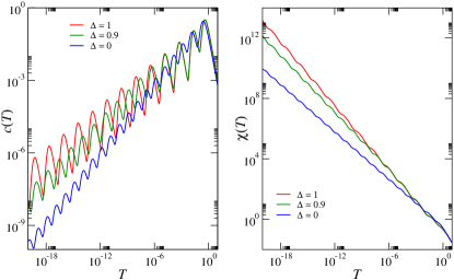
Figure 13: (Color online) Log-log plots of the specific heat $c(T)$ and susceptibility $\chi(T)$ as functions of temperature for XXZ chains with couplings following the marginal tripling sequence, for $J_{a}/J_{b}=\nicefrac{{1}}{{10}}$ and three different values of the uniform anisotropy $\Delta$.

Thermodynamic properties can be estimated by using the same idea of the ‘independent-singlet’ approximation described for Fibonacci chains, with slight modifications due to the fact that the first lattice sweep (but not the later ones) involves renormalization of both two- and three-spin blocks. Thus, the free energy per site can be calculated by adding to Eq. (13) a term representing the contribution of spins renormalized in the first lattice sweep, and given by

$$f_{1}(h,T)=\frac{1}{6}F_{\mathrm{pair}}(J_{b},\Delta_{b};h,T)+\frac{1}{6}F_{\mathrm{triple}}(J_{b},\Delta_{b};h,T),$$ (19)

where $F_{\mathrm{triple}}(J,\Delta;h,T)$ is the free energy of a spin triple obeying the Hamiltonian

$$\begin{array}[]{ccl}H_{\mathrm{triple}}&=&J\left(S_{1}^{x}S_{2}^{x}+S_{1}^{y}S_{2}^{y}+\Delta S_{1}^{z}S_{2}^{z}\right)\\ &+&J\left(S_{2}^{x}S_{3}^{x}+S_{2}^{y}S_{3}^{y}+\Delta S_{2}^{z}S_{3}^{z}\right)\\ &-&h(S_{1}^{z}+S_{2}^{z}+S_{3}^{z}).\end{array}$$

Notice that three-spin blocks yield effective spins when renormalized, and these will pair with other real or effective spins to form singlets in the second lattice sweep, but this is not taken into account by Eq. (19). In order to obtain a correct estimate of the low-temperature susceptibility, we must multiply the contribution arising from spin triples by a factor like $e^{-J_{b}/T}$. Results for the temperature dependence of the specific heat and susceptibility are shown in Fig. 13, for $\rho=\nicefrac{{1}}{{10}}$ and three values of the uniform anisotropy $\Delta$, corresponding to the XX and Heisenberg chains and to an intermediate case. Both quantities exhibit log-periodic oscillations, obeying the scaling forms

$$c(T)\sim T^{\nicefrac{{1}}{{z}}}G_{c}\left(\frac{\ln T}{\ln\lambda}\right)\quad\textrm{and}\quad\ \chi(T)\sim T^{\nicefrac{{1}}{{z}}-1}G_{\chi}\left(\frac{\ln T}{\ln\lambda}\right),$$

with $\lambda$ being the asymptotic ratio between the gaps in successive generations, while $G_{c}$ and $G_{\chi}$ are periodic functions (with period one). In the XX and Heisenberg limits, we have $\lambda=\gamma_{2}^{2}\rho$; for intermediate anisotropies, $\lambda$ equals $\rho_{\mathrm{eff}}$, a coupling ratio defined at the energy scale in which effective anisotropies become negligible.

Also as a consequence of the strictly marginal character of aperiodic fluctuations for all anisotropies in the regime $0\leq\Delta\leq 1$, dominant ground-state correlations follow $C(r_{j})\sim 1/r_{j}$ in the $\rho\ll 1$ regime, but nonuniversal behavior should be observed for larger coupling ratios.

VI Relevant aperiodicity

VI.1 The binary Rudin-Shapiro sequence

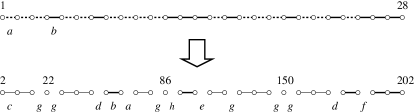
Figure 14: First two generations of the binary Rudin-Shapiro XXZ chain, for $J_{a}<J_{b}$. The first lattice sweep generates $8$ different effective couplings, $\tilde{J}_{a}$ through $\tilde{J}_{h}$, labeled in the figure by the letters $a-h$. Further renormalization does not change the bond distribution. Starting from the second generation, only blocks coupled by $\tilde{J}_{b}$ (thick lines) and $\tilde{J}_{c}$ (thin lines) bonds are renormalized. (For clarity, weaker bonds are not drawn in the picture.)

The Rudin-Shapiro sequence is originally defined as a four-letter sequence,Luck (1989) generated by the substitution rule $a\rightarrow ac$, $b\rightarrow dc$, $c\rightarrow ab$ and $d\rightarrow db$. It has the interesting property that its geometrical fluctuations mimic those induced by a random distribution. In order to reduce it to a binary sequence, we make the associations $c\equiv a$ and $d\equiv b$, obtaining an inflation rule for letter pairs, given by $aa\rightarrow aaab$, $ab\rightarrow aaba$, $ba\rightarrow bbab$ and $bb\rightarrow bbba$. The rule generates blocks having between $2$ and $5$ spins, and is symmetric under the interchange of $a$ and $b$, so that the scaling behavior is invariant with respect to the interchange of $J_{a}$ and $J_{b}$. The left-end of the first two generations of the Rudin-Shapiro chains is shown in Fig. 14 for $J_{a}<J_{b}$.

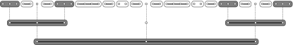
Figure 15: Pattern of three-spin blocks and isolated spins leading to the effective-spin hierarchy in Rudin-Shapiro XXZ chains. Thick lines indicate strong bonds. Shaded blocks contribute effective spins when renormalized; white blocks form singlets.

Blocks with more than $3$ spins are eliminated in the first lattice sweep and do not appear in later generations. Both two- and three-spin blocks are present in the fixed-point block distribution (already reached at the second generation), and upon renormalization the sequence produces an effective-spin hierarchy, stemming from approximately mirror-symmetric patterns of three-spin and five-spin blocks in the original lattice. This is illustrated in Figs. 15 and 16.

Figure 16: Pattern of five-spin and three-spin blocks leading to the effective-spin hierarchy in Rudin-Shapiro XXZ chains. Thick lines indicate strong bonds. Shaded blocks contribute effective spins when renormalized; white blocks form singlets.

In the $j$th generation, three-spin blocks have size $r_{j}=2\cdot 4^{j-1}$ (with a rescaling factor $\tau_{\mathrm{rs}}=4$), while two-spin blocks have size $r_{j}/2$. The first lattice sweep generates effective couplings $\tilde{J}_{i}$ having 8 different values,

$$\tilde{J}_{a}=\gamma_{2}\gamma_{3}\gamma_{4}\frac{J_{a}^{5}}{J_{b}^{4}},\quad\tilde{J}_{b}=\gamma_{3}\gamma_{5}J_{a},$$

$$\tilde{J}_{c}=\gamma_{2}\gamma_{3}\frac{J_{a}^{2}}{J_{b}},\quad\tilde{J}_{d}=\gamma_{3}\gamma_{4}\gamma_{5}\frac{J_{a}^{2}}{J_{b}},\quad\tilde{J}_{e}=\gamma_{2}^{2}\gamma_{3}\gamma_{5}\frac{J_{a}^{2}}{J_{b}},$$

$$\tilde{J}_{f}=\gamma_{2}^{2}\gamma_{3}\gamma_{4}\gamma_{5}\frac{J_{a}^{3}}{J_{b}^{2}},\quad\tilde{J}_{g}=\gamma_{2}^{2}\gamma_{3}\gamma_{4}\frac{J_{a}^{4}}{J_{b}^{3}},\quad\tilde{J}_{h}=\gamma_{2}^{3}\gamma_{3}\gamma_{4}^{2}\frac{J_{a}^{5}}{J_{b}^{4}},$$

and whose bond distribution remains unchanged upon renormalization, leading to the recursion relations

$$\tilde{J}_{a}^{\prime}=\gamma_{2}^{3}\frac{\tilde{J}_{a}^{2}\tilde{J}_{d}\tilde{J}_{g}}{\tilde{J}_{b}\tilde{J}_{c}^{2}},\quad\tilde{J}_{b}^{\prime}=\gamma_{3}\tilde{J}_{f},$$

$$\tilde{J}_{c}^{\prime}=\gamma_{3}\tilde{J}_{g},\quad\tilde{J}_{d}^{\prime}=\gamma_{2}\gamma_{3}^{2}\frac{\tilde{J}_{d}\tilde{J}_{f}}{\tilde{J}_{b}},\quad\tilde{J}_{e}^{\prime}=\gamma_{2}\gamma_{3}^{2}\frac{\tilde{J}_{e}\tilde{J}_{g}}{\tilde{J}_{c}},$$

$$\tilde{J}_{f}^{\prime}=\gamma_{2}^{2}\gamma_{3}\frac{\tilde{J}_{a}\tilde{J}_{d}\tilde{J}_{f}}{\tilde{J}_{b}\tilde{J}_{c}^{2}},\quad\tilde{J}_{g}^{\prime}=\gamma_{2}^{2}\gamma_{3}\frac{\tilde{J}_{a}\tilde{J}_{d}\tilde{J}_{g}}{\tilde{J}_{b}\tilde{J}_{c}},\quad\tilde{J}_{h}^{\prime}=\gamma_{2}^{3}\frac{\tilde{J}_{e}\tilde{J}_{f}\tilde{J}_{h}^{2}}{\tilde{J}_{b}^{2}\tilde{J}_{c}}.$$

Defining a new effective coupling $\tilde{J}_{0}=\tilde{J}_{a}\tilde{J}_{d}/\tilde{J}_{c}$, we obtain a system of three recursion relations,

$$\tilde{J}_{0}^{\prime}=\gamma_{2}^{4}\gamma_{3}\frac{\tilde{J}_{0}^{2}\tilde{J}_{f}}{\tilde{J}_{b}^{2}},\quad\tilde{J}_{b}^{\prime}=\gamma_{3}\tilde{J}_{f},\quad\textrm{and}\quad\tilde{J}_{f}^{\prime}=\gamma_{2}^{2}\gamma_{3}\frac{\tilde{J}_{0}\tilde{J}_{f}}{\tilde{J}_{b}}.$$

With coupling ratios $\tilde{\rho}=\tilde{J}_{0}/\tilde{J}_{b}$ and $\tilde{\sigma}=\tilde{J}_{f}/\tilde{J}_{b}$, and a gap proportional to $\tilde{J}_{b}$, we have

$$\tilde{\rho}_{j}=\gamma_{2}^{4}\tilde{\rho}_{j-1}^{2},\quad\tilde{\sigma}_{j}=\gamma_{2}^{2}\tilde{\rho}_{j-1},\quad\textrm{and }\quad\frac{\Lambda_{j}}{\Lambda_{j-1}}=\gamma_{3}\tilde{\sigma}_{j},$$

which after eliminating $\tilde{\sigma}_{j}$ yields

$$\tilde{\rho}_{j}=\gamma_{2}^{4}\tilde{\rho}_{j-1}^{2}\quad\textrm{and}\quad\frac{\Lambda_{j}}{\Lambda_{j-1}}=\gamma_{3}\tilde{\rho}_{j}^{\nicefrac{{1}}{{2}}}.$$

Solving the recursion relations we obtain

$$\Lambda_{j}\sim r_{j}^{-\zeta}\exp\left[-\mu\left(\frac{r}{r_{0}}\right)^{\omega}\right],$$

with $\omega=\nicefrac{{1}}{{2}}$,

$$\zeta=\frac{\ln\left(\gamma_{3}/\gamma_{2}^{2}\right)}{\ln\tau_{\mathrm{rs}}}\quad\textrm{and}\quad\mu=-\frac{1}{2}\ln\left(\gamma_{2}^{2}\gamma_{4}\rho^{2}\right).$$

So we obtain, for the whole regime $0\leq\Delta\leq 1$, the dynamical scaling form predicted for the XX chain, reproducing the result for the random-singlet phase.

Figure 17: Ground-state correlations for chains with Rudin-Shapiro couplings, obtained from extrapolation of numerical MDH results for chains with $2^{16}$ to $2^{20}$ sites. (a) $C^{xx}(r)$ (upper solid curve) and $C^{zz}(r)$ (lower solid curve) for the XX chain. The dotted curve is proportional to $r^{-3/2}$. (Curves offset for clarity.) Inset: dominant $C^{xx}$ correlations, corresponding to distances $r_{j}=2\cdot 4^{j-1}$, fitted by a law of the form $rC^{xx}(r)=y_{0}+y_{1}\ln r$ (dashed curve). (b) $C(r)$ for the Heisenberg chain (solid curve). The dotted curve is proportional to $1/r$.

For chains with RS couplings, effective-spin formation determines the dominant ground-state correlations, but the corresponding hierarchy is slightly different from the ones seen in Secs. V.3 and V.4, now involving both three-spin (and some five-spin) blocks and unrenormalized spins. As illustrated in Figs. 15 and 16, for each block renormalized in the $j$th generation the correlation between its end spins connects a number of order $2^{j}$ original spin pairs separated by the same distance $r_{j}$ (the size of the block), yielding a contribution to the average correlation in the Heisenberg chain and $C^{xx}(r_{j})$ in the XX chain given by

$$g_{j}=\left[\left(2c_{1,3}^{2}\right)^{j-1}+c_{2,3}^{2}\sum_{k=1}^{j-1}\left(2c_{1,3}^{2}\right)^{k-1}\right]\left|c_{0}\right|,$$

where $c_{0}$ is the correlation between end spins in a three-spin block. For the Heisenberg chain $2c_{1,3}^{2}=\nicefrac{{8}}{{9}}<1$, and thus

$$C(r_{j})\sim g_{j}n_{j}\sim\frac{1}{r_{j}},$$ (20)

where $n_{j}\sim 1/r_{j}$ is the fraction of three-spin blocks in the $j$th generation. For the XX chain $2\left(c_{1,3}^{xx}\right)^{2}=1$, so that $g_{j}$ has a term proportional to $j$, and $C^{xx}(r_{j})$ carries a logarithmic correction,

$$C^{xx}(r_{j})\sim g_{j}n_{j}\sim\left(y_{0}+y_{1}\ln r_{j}\right)r_{j}^{-1},$$ (21)

where $y_{0}$ and $y_{1}$ are constants. The $zz$ correlation between end spins in a three-spin block is zero, so that the dominant correlations correspond to spin pairs (connected through one of the effective end spins and the middle spin) at distances $r_{j}^{\prime}=4^{j-1}\pm 4^{j-2}\pm 4^{j-3}\pm\cdots\pm 1$, with average $\langle r_{j}^{\prime}\rangle=4^{j-1}$, whose contribution is given by $g_{j}^{\prime}\sim 1/2^{j-1}$, since $c_{1,3}^{zz}=\nicefrac{{1}}{{2}}$. We then have

$$C^{zz}(r_{j}^{\prime})\sim g_{j}^{\prime}n_{j}\sim\left\langle r_{j}^{\prime}\right\rangle^{-3/2}.$$ (22)

Eqs. (21) and (22) should be contrasted with the random-singlet isotropic result $C(r)\sim r^{-2}$, indicating a clear distinction between the ground-state phases induced by disorder and aperiodicity, even in the presence of similar geometric fluctuations. This is related to the inflation symmetry of the aperiodic sequences, which is absent in the random-bond case (or in aperiodic systems with random perturbations Arlego (2002)). Its effects are exemplified by the fractal structure of the ground-state correlations visible in Fig. 17, which displays results from numerical implementations of the MDH method for both XX and Heisenberg chains, showing conformance to the scaling forms in Eqs. (20)-(22). Contrary to the marginal sequences, these scaling forms should be observed in the large-distance behavior of Rudin-Shapiro XXZ chains for any coupling ratio $\rho\neq 1$; we expect a crossover from the uniform to aperiodic scaling behavior as larger distances are probed for $\rho$ close to unity. Free-fermion calculations in the XX limit support this picture.

VI.2 The 6-3 sequence

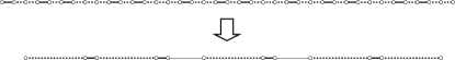
Figure 18: First two generations of the 6-3 sequence, discussed in Sec. VI.2, for $J_{a}<J_{b}$. In the second generation, dashed lines indicate effective $\tilde{J}_{a}$ bonds, while thick and thin solid lines denote effective $\tilde{J}_{b}$ and $\tilde{J}_{c}$ bonds. In subsequent generations, the $\tilde{J}_{c}\tilde{J}_{a}$ pairs change to $\tilde{J}_{a}\tilde{J}_{c}$, and the first $\tilde{J}_{a}$ becomes $\tilde{J}_{c}$, but the bond distribution is otherwise unchanged.

This sequence is generated by the substitution $a\rightarrow babaaa$, $b\rightarrow baa$, and its XX wandering exponent is $\omega=\ln 2/\ln 5$, with a rescaling factor $\tau_{63}=5$. Application of the MDH scheme leads to a fixed-point bond distribution with singlet renormalization only, so that no effective-spin hierarchy is present. For $J_{a}<J_{b}$, as depicted in Fig. 18, three effective couplings are produced after the first lattice sweep,

$$\tilde{J}_{a}=\gamma_{2}^{2}\frac{J_{a}^{3}}{J_{b}^{2}},\quad\tilde{J}_{b}=J_{a},\quad\tilde{J}_{c}=\gamma_{2}\frac{J_{a}^{2}}{J_{b}},$$

and upon further lattice sweeps we obtain the recursion relations

$$\tilde{J}_{a}^{\prime}=\gamma_{2}^{3}\frac{\tilde{J}_{a}^{3}\tilde{J}_{c}}{\tilde{J}_{b}^{3}},\quad\tilde{J}_{b}^{\prime}=\gamma_{2}\frac{\tilde{J}_{a}\tilde{J}_{c}}{\tilde{J}_{b}},\quad\tilde{J}_{c}^{\prime}=\gamma_{2}^{2}\frac{\tilde{J}_{a}^{2}\tilde{J}_{c}}{\tilde{J}_{b}^{2}}.$$

Thus, defining the effective coupling ratios

$$\tilde{\rho}\equiv\frac{\tilde{J_{a}}}{\tilde{J}_{b}}=\gamma_{2}^{2}\left(\frac{J_{a}}{J_{b}}\right)^{2}\quad\textrm{and}\quad\tilde{\sigma}=\frac{\tilde{J}_{c}}{\tilde{J}_{b}}=\gamma_{2}\frac{J_{a}}{J_{b}},$$

we can rewrite the recursion relations as

$$\tilde{\rho}^{\prime}=\gamma_{2}^{2}\tilde{\rho}^{2},\quad\tilde{\sigma}^{\prime}=\gamma_{2}\tilde{\rho},\quad\textrm{and}\quad\frac{\Lambda^{\prime}}{\Lambda}=\frac{\tilde{J}_{b}^{\prime}}{\tilde{J}_{b}}=\gamma_{2}\tilde{\sigma}\tilde{\rho}.$$

In the $j$th generation, we have $\tilde{\sigma}_{j}^{2}=\tilde{\rho}_{j}$, and thus

$$\tilde{\rho}_{j+1}=\gamma_{2}^{2}\tilde{\rho}_{j}^{2}\quad\textrm{and}\quad\Lambda_{j+1}=\gamma_{2}\tilde{\rho}_{j}^{\nicefrac{{3}}{{2}}}\Lambda_{j}.$$

The length of the singlets correspond to $r_{j}=1$, $9$, $45$, $225$,$\ldots$, so that asymptotically $r_{j}\sim r_{0}\tau^{j}$, with $r_{0}=\nicefrac{{9}}{{25}}$ and $\tau=\tau_{63}=5$. Solving the above recursion relations we obtain the dynamical scaling behavior,

$$\Lambda_{j}\sim r_{j}^{-\zeta}\exp\left[-\mu\left(\frac{r}{r_{0}}\right)^{\omega}\right],$$ (23)

with a wandering exponent $\omega=\ln 2/\ln 5\simeq 0.431$ and

$$\zeta=\frac{3\ln\gamma_{2}}{\ln 5}\quad\textrm{and}\quad\mu=-\frac{3}{2}\ln\left(\gamma_{2}^{4}\rho^{3}\right),$$

where $\rho=J_{a}/J_{b}$ is the original coupling ratio.

If we choose $J_{a}>J_{b}$, blocks with $2$, $3$ and $4$ spins coupled by strong bonds appear along the chain. Effective spins are produced by the first lattice sweep, yielding effective couplings

$$\tilde{J}_{a}=\gamma_{2}^{3}\gamma_{3}^{2}\gamma_{4}^{3}\frac{J_{b}^{7}}{J_{a}^{6}},\quad\tilde{J}_{b}=\gamma_{2}\gamma_{3}^{2}\gamma_{4}\frac{J_{b}^{3}}{J_{a}^{2}},\quad\textrm{and}\quad\tilde{J}_{c}=\gamma_{2}^{2}\gamma_{3}^{2}\gamma_{4}^{2}\frac{J_{b}^{5}}{J_{a}^{4}},$$

whose distribution is the same as that of the third-generation bonds for $J_{a}<J_{b}$, and which remains unchanged upon renormalization. Thus, the scaling behavior is the same as above, but now with a ‘bare’ coupling ratio

$$\tilde{\rho}\equiv\frac{\tilde{J}_{a}}{\tilde{J}_{b}}=\gamma_{2}^{2}\gamma_{4}^{2}\left(\frac{J_{b}}{J_{a}}\right)^{4}.$$

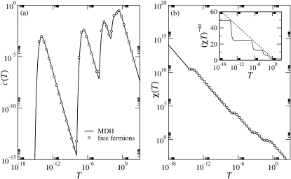
Figure 19: Thermal dependence of the specific heat (a) and susceptibility (b) of the XX chain with couplings following the 6-3 sequence of Sec. VI.2, obtained for $J_{a}/J_{b}=\nicefrac{{1}}{{4}}$ from both numerical diagonalization of chains with $46875$ sites (circles), and the MDH scheme (solid curves). The inset in (b) presents a log-linear plot of $T$ versus $(\chi T)^{-\omega}$, with $\omega=\ln 2/\ln 5$, showing that for $T\simeq\Lambda_{j}$, corresponding to the specific-heat maxima, the susceptibility satisfies the scaling form $\chi\sim T^{-1}\left|\ln T\right|^{-1/\omega}$ (dashed line); at intermediate temperatures, a Curie-like behavior is observed.

Thermodynamic properties can be estimated as in the Fibonacci case, by using the ‘independent-singlet’ approximation. Plots of the specific heat $c(T$) and susceptibility $\chi(T)$ as functions of temperature are shown in Fig. 19, and compare quite well with results from numerical diagonalization, even for relatively large coupling ratios ($J_{a}/J_{b}=\nicefrac{{1}}{{4}}$). This is not surprising, given the fact that the effective coupling ratio rapidly decreases as the RG proceeds, even for the XX chain. As seen in the inset of Fig. 19(b), at temperatures of the order of the gaps $\Lambda_{j}$ the susceptibility follows the scaling form

$$\chi(T)\sim\frac{1}{T\left|\ln T\right|^{1/\omega}},$$

which can be readily obtained from Eq. (23) by assuming that singlet pairs are magnetically frozen, while active spins contribute Curie terms to $\chi$. Estimates of $c(T)$ and $\chi(T)$ for chains with anisotropies $0<\Delta\leq 1$ are qualitatively identical to the ones for the XX chain.

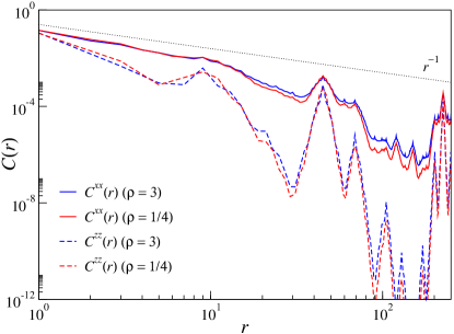
Figure 20: (Color online) Ground-state correlations of the XX chain with couplings following the 6-3 sequence of Sec. VI.2, for two different values of the coupling ratio $\rho=J_{a}/J_{b}$, as obtained by numerical diagonalization of chains with $1874$ sites. Peaks in the curves correspond to the characteristic distances $r_{j}=9$, $45$ and $225$.

Since no effective-spin hierarchy is present, and aperiodicity is relevant, dominant ground-state correlations, for any coupling ratio $\rho\neq 1$ and sufficiently large characteristic distances $r_{j}$, should decay as

$$C^{xx}(r_{j})\sim C^{zz}(r_{j})\sim\frac{1}{r_{j}},$$

for all anisotropies in the regime $0\leq\Delta\leq 1$. This is confirmed in the XX limit by numerical diagonalization, as shown in Fig. 20.

VI.3 The fivefold-symmetry sequence

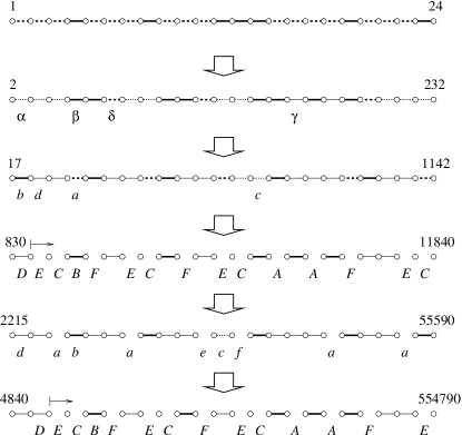
Figure 21: Leftmost 24 sites in the first six generations of XXZ chains with couplings following the fivefold-symmetry sequence, discussed in Sec. VI.3, for $J_{a}<J_{b}$. The attractor of the bond distribution is a two-cycle, reached after three lattice sweeps. Second-generation bonds are denoted by $J_{\alpha}$ through $J_{\delta}$; third- and fifth-generation couplings are labeled $a$ through $f$, while $A$ through $G$ label fourth- and sixth-generation bonds. Couplings $J_{G}$ only occur much farther along the chains. Starting from the fourth generation, lines indicate blocks to be renormalized.

The sequence produced by the substitution rule $a\rightarrow aaab$, $b\rightarrow bba$ is related to binary tilings of the plane with fivefold symmetry.Godrèche and Luck (1992) The (quite large) XX rescaling factor is $\tau_{\mathrm{ff}}=25+10\sqrt{5}\simeq 47.36$, with a wandering exponent $\omega=\ln 3/\ln\tau_{\mathrm{ff}}\simeq 0.285$.

Under a numerical implementation of the MDH scheme with $J_{a}<J_{b}$, we obtain a quite intricate pattern: after a four-bond transient produced by the first two lattice sweeps, a two-cycle periodic attractor is reached, where six- and seven-bond distributions alternate, as depicted in Fig. 21. (With $J_{a}>J_{b},$ the same two-cycle is reached after the first lattice sweep.) The distance between spins connected by the strongest bonds in each generation correspond to $r_{j}=1$, $3$, $33$, $190$, $1385$, $9050$, $\ldots$, which asymptotically gives $r_{j+2}/r_{j}\simeq\tau_{\mathrm{ff}}$ . The equations relating the effective couplings of the fourth and fifth generations are

$$\tilde{J}_{a}=\gamma_{2}^{3}\gamma_{3}\frac{\tilde{J}_{A}^{2}\tilde{J}_{C}\tilde{J}_{F}}{\tilde{J}_{B}^{3}},\quad\tilde{J}_{b}=\gamma_{3}\tilde{J}_{E},\quad\tilde{J}_{c}=\gamma_{2}^{2}\frac{\tilde{J}_{A}\tilde{J}_{C}\tilde{J}_{G}}{\tilde{J}_{B}^{2}},$$

$$\tilde{J}_{d}=\gamma_{2}^{2}\frac{\tilde{J}_{C}\tilde{J}_{E}\tilde{J}_{F}}{\tilde{J}_{B}\tilde{J}_{D}},\quad\tilde{J}_{e}=\gamma_{3}^{2}\frac{\tilde{J}_{A}^{2}\tilde{J}_{C}\tilde{J}_{G}}{\tilde{J}_{B}^{3}},\quad\tilde{J}_{f}=\gamma_{2}^{2}\gamma_{3}\frac{\tilde{J}_{A}\tilde{J}_{C}\tilde{J}_{F}}{\tilde{J}_{B}^{2}},$$

while between the couplings of the fifth and fourth generations we have

$$\tilde{J}_{A}^{\prime}=\gamma_{2}^{2}\gamma_{3}\frac{\tilde{J}_{e}^{2}\tilde{J}_{f}}{\tilde{J}_{b}\tilde{J}_{c}},\quad\tilde{J}_{B}^{\prime}=\gamma_{2}\gamma_{3}\frac{\tilde{J}_{d}\tilde{J}_{f}}{\tilde{J}_{b}},\quad\tilde{J}_{C}^{\prime}=\gamma_{2}\frac{\tilde{J}_{e}\tilde{J}_{f}}{\tilde{J}_{b}},$$

$$\tilde{J}_{D}^{\prime}=\gamma_{2}^{6}\gamma_{3}^{2}\frac{\tilde{J}_{a}^{2}\tilde{J}_{d}\tilde{J}_{e}\tilde{J}_{f}}{\tilde{J}_{b}^{3}\tilde{J}_{c}},\quad\tilde{J}_{E}^{\prime}=\gamma_{2}^{6}\gamma_{3}\frac{\tilde{J}_{a}^{2}\tilde{J}_{e}^{2}\tilde{J}_{f}}{\tilde{J}_{b}^{3}\tilde{J}_{c}},$$

$$\tilde{J}_{F}^{\prime}=\gamma_{2}^{8}\gamma_{3}^{2}\frac{\tilde{J}_{a}^{3}\tilde{J}_{d}\tilde{J}_{e}\tilde{J}_{f}}{\tilde{J}_{b}^{4}\tilde{J}_{c}},\quad\tilde{J}_{G}^{\prime}=\gamma_{2}^{8}\gamma_{3}\frac{\tilde{J}_{a}^{3}\tilde{J}_{e}^{2}\tilde{J}_{f}}{\tilde{J}_{b}^{4}\tilde{J}_{c}}.$$

Eliminating the fifth-generation couplings and defining the ratios

$$\tilde{\rho}=\frac{\tilde{J}_{A}}{\tilde{J}_{B}},\quad\sigma_{1}=\frac{\tilde{J}_{C}}{\tilde{J}_{B}},\quad\sigma_{2}=\frac{\tilde{J}_{F}^{2}}{\tilde{J}_{A}\tilde{J}_{B}},\textrm{\quad and}\quad\sigma_{3}=\frac{\tilde{J}_{F}}{\tilde{J}_{E}},$$

we can write a set of four recursion relations,

$$\tilde{\rho}^{\prime}=\gamma_{2}^{3}\tilde{\rho}_{j}^{3},\quad\sigma_{1}^{\prime}=\frac{\gamma_{2}}{\gamma_{3}}\tilde{\rho}^{2},$$

$$\sigma_{2}^{\prime}=\gamma_{2}^{22}\gamma_{3}\tilde{\rho}^{9}\left(\sigma_{1}\sigma_{3}\right)^{4},\quad\sigma_{3}^{\prime}=\gamma_{2}^{4}\gamma_{3}\sigma_{1}\sigma_{3}.$$

The gaps in successive even generations obey

$$\frac{\Lambda^{\prime}}{\Lambda}=\frac{\tilde{J}_{B}^{\prime}}{\tilde{J}_{B}}=\gamma_{2}^{5}\gamma_{3}\rho\sigma_{1}^{2}\sigma_{2},$$

and by expressing $\sigma_{1}$, $\sigma_{2}$ and $\sigma_{3}$ in terms of $\tilde{\rho}$ we get

$$\frac{\Lambda_{j+1}}{\Lambda_{j}}=a\gamma_{2}^{20j}\tilde{\rho}_{j}^{\nicefrac{{16}}{{3}}},$$

where now $2j+2$ labels the lattice generation and $a$ is a constant depending on the values of the coupling ratios in the fourth generation. Solving this last equation gives

$$\Lambda_{j}\sim A^{j}B^{j^{2}}C^{3^{j}},$$

with

$$A=a\gamma_{2}^{-8},\quad B=\gamma_{2}^{20},\quad\textrm{and}\quad C=\gamma_{2}^{4/9}\tilde{\rho}_{1}^{8/9}.$$

For large enough $j$, since $j=\ln(r_{j}/r_{0})/\ln\tau_{\mathrm{{ff}}}$, we have

$$\Lambda_{j}\sim\exp\left[-\mu\left(\frac{r_{j}}{r_{0}}\right)^{\omega}\right],$$

with

$$\mu=-\ln C\quad\textrm{and}\quad\omega=\frac{\ln 3}{\ln\tau_{\mathrm{{ff}}}},$$

again obtaining, for the whole anisotropy regime $0\leq\Delta\leq 1$, the same scaling form predicted for the XX chain.

The effective-spin hierarchy produced by the RG process is analogous to that in the bronze-mean chains, so that ground-state correlations behave as in Eq. (18), with $\eta=1$ in the Heisenberg chain, but $\eta^{xx}\simeq 0.884$ and $\eta^{zz}\simeq 1.359$ in the XX limit. However, these figures are not so well reproduced in the numerical calculations, even for chains with $N\simeq 1.6\times 10^{6}$ sites, most probably due to the extremely large rescaling factor.

VII Discussion and conclusions

For all aperiodic sequences discussed in the previous sections, the recursion relations for the main coupling ratio and the energy gaps have the forms

$$\rho_{j+1}=c\rho_{j}^{k}\quad\text{and}\quad\Lambda_{j+1}=f_{1}f_{2}^{j}\rho_{j}^{\ell}\Lambda_{j},$$ (24)

where $c$, $f_{1}$ and $f_{2}$ are $\Delta$-dependent nonuniversal constants, and $\ell$ (a rational number) and $k$ (an integer) relate to the number of singlets involved in determining the effective couplings. In particular, $k$ is ultimately the difference in the number of singlets producing the effective couplings whose ratio is $\rho<1$.

If $k\geq 2$, the recursion relation for $\rho$ always has a stable fixed point at $\rho^{*}=0$, so that the effective coupling ratios become exponentially small as the renormalization proceeds, indicating that asymptotic results obtained from the MDH method should be essentially exact. Taking into account the scaling behavior of the characteristic distances $r_{j}\sim r_{0}\tau^{j}$, Eqs. (24) lead to the dynamical scaling form

$$\Lambda_{j}\sim r_{j}^{-\zeta}e^{-\mu^{\prime}\ln^{2}(r_{j}/r_{0})}e^{-\mu(r_{j}/r_{0})^{\omega}}\sim e^{-\mu(r_{j}/r_{0})^{\omega}},$$ (25)

with $\zeta$ and $\mu^{\prime}$ nonuniversal constants,

$$\mu=-\frac{\ln\left(c^{\frac{\ell}{k-1}}\rho^{\ell}\right)}{k(k-1)},$$

$\rho$ being the ‘bare’ coupling ratio, and

$$\omega=\frac{\ln k}{\ln\tau}.$$

Note that $\omega$ has the same form as the exact wandering exponent for XX chains with nondimerizing aperiodic couplings, given in Eq. (7). Moreover, $\omega$ depends only on the topology and the self-similar properties of the sequence, being independent of the anisotropy in the regime $0\leq\Delta\leq 1$.

If $k=1$, the recursion relation for $\rho$ has a line of fixed points, provided that $c=1$, which is generically the case in the XX limit; otherwise $\rho^{*}=0$ is a stable fixed point. The general solution to Eqs. (24) is

$$\Lambda_{j}\sim r_{j}^{-\zeta(\rho)}e^{-\mu\ln^{2}(r_{j}/r_{0})},$$ (26)

where

$$\zeta(\rho)=-\frac{\ln\left(f_{1}f_{2}^{\nicefrac{{1}}{{2}}}c^{-\nicefrac{{\ell}}{{2}}}\rho^{\ell}\right)}{\ln\tau}\quad\textrm{and}\quad\mu=-\frac{\ln\left(f_{2}^{\nicefrac{{1}}{{2}}}c^{\nicefrac{{\ell}}{{2}}}\right)}{\ln^{2}\tau}.$$

Unless $f_{2}\neq 1$, which, among the sequences studied here, happens only for the relevant fivefold-symmetry sequence of Sec. VI.3, $\mu$ is zero in the XX limit. This means that we can identify a nonuniversal dynamical exponent $z=\zeta(\rho)$, and the scaling behavior of thermodynamic properties depends on the coupling ratio for the whole anisotropy regime $0\leq\Delta<1$. In the Heisenberg limit ($\Delta=1$), unless $\mu=0$, as in the marginal tripling sequence of Sec. V.5, Eq. (26) describes a weakly exponential dynamic scaling. In this case, aperiodicity can be viewed as a marginally relevant operator ($\omega\rightarrow 0^{+}$) in the renormalization-group sense.

These results strongly suggest that low-temperature thermodynamic properties of any antiferromagnetic XXZ chain with anisotropies intermediate between the XX and Heisenberg limits, and couplings following a given binary aperiodic sequence, can be classified according to a single wandering exponent $\omega$, which is known exactly for XX chains. This generalizes what happens in random-bond XXZ chains (for which $\omega=\nicefrac{{1}}{{2}}$), where thermodynamic properties in the anisotropy regime $-\nicefrac{{1}}{{2}}\leq\Delta\leq 1$ are those characterizing the random-singlet phase.Doty and Fisher (1992); Fisher (1994) Note that, although the above classification seems to imply an anisotropy-independent critical value $\omega_{c}=0$ for the relevance of aperiodic fluctuations on the low-temperature behavior of XXZ chains, it does not show that $\omega$ plays the role of a genuine wandering exponent, in the sense that fluctuations scale as $g\sim N^{\omega}$, for general easy-plane anisotropies. In any case, due to the fact that the critical exponents (including the correlation-length exponent $\nu$) of the uniform XXZ chain are known to vary with the anisotropy along the whole critical line $-1\leq\Delta\leq 1$,Baxter (1972); Luther and Peschel (1975) it remains an open question how the present results fit into the framework of the Harris-Luck criterion.

Of course, Eqs. (24) are valid for all anisotropies $0\leq\Delta\leq 1$ only if the bond distribution generated by the MDH method is independent of $\Delta$. This is certainly the case for strong enough modulation. (How strong this modulation has to be depends on the various block sizes produced by the sequence.) However, from numerical implementations of the method, we find that, even when the blocks selected for renormalization in the first few lattice sweeps depend on $\Delta$, a universal distribution is eventually reached, in much the same way as when we choose $J_{a}>J_{b}$ instead of $J_{a}<J_{b}$. Thus, we expect that, for general binary substitution rules inducing relevant aperiodicity, the scaling form in Eq. (25) holds for all coupling ratios $\rho\neq 1$.

An approximate picture of the ground state and of the lowest excitations in the presence of aperiodic couplings can also be deduced from the MDH scheme, and is revealed by the behavior of the pair correlation functions. As the energy scale is reduced, two types of behavior can be identified: either the RG process produces a hierarchy of singlets (as in the Fibonacci, silver-mean, marginal-tripling, and 6-3 sequences), or a hierarchy of effective spins (as in the bronze-mean, spin-triple, Rudin-Shapiro, and fivefold-symmetry sequences). The first type reveals a kind of self-similar, ‘aperiodic-singlet’ phase, from which (singlet-triplet) excitations involve strongly coupled pairs composed of spins separated by well-defined characteristic distances. In the second type, since the number of spins contributing to an effective spin increases exponentially along the hierarchy, excitations of a certain energy involve spins separated by a wide range of distances, giving rise to a fractal structure of the correlation functions. Notice that, contrary to the finite temperature behavior, there is no relation between the ground-state properties and the marginal or relevant character of the aperiodicity.

For aperiodic sequences inducing strictly marginal fluctuations, we could account for the nonuniversality of the correlation-function decay exponents by a numerical calculation based on a second-order expansion of the ground-state vectors. This compares quite well with results from numerical diagonalization in the XX limit, which indeed show that the zeroth-order MDH predictions are reproduced in the strong-modulation regime.

The results on relevant aperiodic couplings show that geometrical fluctuations, measured by the wandering exponent $\omega$, are not determinant for ground-state properties, although they control the low-energy scaling of thermodynamic quantities. In particular, both random bonds and Rudin-Shapiro couplings are characterized by $\omega=\nicefrac{{1}}{{2}}$; however, correlations in the random-singlet phase are entirely different from those in XXZ chains with Rudin-Shapiro couplings. This is a consequence of the inflation symmetry induced by substitution rules, which is clearly absent in random chains. (Analogously, comparative studiesIglói et al. (1998a, b) between random-bond and Rudin-Shapiro quantum Ising chains show that, although the corresponding scaling properties are similar at the critical point, only randomness is capable of producing the off-critical Griffiths singularities.Griffiths (1969); Fisher (1992, 1995)) Nevertheless, aperiodic and random XXZ chains share the feature that average and typical behavior are strikingly distinct, and that average correlations decay as power laws. Finally, aperiodic ground-state phases are unstable towards random perturbations, which break inflation symmetry, and the random-singlet behavior is ultimately recovered.Arlego (2002)

Appendix A Renormalization of multi-spin blocks

In this Appendix, we derive the expressions for the renormalized coupling constants used in the extension of the Ma-Dasgupta-Hu method to XXZ chains with aperiodic couplings.

Contrary to the random-bond chains discussed in Sec. II, when couplings follow aperiodic sequences generated by inflation rules we generally need to consider spin blocks with more than one strong bond, and thus more than two spins. For instance, in the Fibonacci sequence with $J_{a}>J_{b}$ (see Fig. 2) there appear blocks with one or two $J_{a}$ bonds. Since we assume that all couplings are antiferromagnetic, the local ground state is a singlet for blocks with an even number of spins, but a doublet if the blocks contain an odd number of spins.Lieb and Mattis (1962)

Let us consider a block with $n$ spins $S_{1}$ through $S_{n}$ connected by equal bonds $J_{0}$, with anisotropy $\Delta_{0}$. This is described by the local Hamiltonian

$$H_{0}=J_{0}\sum_{j=1}^{n-1}\left(\mathbf{S}_{j}\cdot\mathbf{S}_{j+1}\right)_{\Delta_{0}},$$

where we introduced the notation

$$\left(\mathbf{S}_{i}\cdot\mathbf{S}_{j}\right)_{\Delta}\equiv S_{i}^{x}S_{j}^{x}+S_{i}^{y}S_{j}^{y}+\Delta S_{i}^{z}S_{j}^{z}.$$

The gap $\Lambda_{0}$ between the ground-state energy of the block and its lowest excited multiplet depends on $J_{0}$ and $\Delta_{0}$. For two-spin and three-spin blocks we have

$$\Lambda_{0}^{(2)}=\frac{1+\Delta_{0}}{2}J_{0}\quad\textrm{and}\quad\Lambda_{0}^{(3)}=\frac{1}{4}\left(\Delta_{0}+\sqrt{\Delta_{0}^{2}+8}\right)J_{0}.$$

We define the strongest bonds in the chain as those producing spin blocks with the largest gaps $\Lambda_{0}$.

An $n$-spin block to be renormalized is connected to its neighboring spins $S_{l}$ and $S_{r}$ by weaker bonds $J_{l}$ and $J_{r}$. The relevant part of the chain Hamiltonian is

$$H=H_{0}+H_{lr},$$

with

$$H_{lr}=J_{l}\left(\mathbf{S}_{l}\cdot\mathbf{S}_{1}\right)_{\Delta_{l}}+J_{r}\left(\mathbf{S}_{n}\cdot\mathbf{S}_{r}\right)_{\Delta_{r}}.$$ (27)

The idea of the MDH method is to obtain recursion relations for the couplings by treating $H_{lr}$ as a perturbation to $H_{0}$.

Figure 22: Renormalization step involving the decimation of a two-spin block.

If $n$ is even (as in the two-spin case shown in Fig. 22), the ground state of $H_{0}$ is a singlet, which we denote by $\left|\Psi_{0}\right\rangle$, with a corresponding energy $E_{0}$. In the space of this singlet, the states of $S_{l}$ and $S_{r}$ are arbitrary. In the space spanned by the eigenstates $\left|\Psi_{i}\right\rangle$ of $H_{0}$ (with energies $E_{i}$) and the states $\left|m_{l},m_{r}\right\rangle\equiv\left|m_{l}\right\rangle\otimes\left|m_{r}\right\rangle$ of $S_{l.r}$ ($m_{l,r}=\pm\nicefrac{{1}}{{2}}$), the states $\left|g(m_{l},m_{r})\right\rangle\equiv\left|m_{l},m_{r}\right\rangle\otimes\left|\Psi_{0}\right\rangle$ are degenerate. The first-order perturbative corrections to the ground-state energy $E_{0}$ are zero, but the second-order corrections are given by the eigenvalues of the matrix

$$V_{m_{l},m_{r};m_{l}^{\prime},m_{r}^{\prime}}=\sum_{e}\frac{\left\langle g(m_{l},m_{r})\left|H_{lr}\right|e\right\rangle\left\langle e\left|H_{lr}\right|g(m_{l}^{\prime},m_{r}^{\prime})\right\rangle}{E_{0}-E_{i}},$$

where the summation spans the excited states $\left|e\right\rangle\equiv\left|m_{l}^{\prime\prime},m_{r}^{\prime\prime}\right\rangle\otimes\left|\Psi_{i}\right\rangle$ ($i=1,\ldots,2^{n}-1$). In terms of the raising and lowering operators $S^{\pm}=S^{x}\pm iS^{y}$ we have

$$\left(\mathbf{S}_{i}\cdot\mathbf{S}_{j}\right)_{\Delta}\equiv\frac{1}{2}\left(S_{i}^{+}S_{j}^{-}+S_{i}^{-}S_{j}^{+}\right)+\Delta S_{i}^{z}S_{j}^{z},$$ (28)

and a little algebra shows that

$$V_{m_{l},m_{r};m_{l}^{\prime},m_{r}^{\prime}} = \frac{1}{4}J_{l}J_{r}\left\langle m_{l},m_{r}\left|S_{l}^{+}S_{r}^{-}\right|m_{l}^{\prime},m_{r}^{\prime}\right\rangle\sum_{i\neq 0}\frac{\left\langle\Psi_{0}\left|S_{1}^{-}\right|\Psi_{i}\right\rangle\left\langle\Psi_{i}\left|S_{n}^{+}\right|\Psi_{0}\right\rangle+\left\langle\Psi_{0}\left|S_{n}^{+}\right|\Psi_{i}\right\rangle\left\langle\Psi_{i}\left|S_{1}^{-}\right|\Psi_{0}\right\rangle}{E_{0}-E_{i}}$$ (29)

$$+ \frac{1}{4}J_{l}J_{r}\left\langle m_{l},m_{r}\left|S_{l}^{-}S_{r}^{+}\right|m_{l}^{\prime},m_{r}^{\prime}\right\rangle\sum_{i\neq 0}\frac{\left\langle\Psi_{0}\left|S_{1}^{+}\right|\Psi_{i}\right\rangle\left\langle\Psi_{i}\left|S_{n}^{-}\right|\Psi_{0}\right\rangle+\left\langle\Psi_{0}\left|S_{n}^{-}\right|\Psi_{i}\right\rangle\left\langle\Psi_{i}\left|S_{1}^{+}\right|\Psi_{0}\right\rangle}{E_{0}-E_{i}}$$

$$+ \Delta_{l}\Delta_{r}J_{l}J_{r}\left\langle m_{l},m_{r}\left|S_{l}^{z}S_{r}^{z}\right|m_{l}^{\prime},m_{r}^{\prime}\right\rangle\sum_{i\neq 0}\frac{\left\langle\Psi_{0}\left|S_{1}^{z}\right|\Psi_{i}\right\rangle\left\langle\Psi_{i}\left|S_{n}^{z}\right|\Psi_{0}\right\rangle+\left\langle\Psi_{0}\left|S_{n}^{z}\right|\Psi_{i}\right\rangle\left\langle\Psi_{i}\left|S_{1}^{z}\right|\Psi_{0}\right\rangle}{E_{0}-E_{i}}.$$

Since the first two terms on the right-hand side of Eq. (29) are complex conjugates, and noting that $E_{0}-E_{i}$ is proportional to $J_{0}$, we can write

$$V_{m_{l},m_{r};m_{l}^{\prime},m_{r}^{\prime}} = \gamma_{n}\frac{J_{l}J_{r}}{J_{0}}\left\langle m_{l},m_{r}\left|S_{l}^{x}S_{r}^{x}+S_{l}^{y}S_{r}^{y}\right|m_{l}^{\prime},m_{r}^{\prime}\right\rangle$$

$$+ \gamma_{n}\delta_{n}\Delta_{l}\Delta_{r}\frac{J_{l}J_{r}}{J_{0}}\left\langle m_{l},m_{r}\left|S_{l}^{z}S_{r}^{z}\right|m_{l}^{\prime},m_{r}^{\prime}\right\rangle,$$

where $\gamma_{n}$ and $\delta_{n}$ depend on $\Delta_{0}$ (with $\delta_{n}=1$ for $\Delta_{0}=1$, where $\textrm{SU}(2)$ symmetry is recovered). The above matrix elements are precisely the ones corresponding to the Hamiltonian

$$H^{\prime}=J^{\prime}\left(S_{l}^{x}S_{r}^{x}+S_{l}^{y}S_{r}^{y}+\Delta^{\prime}S_{l}^{z}S_{r}^{z}\right),$$

with the effective parameters $J^{\prime}$ and $\Delta^{\prime}$ given by

$$J^{\prime}=\gamma_{n}\frac{J_{l}J_{r}}{J_{0}}\quad\textrm{and}\quad\Delta^{\prime}=\delta_{n}\Delta_{l}\Delta_{r}.$$ (30)

For two-spin blocks we have

$$\gamma_{2}=\frac{1}{1+\Delta_{0}}\quad\textrm{and}\quad\delta_{2}=\frac{1+\Delta_{0}}{2}.$$

For larger blocks the parameters can be evaluated numerically as a function of $\Delta_{0}$; however, for four-spin blocks we can analytically determine $\gamma_{4}=1$ in the XX limit and $\gamma_{4}=\nicefrac{{2}}{{3}}-\nicefrac{{\sqrt{3}}}{{6}}\simeq 0.378$ in the Heisenberg chain.

Figure 23: Renormalization step involving a three-spin block.

If $n$ is odd (as in the three-spin case shown in Fig. 23), $H_{0}$ has two degenerate ground states, which we denote by $\left|\Psi_{0}^{\pm}\right\rangle$. These can be associated with an effective spin-$\nicefrac{{1}}{{2}}$ $S_{0}$, whose states can be described by the azimuthal quantum number $m_{0}$, so that $\left|m_{0}=\pm\nicefrac{{1}}{{2}}\right\rangle=\left|\Psi_{0}^{\pm}\right\rangle$. In the space $\mathbb{H}$ spanned by the states of $S_{0}$, $S_{l}$ and $S_{r}$, the states $\left|m_{l},m_{r},m_{0}\right\rangle\equiv\left|m_{l}\right\rangle\otimes\left|m_{r}\right\rangle\otimes\left|m_{0}\right\rangle$ are degenerate. The introduction of $H_{lr}$ lifts this degeneracy, and we expect that, to order $J_{l,r}/J_{0}$, perturbation theory leads to an effective Hamiltonian $H^{\prime}$, with matrix elements given (apart from a constant) by

$$H_{m_{l},m_{r},m_{0};m_{l}^{\prime},m_{r}^{\prime},m_{0}^{\prime}}^{\prime}=\left\langle m_{l},m_{r},m_{0}\left|H_{lr}\right|m_{l}^{\prime},m_{r}^{\prime},m_{0}^{\prime}\right\rangle.$$

Restricting ourselves to the space $\mathbb{H}$, it is possible to write

$$H^{\prime}=J_{l}^{\prime}\left(\mathbf{S}_{l}\cdot\mathbf{S}_{0}\right)_{\Delta_{l}^{\prime}}+J_{r}^{\prime}\left(\mathbf{S}_{0}\cdot\mathbf{S}_{r}\right)_{\Delta_{r}^{\prime}},$$

provided

$$J_{l}\left(\mathbf{S}_{l}\cdot\mathbf{S}_{1}\right)_{\Delta_{l}}=J_{l}^{\prime}\left(\mathbf{S}_{l}\cdot\mathbf{S}_{0}\right)_{\Delta_{l}^{\prime}}\ \$$ (31)

and

$$J_{r}\left(\mathbf{S}_{n}\cdot\mathbf{S}_{r}\right)_{\Delta_{r}}=J_{r}^{\prime}\left(\mathbf{S}_{0}\cdot\mathbf{S}_{r}\right)_{\Delta_{r}^{\prime}}.$$

We now expand Eq. (31) with the help of Eq. (28), and notice that

$$\left\langle m_{l},m_{r},m_{0}\left|S_{l}^{+}S_{0}^{-}\right|m_{l}^{\prime},m_{r}^{\prime},m_{0}^{\prime}\right\rangle=\delta_{m_{l}^{\prime},m_{l}-1}\delta_{m_{r}^{\prime},m_{r}}\delta_{m_{0}^{\prime},m_{0}+1},$$

$$\left\langle m_{l},m_{r},m_{0}\left|S_{l}^{+}S_{1}^{-}\right|m_{l}^{\prime},m_{r}^{\prime},m_{0}^{\prime}\right\rangle=\delta_{m_{l}^{\prime},m_{l}-1}\delta_{m_{r}^{\prime},m_{r}}\left\langle m_{0}\left|S_{1}^{-}\right|m_{0}^{\prime}\right\rangle,$$

$$\left\langle m_{l},m_{r},m_{0}\left|S_{l}^{z}S_{0}^{z}\right|m_{l}^{\prime},m_{r}^{\prime},m_{0}^{\prime}\right\rangle=m_{l}m_{0}\delta_{m_{l}^{\prime},m_{l}}\delta_{m_{r}^{\prime},m_{r}}\delta_{m_{0}^{\prime},m_{0}},$$

$$\left\langle m_{l},m_{r},m_{0}\left|S_{l}^{z}S_{1}^{z}\right|m_{l}^{\prime},m_{r}^{\prime},m_{0}^{\prime}\right\rangle=m_{l}\delta_{m_{l}^{\prime},m_{l}}\delta_{m_{r}^{\prime},m_{r}}\left\langle m_{0}\left|S_{1}^{z}\right|m_{0}^{\prime}\right\rangle,$$

$\delta_{i,j}$ being the Kronecker symbol. By the Wigner-Eckart theorem, we can write

$$\left\langle m_{0}\left|S_{1}^{-}\right|m_{0}^{\prime}\right\rangle=\gamma_{n}\delta_{m_{0}^{\prime},m_{0}+1},$$

$$\left\langle m_{0}\left|S_{1}^{z}\right|m_{0}^{\prime}\right\rangle=\left(\delta_{n}\gamma_{n}\right)m_{0}\delta_{m_{0}^{\prime},m_{0}},$$

with $\gamma_{n}$ and $\delta_{n}$ depending on $\Delta_{0}$, and we formally obtain the renormalized parameters

$$J_{l}^{\prime}=\gamma_{n}J_{l}\quad\textrm{and}\quad\Delta_{l}^{\prime}=\delta_{n}\Delta_{l}.$$ (32)

Analogously, by symmetry we have

$$J_{r}^{\prime}=\gamma_{n}J_{r}\quad\textrm{and}\quad\Delta_{r}^{\prime}=\delta_{n}\Delta_{r}.$$ (33)

For three-spin blocks we obtain

$$\gamma_{3}=\frac{\left(\Delta_{0}+\sqrt{\Delta_{0}^{2}+8}\right)}{2+\frac{1}{4}\left(\Delta_{0}+\sqrt{\Delta_{0}^{2}+8}\right)^{2}}$$

and

$$\delta_{3}=\frac{1}{4}\left(\Delta_{0}+\sqrt{\Delta_{0}^{2}+8}\right),$$

while for larger blocks the parameters can be calculated numerically. In particular, for five-spin blocks we have, in the XX limit (for which analytical results are available), $\gamma_{5}=\tfrac{\sqrt{3}}{3}\simeq 0.577,$ and in the Heisenberg chain $\gamma_{5}\simeq 0.512$.

In blocks with an odd number of spins, the original spins $S_{i}$ ($i=1,\ldots,n$) are represented by the effective spin $S_{0}$, with ‘weights’ given by the coefficients $c_{i,n}^{x}$ and $c_{i,n}^{z}$, defined through the operator identities (valid in $\mathbb{H}$)

$$S_{i}^{x}=c_{i,n}^{x}S_{0}^{x}\quad\textrm{and}\quad S_{i}^{z}=c_{i,n}^{z}S_{0}^{z}.$$

These are useful in the calculation of correlation functions. Note that $c_{1,n}^{x}=c_{n,n}^{x}=\gamma_{n}$ and $c_{1,n}^{z}=c_{n,n}^{z}=\delta_{n}\gamma_{n}$. For three-spin blocks we have

$$c_{2,3}^{x}=-\frac{1}{1+\frac{1}{8}\left(\Delta_{0}+\sqrt{\Delta_{0}^{2}+8}\right)^{2}}$$

and

$$c_{2,3}^{z}=\frac{1}{4}\Delta_{0}\left(\Delta_{0}+\sqrt{\Delta_{0}^{2}+8}\right)c_{2,3}^{x}.$$

Equations (30), (32) and (33) constitute the recursion relations defining the RG steps in the MDH scheme.

Appendix B Second-order calculation of correlation functions

Let us assume that a two-spin block, as the one shown in Fig. 22, is selected for renormalization at some point of the RG process. In terms of the states of $S_{1}$ and $S_{2}$, the eigenstates of the block Hamiltonian $H_{0}$, with the corresponding energies, are

$$\left|\Psi_{0}\right\rangle=\tfrac{1}{\sqrt{2}}\left(\left|\uparrow\downarrow\right\rangle-\left|\downarrow\uparrow\right\rangle\right),\quad E_{0}=-\left(\tfrac{1}{2}+\tfrac{1}{4}\Delta_{0}\right)J_{0},$$

$$\left|\Psi_{1}\right\rangle=\left|\uparrow\uparrow\right\rangle,\quad\left|\Psi_{2}\right\rangle=\left|\downarrow\downarrow\right\rangle,\quad E_{1}=E_{2}=\tfrac{1}{4}\Delta_{0}J_{0},$$

and

$$\left|\Psi_{3}\right\rangle=\tfrac{1}{\sqrt{2}}\left(\left|\uparrow\downarrow\right\rangle+\left|\downarrow\uparrow\right\rangle\right),\quad E_{3}=\left(\tfrac{1}{2}-\tfrac{1}{4}\Delta_{0}\right)J_{0}.$$

The connection between the two-spin block and the rest of the chain, through the neighboring spins $S_{l}$ and $S_{r}$, is described by the Hamiltonian $H_{lr}$ in Eq. (27).

Denoting by $\left|A_{i}\right\rangle$ the states of all other spins in the chain, and assuming that in the thermodynamic limit there is a unique ground state $\left|A_{0}\right\rangle$, the ground state of the whole chain can be written, at zeroth-order in perturbation theory, as $\left|g_{0}\right\rangle=\left|A_{0},\Psi_{0}\right\rangle$. Up to second order in $J_{l,r}/J_{0}$ we obtain a corrected state

$$\left|g\right\rangle = \left|g_{0}\right\rangle+\sum_{i}\sum_{k\neq 0}\left|A_{i},\Psi_{k}\right\rangle\frac{\left\langle A_{i},\Psi_{k}\left|H_{lr}\right|A_{0},\Psi_{0}\right\rangle}{E_{0}-E_{k}}+\sum_{i,j}\sum_{k,\ell\neq 0}\left|A_{i},\Psi_{k}\right\rangle\frac{\left\langle A_{i},\Psi_{k}\left|H_{lr}\right|A_{j},\Psi_{\ell}\right\rangle\left\langle A_{j},\Psi_{\ell}\left|H_{lr}\right|A_{0},\Psi_{0}\right\rangle}{\left(E_{0}-E_{k}\right)\left(E_{0}-E_{\ell}\right)}$$ (34)

$$- \sum_{i,j}\sum_{k\neq 0}\left|A_{i},\Psi_{k}\right\rangle\frac{\left\langle A_{i},\Psi_{k}\left|H_{lr}\right|A_{j},\Psi_{0}\right\rangle\left\langle A_{j},\Psi_{0}\left|H_{lr}\right|A_{0},\Psi_{0}\right\rangle}{\left(E_{0}-E_{k}\right)^{2}}.$$

A second-order estimate of the expectation value of any operator $O$ is simply given by

$$\left\langle O\right\rangle_{g}\equiv\frac{\left\langle g\left|O\right|g\right\rangle}{\left\langle\left.g\right|g\right\rangle}.$$

For the calculation of correlation functions involving spins in the block, we write $O=O_{\Psi}O_{A}$, where $O_{\Psi}$ and $O_{A}$ are operators acting on the subspaces defined by the states $\left|\Psi_{i}\right\rangle$ and $\left|A_{i}\right\rangle$, respectively. Expanding Eq. (34), we obtain an expression for $\left\langle g\left|O\right|g\right\rangle$ with terms containing combinations such as $\left\langle\Psi_{i}\left|O_{\Psi}\right|\Psi_{j}\right\rangle$ and $\left\langle A_{0}\left|S_{l}^{+}O_{A}\right|A_{0}\right\rangle$, which is rather cumbersome to write here. As examples of the final results obtained in the Heisenberg limit, we have

$$\left\langle\left.g\right|g\right\rangle\equiv g^{-1}=1+\tfrac{3}{16}\frac{J_{l}^{2}+J_{r}^{2}}{J_{0}^{2}}-\tfrac{1}{2}\frac{J_{l}J_{r}}{J_{0}^{2}}\left\langle A_{0}\left|\mathbf{S}_{l}\cdot\mathbf{S}_{r}\right|A_{0}\right\rangle,$$

$$\left\langle\mathbf{S}_{1}\cdot\mathbf{S}_{2}\right\rangle_{g}=-\tfrac{3}{4}g\left(1-\tfrac{1}{16}\frac{J_{l}^{2}+J_{r}^{2}}{J_{0}^{2}}+\tfrac{1}{6}\frac{J_{l}J_{r}}{J_{0}^{2}}\left\langle A_{0}\left|\mathbf{S}_{l}\cdot\mathbf{S}_{r}\right|A_{0}\right\rangle\right),$$

$$\left\langle\mathbf{S}_{l}\cdot\mathbf{S}_{1}\right\rangle_{g}= \tfrac{1}{2}g \left[\left(\tfrac{1}{3}+\tfrac{1}{4}\frac{J_{r}+2J_{l}}{J_{0}}\right)\frac{J_{r}}{J_{0}}\left\langle A_{0}\left|\mathbf{S}_{l}\cdot\mathbf{S}_{r}\right|A_{0}\right\rangle\right.$$

$$-\left.\tfrac{1}{4}\left(1+\tfrac{3}{4}\frac{J_{l}}{J_{0}}\right)\frac{J_{l}}{J_{0}}\right],$$

and

$$\left\langle\mathbf{S}_{n}\cdot\mathbf{S}_{1}\right\rangle_{g}= -\tfrac{1}{2}g \left[\left(1+\tfrac{1}{4}\frac{J_{l}}{J_{0}}\right)\frac{J_{l}}{J_{0}}\left\langle A_{0}\left|\mathbf{S}_{n}\cdot\mathbf{S}_{l}\right|A_{0}\right\rangle\right.$$

$$-\left.\left(1+\tfrac{3}{4}\frac{J_{r}}{J_{0}}\right)\frac{J_{r}}{J_{0}}\left\langle A_{0}\left|\mathbf{S}_{n}\cdot\mathbf{S}_{r}\right|A_{0}\right\rangle\right],$$

$S_{n}$ being any spin other than $S_{l}$, $S_{r}$, $S_{1}$ and $S_{2}$. These expressions depend explicitly on expectation values like $\left\langle A_{0}\left|\mathbf{S}_{l}\cdot\mathbf{S}_{r}\right|A_{0}\right\rangle$, which on their turn depend on expectation values involving spins neighboring the blocks in which $S_{l}$ and $S_{r}$ will be decimated. As the RG proceeds, this generates a hierarchical structure, which can be solved backwards by assuming that the correlation between the spins in the very last block to be renormalized takes it zeroth-order value. It is interesting to notice that the correlation between two spins which are not decimated in the same block is at most of order $J_{l,r}/J_{0}$.

Similarly, in the XX limit we have, for instance,

$$\left\langle\left.g\right|g\right\rangle\equiv g^{-1}=1+\tfrac{1}{2}\frac{J_{l}^{2}+J_{r}^{2}}{J_{0}^{2}}-4\frac{J_{l}J_{r}}{J_{0}^{2}}\left\langle A_{0}\left|S_{l}^{x}S_{r}^{x}\right|A_{0}\right\rangle,$$

$$\left\langle S_{1}^{x}S_{2}^{x}\right\rangle_{g}=-\tfrac{1}{4}g,$$

$$\left\langle S_{1}^{z}S_{2}^{z}\right\rangle_{g}=-\tfrac{1}{4}g\left(1-\tfrac{1}{2}\frac{J_{l}^{2}+J_{r}^{2}}{J_{0}^{2}}+4\frac{J_{l}J_{r}}{J_{0}^{2}}\left\langle A_{0}\left|S_{l}^{x}S_{r}^{x}\right|A_{0}\right\rangle\right),$$

$$\left\langle S_{n}^{x}S_{1,2}^{x}\right\rangle_{g}=-g\left(\frac{J_{l,r}}{J_{0}}\left\langle A_{0}\left|S_{n}^{x}S_{l,r}^{x}\right|A_{0}\right\rangle-\frac{J_{r,l}}{J_{0}}\left\langle A_{0}\left|S_{n}^{x}S_{r,l}^{x}\right|A_{0}\right\rangle\right),$$

$$\left\langle S_{n}^{z}S_{1,2}^{z}\right\rangle_{g}=g\frac{J_{r,l}^{2}}{J_{0}^{2}}\left\langle A_{0}\left|S_{n}^{z}S_{r,l}^{z}\right|A_{0}\right\rangle.$$

Notice that expressions for the $zz$ correlations may involve other expectation values of both $xx$ and $zz$ correlations.

References

• Fisher (1992) D. S. Fisher, Phys. Rev. Lett. 69, 534 (1992).
• Fisher (1995) D. S. Fisher, Phys. Rev. B 51, 6411 (1995).
• Furusaki et al. (1994) A. Furusaki, M. Sigrist, P. A. Lee, K. Tanaka, and N. Nagaosa, Phys. Rev. Lett. 73, 2622 (1994).
• Furusaki et al. (1995) A. Furusaki, M. Sigrist, E. Westerberg, P. A. Lee, K. B. Tanaka, and N. Nagaosa, Phys. Rev. B 52, 15930 (1995).
• Nguyen et al. (1996) T. N. Nguyen, P. A. Lee, and H.-C. zur Loye, Science 271, 489 (1996).
• Westerberg et al. (1995) E. Westerberg, A. Furusaki, M. Sigrist, and P. A. Lee, Phys. Rev. Lett. 75, 4302 (1995).
• Westerberg et al. (1997) E. Westerberg, A. Furusaki, M. Sigrist, and P. A. Lee, Phys. Rev. B 55, 12578 (1997).
• Fisher (1994) D. S. Fisher, Phys. Rev. B 50, 3799 (1994).
• Refael et al. (2002) G. Refael, S. Kehrein, and D. S. Fisher, Phys. Rev. B 66, 060402(R) (2002).
• Kohmoto et al. (1983) M. Kohmoto, L. P. Kadanoff, and C. Tang, Phys. Rev. Lett. 50, 1870 (1983).
• Luck and Nieuwenhuizen (1986) J. M. Luck and T. Nieuwenhuizen, Europhys. Lett. 2, 257 (1986).
• Luck (1993a) J. M. Luck, J. Stat. Phys. 72, 417 (1993a).
• Vidal et al. (1999) J. Vidal, D. Mouhanna, and T. Giamarchi, Phys. Rev. Lett. 83, 3908 (1999).
• Vidal et al. (2001) J. Vidal, D. Mouhanna, and T. Giamarchi, Phys. Rev. B 65, 014201 (2001).
• Hida (1999) K. Hida, J. Phys. Soc. Jpn. 68, 3177 (1999).
• Hida (2001) K. Hida, Phys. Rev. Lett. 86, 1331 (2001).
• Hermisson (2000) J. Hermisson, J. Phys. A: Math. Gen. 33, 57 (2000).
• Arlego et al. (2001) M. Arlego, D. C. Cabra, and M. D. Grynberg, Phys. Rev. B 64, 134419 (2001).
• Shechtman et al. (1984) D. Shechtman, I. Blech, D. Gratias, and J. W. Cahn, Phys. Rev. Lett. 53, 1951 (1984).
• Baxter (1972) R. J. Baxter, Ann. Phys. (N.Y.) 70, 193 (1972).
• Luther and Peschel (1975) A. Luther and I. Peschel, Phys. Rev. B 12, 3908 (1975).
• Cross and Fisher (1979) M. C. Cross and D. S. Fisher, Phys. Rev. B 19, 402 (1979).
• Bonner and Blöte (1982) J. C. Bonner and H. W. J. Blöte, Phys. Rev. B 25, 6959 (1982).
• Barnes et al. (1999) T. Barnes, J. Riera, and D. A. Tennant, Phys. Rev. B 59, 11384 (1999).
• Ma et al. (1979) S.-K. Ma, C. Dasgupta, and C.-K. Hu, Phys. Rev. Lett. 43, 1434 (1979).
• Dasgupta and Ma (1980) C. Dasgupta and S.-K. Ma, Phys. Rev. B 22, 1305 (1980).
• Hyman et al. (1996) R. A. Hyman, K. Yang, R. N. Bhatt, and S. M. Girvin, Phys. Rev. Lett. 76, 839 (1996).
• Le Doussal et al. (1999) P. Le Doussal, C. Monthus, and D. S. Fisher, Phys. Rev. E 59, 4795 (1999).
• Saguia et al. (2002) A. Saguia, B. Boechat, and M. A. Continentino, Phys. Rev. Lett. 89, 117202 (2002).
• Yusuf and Yang (2002) E. Yusuf and K. Yang, Phys. Rev. B 65, 224428 (2002).
• Hoyos and Miranda (2004a) J. A. Hoyos and E. Miranda, Phys. Rev. B 69, 214411 (2004a).
• Hooyberghs et al. (2003) J. Hooyberghs, F. Iglói, and C. Vanderzande, Phys. Rev. Lett. 90, 100601 (2003).
• Hoyos and Miranda (2004b) J. A. Hoyos and E. Miranda, Phys. Rev. B 70, 180401(R) (2004b).
• Janner and Janssen (1977) A. Janner and T. Janssen, Phys. Rev. B 15, 643 (1977).
• Elser (1985) V. Elser, Phys. Rev. B 32, 4892 (1985).
• Godrèche and Luck (1992) C. Godrèche and J. M. Luck, Phys. Rev. B 45, 176 (1992).
• Hida (2004a) K. Hida, Phys. Rev. Lett. 93, 037205 (2004a).
• Hida (2004b) K. Hida, J. Phys. Soc. Jpn. 73, 2296 (2004b).
• (39) A. P. Vieira, Phys. Rev. Lett. 94, 077201 (2005).
• Laflorencie and Rieger (2003) N. Laflorencie and H. Rieger, Phys. Rev. Lett. 91, 229701 (2003).
• Doty and Fisher (1992) C. A. Doty and D. S. Fisher, Phys. Rev. B 45, 2167 (1992).
• Quefféllec (1987) M. Quefféllec, Substitution Dynamical Systems: Spectral Analysis, Lecture Notes in Mathematics, Vol. 1294 (Springer-Verlag, Berlin, 1987).
• Luck et al. (1993) J. M. Luck, C. Godrèche, A. Janner, and T. Janssen, J. Phys. A: Math. Gen. 26, 1951 (1993).
• Harris (1974) A. B. Harris, J. Phys. C 7, 1671 (1974).
• Luck (1993b) J. M. Luck, Europhys. Lett. 24, 359 (1993b).
• Lubensky (1975) T. C. Lubensky, Phys. Rev. B 11, 3573 (1975).
• Muzy et al. (2002) P. T. Muzy, A. P. Vieira, and S. R. Salinas, Phys. Rev. E 65, 046120 (2002).
• Lieb et al. (1961) E. Lieb, T. Schultz, and D. Mattis, Ann. Phys. 16, 407 (1961).
• Pfeuty (1979) P. Pfeuty, Phys. Lett. A 72, 245 (1979).
• Niu and Nori (1986) Q. Niu and F. Nori, Phys. Rev. Lett. 57, 2057 (1986).
• Barache and Luck (1994) D. Barache and J. M. Luck, Phys. Rev. B 49, 15004 (1994).
• Fujita and Niizeki (2000) N. Fujita and K. Niizeki, Phys. Rev. Lett. 85, 4924 (2000).
• Luck (1989) J. M. Luck, Phys. Rev. B 39, 5834 (1989).
• Arlego (2002) M. Arlego, Phys. Rev. B 66, 052419 (2002).
• Iglói et al. (1998a) F. Iglói, D. Karevski, and H. Rieger, Eur. Phys. J. B 1, 513 (1998a).
• Iglói et al. (1998b) F. Iglói, D. Karevski, and H. Rieger, Eur. Phys. J. B 5, 613 (1998b).
• Griffiths (1969) R. B. Griffiths, Phys. Rev. Lett. 23, 17 (1969).
• Lieb and Mattis (1962) E. Lieb and D. Mattis, J. Math. Phys. 3, 749 (1962).