Complete Analysis of Phase Transitions and Ensemble Equivalence for the Curie-Weiss-Potts Model

Abstract

Using the theory of large deviations, we analyze the phase transition structure of the Curie-Weiss-Potts spin model, which is a mean-field approximation to the Potts model. This analysis is carried out both for the canonical ensemble and the microcanonical ensemble. Besides giving explicit formulas for the microcanonical entropy and for the equilibrium macrostates with respect to the two ensembles, we analyze ensemble equivalence and nonequivalence at the level of equilibrium macrostates, relating these to concavity and support properties of the microcanonical entropy. The Curie-Weiss-Potts model is the first statistical mechanical model for which such a detailed and rigorous analysis has been carried out.

I Introduction

The nearest-neighbor Potts model, introduced in Potts , takes its place next to the Ising model as one of the most versatile models in equilibrium statistical mechanics Wu . Section I.C of Wu presents a mean-field approximation to the Potts model, defined in terms of a mean interaction averaged over all the sites in the model. We refer to this approximation as the Curie-Weiss-Potts model. Both the nearest-neighbor Potts model and the Curie-Weiss-Potts model are defined by sequences of probability distributions of $n$ spin random variables that may occupy one of $q$ different states $\theta^{1},\ldots,\theta^{q}$, where $q\geq 3$. For $q=2$ the Potts model reduces to the Ising model while the Curie-Weiss-Potts model reduces to the much simpler mean-field approximation to the Ising model known as the Curie-Weiss model Ellis .

Two ways in which the Curie-Weiss-Potts model approximates the Potts model, and in fact gives rigorous bounds on quantities in the Potts model, are discussed in KS and PeaGri . Probabilistic limit theorems for the Curie-Weiss-Potts model are proved in EW1 , including the law of large numbers and its breakdown as well as various types of central limit theorems. The model is also studied in EW2 , which focuses on a statistical estimation problem for two parameters defining the model.

In order to carry out the analysis of the model in EW1 ; EW2 , detailed information about the structure of the set of canonical equilibrium macrostates is required, including the fact that it exhibits a discontinuous phase transition as the inverse temperature $\beta$ increases through a critical value $\beta_{c}$. This information plays a central role in the present paper, in which we use the theory of large deviations to study the equivalence and nonequivalence of the sets of equilibrium macrostates for the microcanonical and canonical ensembles. An important consequence of the discontinuous phase transition exhibited by the canonical ensemble in the Curie-Weiss-Potts model is the implication that the nearest-neighbor Potts model on ${Z\!\!\!Z}^{d}$ also undergoes a discontinuous phase transition whenever $d$ is sufficiently large (BisCha, , Thm. 2.1).

In EHT the problem of the equivalence of the microcanonical and canonical ensembles was completely solved for a general class of statistical mechanical models including short-range and long-range spin models and models of turbulence. This problem is fundamental in statistical mechanics because it focuses on the appropriate probabilistic description of statistical mechanical systems. While the theory developed in EHT is complete, our understanding is greatly enhanced by the insights obtained from studying specific models. In this regard the Curie-Weiss-Potts model is an excellent choice, lying at the boundary of the set of models for which a complete analysis involving explicit formulas is available.

For the Curie-Weiss-Potts model ensemble equivalence at the thermodynamic level is studied numerically in (IspCoh, , §3–5). This level of ensemble equivalence focuses on whether the microcanonical entropy is concave on its domain; equivalently, whether the microcanonical entropy and the canonical free energy, the basic thermodynamic functions in the two ensembles, can each be expressed as the Legendre-Fenchel transform of the other (EHT, , pp. 1036–1037). Nonconcave anomalies in the microcanonical entropy partially correspond to regions of negative specific heat and thus thermodynamic instability.

The present paper significantly extends (IspCoh, , §3–5) by analyzing rigorously ensemble equivalence at the thermodynamic level and by relating it to ensemble equivalence at the level of equilibrium macrostates via the results in EHT . As prescribed by the theory of large deviations, the set ${\cal E}^{u}$ of microcanonical equilibrium macrostates and the set ${\cal E}_{\beta}$ of canonical equilibrium macrostates are defined in (2.4) and (2.3). These macrostates are, respectively, the solutions of a constrained minimization problem involving probability vectors on $I\!\!R^{q}$ and a related, unconstrained minimization problem. The equilibrium macrostates for the two ensembles are probability vectors describing equilibrium configurations of the model in each ensemble in the thermodynamic limit $n\rightarrow\infty$. For each $i=1,2,\ldots,q$, the $i$th component of an equilibrium macrostate gives the asymptotic relative frequency of spins taking the spin-value $\theta^{i}$.

Defined via conditioning on $h_{n}$, the microcanonical ensemble expresses the conservation of physical quantities such as the energy. Among other reasons, the mathematically more tractable canonical ensemble was introduced by Gibbs Gibbs in the hope that in the $n\rightarrow\infty$ limit the two ensembles are equivalent; i.e., all asymptotic properties of the model obtained via the microcanonical ensemble could be realized as asymptotic properties obtained via the canonical ensemble. Although most textbooks in statistical mechanics, including Bali ; Gibbs ; Huang ; LanLif2 ; Reif ; Sal , claim that the two ensembles always give the same predictions, in general this is not the case TouEllTur . There are many examples of statistical mechanical models for which nonequivalence of ensembles holds over a wide range of model parameters and for which physically interesting microcanonical equilibria are often omitted by the canonical ensemble. Besides the Curie-Weiss-Potts model, these models include the mean-field Blume-Emery-Griffiths model BarMukRuf1 ; BarMukRuf2 ; EllTouTur , the Hamiltonian mean-field model DauLatRapRufTor ; LatRapTsa2 , the mean-field X-Y model DauHolRuf , models of turbulence CagLioMarPul1 ; EllHavTur3 ; EyiSpo ; KieLeb ; RobSom , models of plasmas KieNeu2 ; SmiOne , gravitational systems Gross1 ; Gross2 ; HerThi ; LynBelWoo ; Thi2 , and a model of the Lennard-Jones gas BorTsa . It is hoped that our detailed analysis of ensemble nonequivalence in the Curie-Weiss-Potts model will contribute to an understanding of this fascinating and fundamental phenomenon in a wide range of other settings.

In the present paper, after summarizing the large deviation analysis of the Curie-Weiss-Potts model in Section 2, we give explicit formulas for the elements of ${\cal E}_{\beta}$ and the elements of ${\cal E}^{u}$ in Sections 3 and 4. This analysis shows that ${\cal E}_{\beta}$ exhibits a discontinuous phase transition at a critical inverse temperature $\beta_{c}$ and that ${\cal E}^{u}$ exhibits a continuous phase transition at a critical mean energy $u_{c}$. The implications of these different phase transitions concerning ensemble nonequivalence are studied graphically in Section 5 and rigorously in Section 6, where we exhibit a range of values of the mean energy for which the microcanonical equilibrium macrostates are not realized canonically. As described in the main theorem in EHT and summarized here in Theorem 5.1, this range of values of the mean energy is precisely the set on which the microcanonical entropy is not concave. The analysis of this bridge between ensemble nonequivalence at the thermodynamic level and ensemble nonequivalence at the level of equilibrium macrostates is one of the main contributions of EHT for general models and of the present paper for the Curie-Weiss-Potts model. In a sequel to the present paper CosEllTou , we will extend our analysis of the Curie-Weiss-Potts model to the so-called Gaussian ensemble CH1 ; CH2 ; Heth ; HethStump ; JPV ; StumpHeth to show, among other things, that for each value of the mean energy for which the microcanonical and canonical ensembles are nonequivalent, we can find a Gaussian ensemble that is fully equivalent with the microcanonical ensemble CosEllTouTur .

II Sets of Equilibrium Macrostates for the Two Ensembles

Let $q\geq 3$ be a fixed integer and define $\Lambda=\{\theta^{1},\theta^{2},\ldots,\theta^{q}\}$, where the $\theta^{i}$ are any $q$ distinct vectors in $I\!\!R^{q}$. In the definition of the Curie-Weiss-Potts model, the precise values of these vectors is immaterial. For each $n\in{I\!\!N}$ the model is defined by spin random variables $\omega_{1},\omega_{2},\ldots,\omega_{n}$ that take values in $\Lambda$. The canonical and microcanonical ensembles for the model are defined in terms of probability measures on the configuration spaces $\Lambda^{n}$, which consist of the microstates $\omega=(\omega_{1},...,\omega_{n})$. We also introduce the $n$-fold product measure $P_{n}$ on $\Lambda^{n}$ with identical one-dimensional marginals

$$\bar{\rho}=\frac{1}{q}\sum_{i=1}^{q}\delta_{\theta^{i}}.$$

Thus for all $\omega\in\Lambda^{n}$, $P_{n}(\omega)=\frac{1}{q^{n}}$. For $n\in{I\!\!N}$ and $\omega\in\Lambda^{n}$ the Hamiltonian for the $q$-state Curie-Weiss-Potts model is defined by

$$H_{n}(\omega)=-\frac{1}{2n}\sum_{j,k=1}^{n}\delta(\omega_{j},\omega_{k}),$$

where $\delta(\omega_{j},\omega_{k})$ equals 1 if $\omega_{j}=\omega_{k}$ and equals 0 otherwise. The energy per particle is defined by

$$h_{n}(\omega)=\frac{1}{n}H_{n}(\omega).$$

For inverse temperature $\beta\in I\!\!R$ and subsets $B$ of $\Lambda^{n}$ the canonical ensemble is the probability measure $P_{n,\beta}$ defined by

$$P_{n,\beta}\{B\}=\frac{1}{\sum_{\omega\in\Lambda^{n}}\exp[-n\beta h_{n}(\omega)]}\cdot\sum_{\omega\in B}\exp[-n\beta h_{n}(\omega)].$$

For mean energy $u\in I\!\!R$ and $r>0$ the microcanonical ensemble is the conditioned probability measure $P_{n}^{u,r}$ defined by

$$P_{n}^{u,r}\{B\}=P_{n}\{B\,|\,h_{n}\in[u-r,u+r]\}.$$

The key to our analysis of the Curie-Weiss-Potts model is to express both the canonical and the microcanonical ensembles in terms of the empirical vector

$$L_{n}=L_{n}(\omega)=(L_{n,1}(\omega),L_{n,2}(\omega),\ldots,L_{n,q}(\omega)),\$$

the $i$th component of which is defined by

$$L_{n,i}(\omega)=\frac{1}{n}\sum_{j=1}^{n}\delta(\omega_{j},\theta^{i}).$$

This quantity equals the relative frequency with which $\omega_{j},j\in\{1,\ldots,n\},$ equals $\theta^{i}$. $L_{n}$ takes values in the set of probability vectors

$$\mathcal{P}=\left\{\nu\in I\!\!R^{q}:\nu=(\nu_{1},\nu_{2},\ldots,\nu_{q}),\mbox{ each }\nu_{i}\geq 0,\sum_{i=1}^{q}\nu_{i}=1\right\}.$$

As we will see, each probability vector in $\mathcal{P}$ represents a possible equilibrium macrostate for the model.

There is a one-to-one correspondence between $\mathcal{P}$ and the set $\mathcal{P}(\Lambda)$ of probability measures on $\Lambda$, $\nu\in\mathcal{P}$ corresponding to the probability measure $\sum_{i=1}^{q}\nu_{i}\delta_{\theta^{i}}$. The element $\rho\in\mathcal{P}$ corresponding to the one-dimensional marginal $\bar{\rho}$ of the prior measures $P_{n}$ is the uniform vector having equal components $\frac{1}{q}$.

We denote by $\langle\cdot,\cdot\rangle$ the inner product on $I\!\!R^{q}$. Since

$$\sum_{i=1}^{q}\sum_{j=1}^{n}\delta(\omega_{j},\xi^{i})\cdot\sum_{k=1}^{n}\delta(\omega_{k},\xi^{i})=\sum_{j,k=1}^{n}\delta(\omega_{j},\omega_{k}),$$

it follows that the energy per particle can be rewritten as

$$h_{n}(\omega)=-\frac{1}{2n^{2}}\sum_{j,k=1}^{n}\delta(\omega_{j},\omega_{k})=-\textstyle\frac{1}{2}\langle L_{n}(\omega),L_{n}(\omega)\rangle,$$

i.e.,

$$h_{n}(\omega)=\tilde{H}(L_{n}(\omega)),\mbox{ where }\tilde{H}(\nu)=-\textstyle\frac{1}{2}\langle\nu,\nu\rangle\mbox{ for }\nu\in\mathcal{P}.$$ (2.1)

We call $\tilde{H}$ the energy representation function.

We appeal to the theory of large deviations to define the sets of microcanonical equilibrium macrostates and canonical equilibrium macrostates. Sanov’s Theorem states that with respect to the product measures $P_{n}$, the empirical vectors $L_{n}$ satisfy the large deviation principle (LDP) on $\mathcal{P}$ with rate function given by the relative entropy $R(\cdot|\rho)$ (Ellis, , Thm. VIII.2.1). For $\nu\in\mathcal{P}$ this is defined by

$$R(\nu|\rho)=\sum_{i=1}^{q}\nu_{i}\log(q\nu_{i}).$$

We express this LDP by the formal notation $P_{n}\{L_{n}\in d\nu\}\approx\exp[-nR(\nu|\rho)]$. The LDPs for $L_{n}$ with respect to the two ensembles $P_{n,\beta}$ and $P_{n}^{u,r}$ in the thermodynamic limit $n\rightarrow\infty$, $r\rightarrow 0$ can be proved from the LDP for the $P_{n}$-distributions of $L_{n}$ as in Theorems 2.4 and 3.2 in EHT , in which minor notational changes have to be made. We express these LDPs by the formal notation

$$P_{n,\beta}\{L_{n}\in d\nu\}\approx\exp[-nI_{\beta}(\nu)]\ \mbox{ and }\ P_{n}^{u,r}\{L_{n}\in d\nu\}\approx\exp[-nI^{u}(\nu)],$$ (2.2)

where for $\nu\in\mathcal{P}$

$$I_{\beta}(\nu)=R(\nu|\rho)-\textstyle\frac{\beta}{2}\langle\nu,\nu\rangle-\mbox{const}$$

and

$$I^{u}(\nu)=\left\{\begin{array}[]{ll}R(\nu|\rho)-\mbox{const}&\ \mbox{ if }\>\textstyle-\frac{1}{2}\langle\nu,\nu\rangle=u\\ \infty&\ \mbox{ otherwise. }\end{array}\right.$$

The constants appearing in the definitions of $I_{\beta}$ and $I^{u}$ have the properties that $\inf_{\nu\in\mathcal{P}}I_{\beta}(\nu)=0$ and $\inf_{\nu\in\mathcal{P}}I^{u}(\nu)=0$. Thus $I_{\beta}$ and $I^{u}$ map ${\cal P}$ into $[0,\infty)$.

As the formulas in (2.2) suggest, if $I_{\beta}(\nu)>0$ or $I^{u}(\nu)>0$, then $\nu$ has an exponentially small probability of being observed in the corresponding ensemble in the thermodynamic limit. Hence it makes sense to define the corresponding sets of equilibrium macrostates to be

$${\cal E}_{\beta}=\{\nu\in\mathcal{P}:I_{\beta}(\nu)=0\}\ \mbox{ and }\ {\cal E}^{u}=\{\nu\in\mathcal{P}:I^{u}(\nu)=0\}.$$

A rigorous justification for this is given in (EHT, , Thm. 2.4(d)). Using the formulas for $I_{\beta}$ and $I^{u}$, we see that

$${\cal E}_{\beta}=\left\{\nu\in\mathcal{P}:\nu\mbox{ minimizes }R(\nu|\rho)-\textstyle\frac{\beta}{2}\langle\nu,\nu\rangle\right\}$$ (2.3)

and

$${\cal E}^{u}=\left\{\nu\in\mathcal{P}:\nu\mbox{ minimizes }R(\nu|\rho)\mbox{ subject to }-\textstyle\frac{1}{2}\langle\nu,\nu\rangle=u\right\}.$$ (2.4)

Each element $\nu$ in ${\cal E}_{\beta}$ and ${\cal E}^{u}$ describes an equilibrium configuration of the model in the corresponding ensemble in the thermodynamic limit. The $i$th component $\nu_{i}$ gives the asymptotic relative frequency of spins taking the value $\theta^{i}$.

The question of equivalence of ensembles at the level of equilibrium macrostates focuses on the relationships between ${\cal E}^{u}$, defined in terms of the constrained minimization problem in (2.4), and ${\cal E}_{\beta}$, defined in terms of the related, unconstrained minimization problem in (2.3). We will focus on this question in Sections 5 and 6 after we determine the structures of ${\cal E}_{\beta}$ and ${\cal E}^{u}$ in the next two sections.

III Form of ${\cal E}_{\beta}$ and Its Discontinuous Phase Transition

In this section we derive the form of the set ${\cal E}_{\beta}$ of canonical equilibrium macrostates for all $\beta\in I\!\!R$. This form is given in Theorem 3.1, which shows that with respect to the canonical ensemble the Curie-Weiss-Potts model undergoes a discontinuous phase transition at the critical inverse temperature

$$\beta_{c}=\frac{2(q-1)}{q-2}\log(q-1).$$ (3.1)

In order to describe the form of ${\cal E}_{\beta}$, we introduce the function $\psi$ that maps $[0,1]$ into $\mathcal{P}$ and is defined by

$$\psi(w)=\left(\frac{1+(q-1)w}{q},\frac{1-w}{q},\ldots,\frac{1-w}{q}\right);$$ (3.2)

the last $q-1$ components all equal $\frac{1-w}{q}$. Recalling that $\rho$ is the uniform vector in $\mathcal{P}$ having equal components $\frac{1}{q}$, we see that $\rho=\psi(0)$.

Theorem 3.1

. For $\beta>0$ let $w(\beta)$ be the largest solution of the equation

$$w=\frac{1-e^{-\beta w}}{1+(q-1)e^{-\beta w}}.$$ (3.3)

The following conclusions hold.

(a) The quantity $w(\beta)$ is well defined and lies in $[0,1]$. It is positive, strictly increasing, and differentiable for $\beta\in(\beta_{c},\infty)$ and satisfies $w(\beta_{c})=\frac{q-2}{q-1}$ and $\lim_{\beta\rightarrow\infty}w(\beta)=1$.

(b) For $\beta\geq\beta_{c},$ define $\nu^{1}(\beta)=\psi(w(\beta))$ and let $\nu^{i}(\beta)$, $i=2,\ldots,q$, denote the points in $I\!\!R^{q}$ obtained by interchanging the first and $i$th components of $\nu^{1}(\beta)$. Then the set ${\cal E}_{\beta}$ defined in (2.3) has the form

$${\cal{E}}_{\beta}=\left\{\begin{array}[]{ll}\{\rho\}&\ \mbox{ for }\>\beta<\beta_{c}\,,\\ \{\rho,\nu^{1}(\beta_{c}),\nu^{2}(\beta_{c}),\ldots,\nu^{q}(\beta_{c})\}&\ \mbox{ for }\>\beta=\beta_{c}\,,\rule{0.0pt}{14.45377pt}\\ \{\nu^{1}(\beta),\nu^{2}(\beta),\ldots,\nu^{q}(\beta)\}&\ \mbox{ for }\>\beta>\beta_{c}\,.\rule{0.0pt}{14.45377pt}\end{array}\right.$$ (3.4)

For $\beta\geq\beta_{c},$ the vectors in ${\cal{E}}_{\beta}$ are all distinct and each $\nu^{i}(\beta)$ is continuous. The vector $\nu^{1}(\beta_{c})$ is given by

$$\nu^{1}(\beta_{c})=\psi(w(\beta_{c}))=\psi\!\left(\textstyle\frac{q-2}{q-1}\right)=\left(\textstyle 1-\frac{1}{q},\frac{1}{q(q-1)},\ldots,\frac{1}{q(q-1)}\right);$$ (3.5)

the last $q-1$ components all equal $\frac{1}{q(q-1)}$.

The form of ${\cal E}_{\beta}$ for $\beta>0$ is proved in Appendix B from a new convex-duality theorem proved in Appendix A and from the complicated calculation of the global minimum points of a related function given in Theorem 2.1 in EW1 . The form of ${\cal E}_{\beta}$ for $\beta\leq 0$ is also determined in Appendix B.

For $\beta>0$ the form of ${\cal E}_{\beta}$ reflects a competition between disorder, as represented by the relative entropy $R(\nu|\rho)$, and order, as represented by the energy representation function $-\frac{1}{2}\langle\nu,\nu\rangle$. For small $\beta>0$, $R(\nu|\rho)$ predominates. Since $R(\nu|\rho)$ attains its minimum of 0 at the unique vector $\rho$, we expect that for small $\beta$, ${\cal E}_{\beta}$ should contain a single vector. On the other hand, for large $\beta>0$, $-\frac{1}{2}\langle\nu,\nu\rangle$ predominates. This function attains its minimum at $\nu^{1}=(1,0,\ldots,0)$ and at the vectors $\nu^{i}$, $i=1,\ldots,q$, obtained by interchanging the first and $i$th components of $\nu^{1}$. Hence we expect that for large $\beta$, ${\cal E}_{\beta}$ should contain $q$ distinct vectors $\nu^{i}(\beta)$ having the property that $\nu^{i}(\beta)\rightarrow\nu^{i}$ as $\beta\rightarrow\infty$. The major surprise of the theorem is that for $\beta=\beta_{c}$, ${\cal E}_{\beta}$ consists of the $q+1$ distinct vectors $\rho$ and $\nu^{i}(\beta_{c})$ for $i=1,2,\ldots,q$.

The discontinuous bifurcation in the composition of ${\cal E}_{\beta}$ from 1 vector for $\beta<\beta_{c}$ to $q+1$ vectors for $\beta=\beta_{c}$ to $q$ vectors for $\beta>\beta_{c}$ corresponds to a discontinuous phase transition exhibited by the canonical ensemble. In Figure 2 in Section 5 this phase transition is shown together with the continuous phase transition exhibited by the microcanonical ensemble. The latter phase transition and the form of the set of microcanonical equilibrium macrostates are the focus of the next section.

IV Form of ${\cal E}^{u}$ and Its Continuous Phase Transition

We now turn to the form of the set ${\cal E}^{u}$ for all $u\in[-\frac{1}{2},-\frac{1}{2q}]$, which is the set of $u$ for which ${\cal E}^{u}$ is nonempty. In the specific case $q=3$ part (c) of Theorem 4.2 gives the form of ${\cal E}^{u}$, the calculation of which is much simpler than the calculation of the form of ${\cal E}_{\beta}$. The proof is based on the method of Lagrange multipliers, which also works for general $q\geq 4$ provided the next conjecture on the form of the elements in ${\cal E}^{u}$ is valid. The validity of this conjecture has been confirmed numerically for all $q\in\{4,5,\ldots,10^{4}\}$ and all $u\in(-\frac{1}{2},-\frac{1}{2q})$ of the form $u=-\frac{1}{2}+0.02k$, where $k$ is a positive integer.

Conjecture 4.1

. For any $q\geq 4$ and all $u\in(-\frac{1}{2},-\frac{1}{2q})$, there exists $a\not=b\in(0,1)$ such that modulo permutations, any $\nu\in{\cal E}^{u}$ has the form $(a,b,\ldots,b)$; the last $q-1$ components of which all equal $b$.

Parts (a) and (b) of Theorem 4.2 are proved for general $q\geq 3$. Part (c) shows that modulo permutations, for $q=3$, $\nu\in{\cal E}^{u}$ has the form $(a(u),a(u),b(u))$ and determines the precise formulas for $a(u)$ and $b(u)$. As specified in part (d), for $q\geq 4$ we can also determine the precise formula for $\nu\in{\cal E}^{u}$ provided Conjecture 4.1 is valid.

Theorem 4.2 shows that with respect to the microcanonical ensemble the Curie-Weiss-Potts model undergoes a continuous phase transition as $u$ decreases from the critical mean-energy value $u_{c}=-\frac{1}{2q}$. This contrast with the discontinuous phase transition exhibited by the canonical ensemble is closely related to the nonequivalence of the microcanonical and canonical ensembles for a range of $u$. Ensemble equivalence and nonequivalence will be explored in the next section, where we will see that it is reflected by support and concavity properties of the microcanonical entropy. An explicit formula for the microcanonical entropy is given in Theorem 4.3.

Theorem 4.2

. For $u\in I\!\!R$ we define ${\cal E}^{u}$ by (2.4). The following conclusions hold.

(a) For any $q\geq 3$, ${\cal E}^{u}$ is nonempty if and only if $u\in[-\frac{1}{2},-\frac{1}{2q}]$. This interval coincides with the range of the energy representation function $\tilde{H}(\nu)=-\frac{1}{2}\langle\nu,\nu\rangle$ on $\mathcal{P}$.

(b) For any $q\geq 3$, ${\cal E}^{-\frac{1}{2q}}=\{\rho\}=\{(\frac{1}{q},\frac{1}{q},\ldots\frac{1}{q})\}$ and

$${\cal E}^{-\frac{1}{2}}=\{(1,0,\ldots,0),(0,1,\ldots,0),\ldots,(0,0,\ldots,1)\}.$$

(c) Let $q=3$. For $u\in(-\frac{1}{2},-\frac{1}{2q})$, ${\cal{E}}^{u}$ consists of the $3$ distinct vectors $\{\nu^{1}(u),\nu^{2}(u),\nu^{3}(u)\}$, where $\nu^{1}(u)=(a(u),b(u),b(u))$,

$$a(u)=\frac{1+\sqrt{2(-6u-1)}}{3}\ \ \mbox{ and }\ \ b(u)=\frac{2-\sqrt{2(-6u-1)}}{6}.$$ (4.1)

The vectors $\nu^{2}(u)$ and $\nu^{3}(u)$ denote the points in $I\!\!R^{3}$ obtained by interchanging the first and the $i$th components of $\nu^{1}(u)$.

(d) Let $q\geq 4$ and assume that Conjecture 4.1 is valid. Then for $u\in(-\frac{1}{2},-\frac{1}{2q})$, ${\cal{E}}^{u}$ consists of the $q$ distinct vectors $\{\nu^{1}(u),\ldots,\nu^{q}(u)\}$, where $\nu^{1}(u)=(a(u),b(u),\ldots,b(u))$,

$$a(u)=\frac{1+\sqrt{(q-1)(-2qu-1)}}{q}\ \ \mbox{ and }\ \ b(u)=\frac{q-1-\sqrt{(q-1)(-2qu-1)}}{(q-1)q}.$$

The last $q-1$ components of $\nu^{1}(u)$ all equal $b(u)$, and the vectors $\nu^{i}(u),i=2,\ldots,q$, denote the points in $I\!\!R^{q}$ obtained by interchanging the first and the $i$th components of $\nu^{1}(u)$.

We return to part (b) of Theorem 4.2 in order to discuss the nature of the phase transition exhibited by the microcanonical ensemble. The functions $a(u)$ and $b(u)$ given in (4.1) are both continuous for $u\in[-\frac{1}{2},-\frac{1}{2q}]$ and satisfy

$$\lim_{u\rightarrow-\frac{1}{2q}}a(u)=\lim_{u\rightarrow-\frac{1}{2q}}b(u)=\textstyle\frac{1}{q}=a(-\frac{1}{2q})=b(-\frac{1}{2q}).$$

Therefore, for $i=1,\ldots,q$, $\lim_{u\rightarrow-\frac{1}{2q}}\nu^{i}(u)=\rho$. It follows that the microcanonical ensemble exhibits a continuous phase transition as $u$ decreases from $u_{c}=-\frac{1}{2q}$, the unique equilibrium macrostate $\rho$ for $u=u_{c}$ bifurcating continuously into the $q$ distinct macrostates $\nu^{(i)}(u)$ as $u$ decreases from its maximum value. This is rigorously true for $q=3$. Provided Conjecture 4.1 is true, it is also true for $q\geq 4$, as one easily checks using part (d) of Theorem 4.2.

Before proving Theorem 4.2, we introduce the microcanonical entropy

$$s(u)=-\inf\!\left\{R(\nu|\rho):\nu\in\mathcal{P},-\textstyle\frac{1}{2}\langle\nu,\nu\rangle=u\right\}.$$ (4.2)

As we will see in the next section, this function plays a crucial role in the analysis of ensemble equivalence and nonequivalence for the Curie-Weiss-Potts model. Since $0\leq R(\nu|\rho)$ for all $\nu\in\mathcal{P}$, $s(u)\in[-\infty,0]$ for all $u$, and since $R(\nu|\rho)>R(\rho|\rho)=0$ for all $\nu\not=\rho$, $s$ attains its maximum of 0 at the unique value $-\frac{1}{2q}=-\frac{1}{2}\langle\rho,\rho\rangle$.

The domain of $s$ is defined by $\mbox{dom}\,s=\{u\in I\!\!R:s(u)>-\infty\}$. Since $R(\nu|\rho)<\infty$ for all $\nu\in\mathcal{P}$, $\mbox{dom}\,s$ equals the range of $\tilde{H}(\nu)=-\frac{1}{2}\langle\nu,\nu\rangle$ on $\mathcal{P}$, which is the interval $[-\frac{1}{2},-\frac{1}{2q}]$ [Thm. 4.2(a)]. As we have seen, $s(-\frac{1}{2q})=0$. For $u\in(-\frac{1}{2},-\frac{1}{2q})$, according to parts (c)–(d) of Theorem 4.2 ${\cal E}^{u}$ consists of the unique vector $\nu^{(1)}(u)$ modulo permutations. Since for $i=2,3,\ldots,q$, $R(\nu^{(i)}(u)|\rho)=R(\nu^{(1)}(u)|\rho)$, we conclude that

$$s(u)=-R(\nu^{(1)}(u)|\rho)=-a(u)\log(q\,a(u))-(q-1)b(u)\log(q\,b(u)).$$

Finally, for $u=-\frac{1}{2}$, modulo permutations ${\cal E}^{u}$ consists of the unique vector $(1,0,\ldots,0)$ [see (4.7)], and so $s(-\frac{1}{2})=-R((1,0,\ldots,0)|\rho)=-\log q$. The resulting formulas for $s(u)$ are recorded in the next theorem, where we distinguish between $q=3$ and $q\geq 4$.

Theorem 4.3

. We define the microcanonical entropy $s(u)$ in (4.2). The following conclusions hold.

(a) $\mbox{{\em dom}}\,s=[-\frac{1}{2},-\frac{1}{2q}]$; for any $u\in\mbox{{\em dom}}\,s$, $u\not=-\frac{1}{2q}$, $s(u)<s(-\frac{1}{2q})=0$; and $s(-\frac{1}{2})=-\log q$.

(b) Let $q=3$. Then for $u\in(-\frac{1}{2},-\frac{1}{2q})=(-\frac{1}{2},-\frac{1}{6})$

$$s(u) = -\ \frac{1+\sqrt{2(-6u-1)}}{3}\>\log\!\left(1+\sqrt{2(-6u-1)}\right)$$

$$\hskip 7.22743pt-\ \frac{2-\sqrt{2(-6u-1)}}{3}\>\log\!\left(\frac{2-\sqrt{2(-6u-1)}}{2}\right).$$

(c) Let $q\geq 4$ and assume that Conjecture 4.1 is valid. Then for $u\in(-\frac{1}{2},-\frac{1}{2q})$

$$s(u) = -\ \frac{1+\sqrt{(q-1)(-2qu-1)}}{q}\>\log\!\left(1+\sqrt{(q-1)(-2qu-1)}\right)$$

$$\hskip 7.22743pt-\ \frac{q-1-\sqrt{(q-1)(-2qu-1)}}{q}\>\log\!\left(\frac{q-1-\sqrt{(q-1)(-2qu-1)}}{q-1}\right).$$

We now turn to the proof of Theorem 4.2, which gives the form of ${\cal E}^{u}$. We start by proving part (a). The set $\rule{0.0pt}{10.84006pt}{\cal E}^{u}$ of microcanonical equilibrium macrostates consists of all $\nu\in\mathcal{P}$ that minimize the relative entropy $R(\nu|\rho)$ subject to the constraint that

$$\tilde{H}(\nu)=-\textstyle\frac{1}{2}\langle\nu,\nu\rangle=u.$$

Let $u=-\frac{1}{2}r^{2}$. Since $\mathcal{P}$ consists of all nonnegative vectors in $I\!\!R^{q}$ satisfying $\nu_{1}+\cdots+\nu_{q}=1$, the constraint set in the minimization problem defining ${\cal E}^{u}$ is given by

$$C(u)=C(\textstyle-\frac{1}{2}r^{2})=\displaystyle\left\{\nu\in I\!\!R^{q}:\nu_{1}\geq 0,\ldots,\nu_{q}\geq 0,\>\sum_{j=1}^{q}\nu_{j}=1,\>\sum_{j=1}^{q}\nu_{j}^{2}=r^{2}\right\}.$$ (4.5)

Geometrically, $C(-\frac{1}{2}r^{2})$ is the intersection of the nonnegative orthant of $I\!\!R^{q}$, the hyperplane consisting of $\nu\in I\!\!R^{\sigma}$ that satisfy $\nu_{1}+\cdots+\nu_{q}=1$, and the hypersphere in $I\!\!R^{q}$ with center 0 and radius $r$. Clearly, $C(u)\not=\emptyset$ if and only if $u$ lies in the range of the energy representation function $\tilde{H}(\nu)=-\frac{1}{2}\langle\nu,\nu\rangle$ on $\mathcal{P}$. Because $0\leq R(\nu|\rho)<\infty$ for all $\nu\in C(u)$, the range of $\tilde{H}$ on ${\cal P}$ also equals the set of $u$ for which ${\cal E}^{u}\not=\emptyset$.

The geometric description of $C(u)$ makes it straightforward to determine those values of $u$ for which this constraint set is nonempty. The smallest value of $r$ for which $C(-\frac{1}{2}r^{2})\not=\emptyset$ is obtained when the hypersphere of radius $r$ is tangent to the hyperplane, the point of tangency being $\rho=(\frac{1}{q},\frac{1}{q},\ldots,\frac{1}{q})$, the closest probability vector to the origin. The hypersphere and the hyperplane are tangent when $r=\frac{1}{\sqrt{q}}$, which coincides with the distance from the center of the hypersphere to the hyperplane. It follows that the largest value of $u$ for which $C(u)\not=\emptyset$, and thus ${\cal E}^{u}\not=\emptyset$, is $u=-\frac{1}{2}r^{2}=-\frac{1}{2q}$. In this case

$$C(\textstyle-\frac{1}{2q})=\{\rho\}=\{(\frac{1}{q},\frac{1}{q},\ldots,\frac{1}{q})\}={\cal E}^{-\frac{1}{2q}}.$$ (4.6)

For all sufficiently large $r$, $C(-\frac{1}{2}r^{2})$ is empty because the hypersphere of radius $r$ has empty intersection with the intersection of the hyperplane and the nonnegative orthant of $I\!\!R^{q}$. The largest value for $r$ for which this does not occur is found by subtracting the two equations defining the hyperplane and the hypersphere. Since each $\nu_{i}\in[0,1]$, it follows that

$$0\leq\sum_{i=1}^{q}\nu_{i}(1-\nu_{i})=1-r^{2},$$

and this in turn implies that $r^{2}\leq 1$. Thus $r=1$ is the largest value for $r$ for which $C(-\frac{1}{2}r^{2})\not=\emptyset$. We conclude that the smallest value of $u$ for which $C(u)\not=\emptyset$, and thus ${\cal E}^{u}\not=\emptyset$, is $u=-\frac{1}{2}r^{2}=-\frac{1}{2}$. The set ${\cal E}^{-\frac{1}{2}}$ consists of the points at which the hyperplane intersects each of the positive coordinate axes; i.e.,

$${\cal E}^{-\frac{1}{2}}=\{(1,0,\ldots,0),(0,1,\ldots,0),\ldots,(0,0,\ldots,1)\}.$$ (4.7)

This completes the proof of part (a) of Theorem 4.2.

We now determine the form ${\cal E}^{u}$ as specified in parts (b)–(d) of Theorem 4.2. Part (b) considers any $q\geq 3$ and the values $u=-\frac{1}{2q}$ and $u=-\frac{1}{2}$, part (c) $q=3$ and $u\in(-\frac{1}{2},-\frac{1}{2q})$, and part (d) $q\geq 4$ and $u\in(-\frac{1}{2},-\frac{1}{2q})$. Part (b) has already been proved; for $u=-\frac{1}{2q}$ and $u=-\frac{1}{2}$, the sets ${\cal E}^{u}$ are given in (4.6) and (4.7).

We now consider $q\geq 3$ and $u\in(-\frac{1}{2},-\frac{1}{2q})$. For $\nu\in{\cal P}$ define

$$K(\nu)=\sum_{j=1}^{q}\nu_{j}\ \mbox{ and }\ \tilde{H}(\nu)=-\textstyle\frac{1}{2}\displaystyle\sum_{j=1}^{q}\nu_{j}^{2}.$$

By definition $\nu=(\nu_{1},\ldots,\nu_{q})\in{\cal{E}}^{u}$ if and only if $\nu$ minimizes $R(\nu|\rho)=\sum_{j=1}^{q}\nu_{j}\log(q\nu_{j})$ subject to the constraints $K(\nu)=1$, $\tilde{H}(\nu)=u$, and $\nu_{1}\geq 0,\ldots,\nu_{q}\geq 0$. For $u\in(-\frac{1}{2},-\frac{1}{2q})$ we divide into two parts the calculation of the form of $\nu\in{\cal E}^{u}$. First we use Lagrange multipliers to solve the constrained minimization problem when $\nu_{1}>0,\ldots,\nu_{1}>0$. Then we argue that the vectors $\nu$ found via Lagrange multipliers solve the original constrained minimization problem when $\nu_{1}\geq 0,\ldots,\nu_{q}\geq 0$.

We introduce Lagrange multipliers $\gamma$ and $\lambda$. Any critical point of $R(\nu|\rho)$ subject to the constraints $K(\nu)=1$, $\tilde{H}(\nu)=u$, and $\nu_{1}>0,\nu_{2}>0,\ldots,\nu_{q}>0$ satisfies

$$\left\{\begin{array}[]{ll}\nabla R(\nu|\rho)=\gamma\nabla K(\nu)+\lambda\nabla\tilde{H}(\nu)\\ K(\nu)=1\\ \tilde{H}(\nu)=u\\ \nu_{j}>0\ \mbox{ for }j=1,2,\ldots,q.\end{array}\right.$$

This system of equations is equivalent to

$$\left\{\begin{array}[]{ll}1+\log(q\nu_{j})=\gamma+\lambda\nu_{j}\ \mbox{ for }j=1,2,\ldots,q\\ \sum_{j=1}^{q}\nu_{j}=1\\ -\frac{1}{2}\sum_{j=1}^{q}\nu_{j}^{2}=u\rule{0.0pt}{12.64746pt}\\ \nu_{j}>0\ \mbox{ for }j=1,2,\ldots,q.\end{array}\right.$$ (4.8)

By properties of the logarithm, the first equation can have at most two solutions. Hence modulo permutations, there exists $n\in\{0,1,\ldots,q\}$ and distinct numbers $a,b\in(0,1)$ such that the first $n$ components of any critical point $\nu$ all equal $a$ and the last $q-n$ components of $\nu$ all equal $b$. The second and third equations in (4.8) take the form

$$na+(q-n)b=1\ \mbox{ and }\ na^{2}+(q-n)b^{2}=-2u.$$ (4.9)

If $n=0$, then $b=\frac{1}{q}$, while if $n=q$, then $a=\frac{1}{q}$. Both cases correspond to $\nu=(\frac{1}{q},\ldots,\frac{1}{q})=\rho$ and $u=-\frac{1}{2q}$, which does not lie in the open interval $(-\frac{1}{2},-\frac{1}{2q})$ currently under consideration.

We now consider $1\leq n\leq q-1$. In this case the two solutions of (4.9) are

$$a_{1}(n)=\frac{n-\sqrt{n(q-n)(-2qu-1)}}{nq},\ \ b_{1}(n)=\frac{q-n+\sqrt{n(q-n)(-2qu-1)}}{(q-n)q},$$ (4.10)

and

$$a_{2}(n)=\frac{n+\sqrt{n(q-n)(-2qu-1)}}{nq},\ \ b_{2}(n)=\frac{q-n-\sqrt{n(q-n)(-2qu-1)}}{(q-n)q}.$$ (4.11)

Since $u\in(-\frac{1}{2},-\frac{1}{2q})$, these quantities are all well defined and $a_{j}(n)\not=b_{j}(n)$ provided $u<-\frac{1}{2q}$.

We now specialize to $q=3$, the case considered in part (c) of Theorem 4.2. When $q=3$, the interval $(-\frac{1}{2},-\frac{1}{2q})$ equals $(-\frac{1}{2},-\frac{1}{6})$, and we have $n\in\{1,2\}$. Equations (4.10) and (4.11) take the form

$$a_{1}(n)=\frac{n-\sqrt{n(3-n)(-6u-1)}}{3n},\ \ \ b_{1}(n)=\frac{3-n+\sqrt{n(3-n)(-6u-1)}}{3(3-n)}$$

and

$$a_{2}(n)=\frac{n+\sqrt{n(3-n)(-6u-1)}}{3n},\ \ \ b_{2}(n)=\frac{3-n-\sqrt{n(3-n)(-6u-1)}}{3(3-n)}.$$

Any critical point $\nu$ either has $n$ components equal to $a_{1}(n)$ and $q-n$ components equal to $b_{1}(n)$ or has $n$ components equal to $a_{2}(n)$ and $q-n$ components equal to $b_{2}(n)$.

Modulo permutations, the value $n=1$ corresponds to

$$\nu=(a_{1}(1),b_{1}(1),b_{1}(1))\ \ \mbox{ or }\ \ \nu=(a_{2}(1),b_{2}(1),b_{2}(1)),$$

and the value $n=2$ corresponds to

$$\nu=(a_{1}(2),a_{1}(2),b_{1}(2))\ \ \mbox{ or }\ \ \nu=(a_{2}(2),a_{2}(2),b_{2}(2)).$$

For $j\in\{1,2\}$, one easily checks that

$$a_{j}(1)=b_{3-j}(2)\ \ \mbox{ and }\ \ a_{j}(2)=b_{3-j}(1).$$

Thus, modulo permutation $(a_{1}(1),b_{1}(1),b_{1}(1))=(a_{2}(2),a_{2}(2),b_{2}(2))$ and $\ (a_{2}(1),b_{2}(1),b_{2}(1))=(a_{1}(2),a_{1}(2),b_{1}(2))$, and so modulo permutations, $n=1$ and $n=2$ yield the same points. This shows that it suffices to consider only the case $n=1$. Since for all $u\in(-\frac{1}{2},-\frac{1}{6})$

$$R(\,(a_{2}(1),b_{2}(1),b_{2}(1))\,|\,\rho)<R(\,(a_{1}(1),b_{1}(1),b_{1}(1)))\,|\,\rho),$$

we conclude that modulo permutation $\nu=(a_{2}(1),b_{2}(1),b_{2}(1))$ is the unique minimizer of $R(\nu|\rho)$ subject to the constraints $K(\nu)=1$, $\tilde{H}(\nu)=u$, and $\nu_{1}>0,\nu_{2}>0,\nu_{3}>0$.

We now prove for $q=3$ that the minimizers found via Lagrange multipliers when $\nu_{1}>0,\nu_{2}>0,\nu_{3}>0$ also minimize $R(\nu|\rho)$ subject to the constraints $K(\nu)=1$, $\tilde{H}(\nu)=u$, and $\nu_{1}\geq 0,\nu_{2}\geq 0,\nu_{3}\geq 0$. If $\nu=(\nu_{1},\nu_{2},\nu_{3})$ satisfies the constraints and has two components equal to zero, then modulo permutations $\nu=(1,0,0)$ and $\tilde{H}(\nu)=u=-\frac{1}{2}$, which does not lie in the open interval $(-\frac{1}{2},-\frac{1}{6})$ currently under consideration. Thus we only have to consider the case where $\nu$ has one component equal to zero; i.e, $\nu=(0,a_{0},b_{0})$ with $a_{0}\geq b_{0}$. In this case the second and third equations in (4.8) have the solution

$$a_{0}=\frac{1+\sqrt{-4u-1}}{2},\ \ b_{0}=\frac{1-\sqrt{-4u-1}}{2}.$$

We now claim that modulo permutations the unique minimizer of $R(\nu|\rho)$ subject to the constraints $K(\nu)=1$, $\tilde{H}(\nu)=u$, and $\nu_{1}\geq 0,\nu_{2}\geq 0,\nu_{3}\geq 0$ has the form $(a_{2}(1),b_{2}(1),b_{2}(1))$ found in the preceding paragraph. The claim follows from the calculation

$$R(\,(a_{2}(1),b_{2}(1),b_{2}(1))\,|\,\rho)<R(\,(0,a_{0},b_{0})\,|\,\rho),$$

which is valid for all $u\in(-\frac{1}{2},-\frac{1}{6})$. This completes the proof of part (c) of Theorem 4.2, which gives the form of $\nu\in{\cal E}^{u}$ for $q=3$ and $u\in(-\frac{1}{2},-\frac{1}{6})$.

We now turn to part (d) of Theorem 4.2, which gives the form of ${\cal E}^{u}$ for $q\geq 4$ and $u\in(-\frac{1}{2},-\frac{1}{2q})$. If, as in the case $q=3$, we knew that modulo permutations, the minimizers have the form $(a,b,\ldots,b)$ as specified in Conjecture 4.1, then as in the case $q=3$ we would be able to derive explicit formulas for these minimizers. If Conjecture 4.1 is true, then it is easily verified that modulo permutations, ${\cal E}^{u}$ consists of the unique point $\nu=(a_{2}(1),b_{2}(1),\ldots,b_{2}(1))$, where $a_{2}(1)$ and $b_{2}(1)$ are defined in (4.11) for $u\in(-\frac{1}{2},-\frac{1}{2q})$. This gives part (d) of Theorem 4.2. The proof of the theorem is complete.

At the end of Section 6 we will see that there exists an explicit value of $u_{0}\in(-\frac{1}{2},-\frac{1}{2q})$ such that Conjecture 4.1 is valid for any $q\geq 4$ and all $u\in(-\frac{1}{2},u_{0}]$. Hence for these values of $u$ the form of $\nu\in{\cal E}^{u}$ given in part (d) of Theorem 4.2 and the formula for $s(u)$ given in part (c) of Theorem 4.3 are both rigorously true.

V Equivalence and Nonequivalence of Ensembles

As we saw in Section 3, the set ${\cal E}_{\beta}$ of canonical equilibrium macrostates undergoes a discontinuous phase transition as $\beta$ increases through $\beta_{c}=\frac{2(q-1)}{q-2}\log(q-1)$, the unique macrostate $\rho$ bifurcating discontinuously into the $q$ distinct macrostates $\nu^{(i)}(\beta)$. By contrast, as we saw in Section 4, the set ${\cal E}^{u}$ of microcanonical equilibrium macrostates undergoes a continuous phase transition as $u$ decreases from $u_{c}=-\frac{1}{2q}$, the unique macrostate $\rho$ bifurcating continuously into the $q$ distinct macrostates $\nu^{(i)}(u)$. The different continuity properties of these phase transitions shows already that the canonical and microcanonical ensembles are nonequivalent. In this section we study this nonequivalence in detail and relate the equivalence and nonequivalence of these two sets of equilibrium macrostates to concavity and support properties of the microcanonical entropy $s$ defined in (4.2). This is done with the help of Figure 2, which is based on the form of $s$ in Figure 1 and on the results on ensemble equivalence and nonequivalence in Theorem 5.1. In Figures 3 and 4 at the end of the section we give, for $q=3$, a beautiful geometric representation of ${\cal E}_{\beta}$ and ${\cal E}^{u}$ that also shows the ensemble nonequivalence for a range of $u$.

We start by stating in Theorem 5.1 results on ensemble equivalence and nonequivalence for the Curie-Weiss-Potts model. Analogous results are derived in Theorems 4.4, 4.6, and 4.8 in EHT for a wide range of statistical mechanical models, of which the Curie-Weiss-Potts model is a special case. For $u\in\mbox{dom}\,s$ the possible relationships between ${\cal E}^{u}$ and ${\cal E}_{\beta}$, given in part (a) of Theorem 5.1, are that either the ensembles are fully equivalent, partially equivalent, or nonequivalent. Since by part (b) canonical equilibrium macrostates are always realized microcanonically and since, by part (a)(iii), microcanonical equilibrium macrostates are in general not realized canonically, it follows that the microcanonical ensemble is the richer of the two ensembles.

Theorem 5.1

. We define $s$ by (4.2) and ${\cal E}_{\beta}$ and ${\cal E}^{u}$ by (2.3) and (2.4). The following conclusions hold.

(a) For fixed $u\in\mbox{{\em dom}}\,s$ one of the following three possibilities occurs.

(i) Full equivalence.   There exists $\beta\in I\!\!R$ such that ${\cal E}^{u}={\cal E}_{\beta}$. This is the case if and only if $s$ has a strictly supporting line at $u$ with slope $\beta$; i.e.,

$$s(v)<s(u)+\beta(v-u)\ \mbox{ for all }v\not=u.$$

(ii) Partial equivalence.   There exists $\beta\in I\!\!R$ such that ${\cal E}^{u}\subset{\cal E}_{\beta}$ but ${\cal E}^{u}\not={\cal E}_{\beta}$. This is the case if and only if $s$ has a nonstrictly supporting line at $u$ with slope $\beta$; i.e.,

$$s(v)\leq s(u)+\beta(v-u)\ \mbox{ for all }v\in I\!\!R\mbox{ with equality for some }v\not=u.$$

(iii) Nonequivalence.   For all $\beta\in I\!\!R$, ${\cal E}^{u}\cap{\cal E}_{\beta}=\emptyset$. This is the case if and only if $s$ has no supporting line at $u$; i.e., for any $\beta\in I\!\!R$ there exists $v$ such that $s(v)>s(u)+\beta(v-u)$.

(b) Canonical is always realized microcanonically.   For $\nu\in\mathcal{P}$ we define $\tilde{H}(\nu)=-\frac{1}{2}\langle\nu,\nu\rangle$. Then for any $\beta\in I\!\!R$

$${\cal E}_{\beta}=\bigcup_{u\in\tilde{H}({\cal E}_{\beta})}{\cal E}^{u}.$$

We next relate ensemble equivalence and nonequivalence with concavity and support properties of $s$ in the Curie-Weiss-Potts model. For $q=3$ an explicit formula for $s$ is given in part (b) of Theorem 4.3. If Conjecture 4.1 is true, then the formula for $s$ given in part (c) of Theorem 4.3 is also valid for $q\geq 4$. All the concavity and support features of $s$ are exhibited in Figure 1. However, this figure is not the actual graph of $s$ but a schematic graph that accentuates the shape of $s$ together with the intervals of strict concavity and nonconcavity of $s$.

Concavity properties of $s$ are defined in reference to the double-Legendre-Fenchel transform $s^{**}$, which can be characterized as the smallest concave, upper semicontinuous function that satisfies $s^{**}(u)\geq s(u)$ for all $u\in I\!\!R$ (CosEllTouTur, , Prop. A.2). For $u\in\mbox{dom}\,s$ we say that $s$ is concave at $u$ if $s(u)=s^{**}(u)$ and that $s$ is not concave at $u$ if $s(u)<s^{**}(u)$. Also, we say that $s$ is strictly concave at $u\in\mbox{dom}\,s$ if $s$ has a strictly supporting line at $u$ and that $s$ is strictly concave on a convex subset $A$ of $\mbox{dom}\,s$ if $s$ is strictly concave at each $u\in A$.

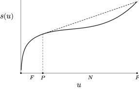
Figure 1: Schematic graph of $s(u)$, showing the set $F=(-\frac{1}{2},u_{0})\cup\{-\frac{1}{2q}\}$ of full ensemble equivalence, the singleton set $P=\{u_{0}\}$ of partial equivalence, and the set $N=(u_{0},-\frac{1}{2q})$ of nonequivalence. For $u\in F\cup P=(-\frac{1}{2},u_{0}]\cup\{-\frac{1}{2}\}$, $s(u)=s^{**}(u)$; for $u\in N$, $s(u)<s^{**}(u)$ and the graph of $s^{**}$ consists of the dotted line segment with slope $\beta_{c}$. The slope of $s$ at $-\frac{1}{2}$ is $\infty$.

According to Figure 1 and Theorem 5.1, there exists $u_{0}\in(-\frac{1}{2},-\frac{1}{2q})$ with the following properties.

• $s$ is strictly concave on the interval $(-\frac{1}{2},u_{0})$ and at the point $-\frac{1}{2q}$. Hence for $u\in F=(-\frac{1}{2},u_{0})\cup\{-\frac{1}{2q}\}$ the ensembles are fully equivalent [Thm. 5.1(a)(i)]. In fact, for $u\in(-\frac{1}{2},u_{0})$, ${\cal E}^{u}={\cal E}_{\beta}$ with $\beta$ given by the thermodynamic formula $\beta=s^{\prime}(u)$.

• $s$ is concave but not strictly concave at $u_{0}$ and has a nonstrictly supporting line at $u_{0}$ that also touches the graph of $s$ over the right hand endpoint $-\frac{1}{2q}$. Hence for $u=u_{0}$ the ensembles are partially equivalent in the sense that there exists $\beta\in I\!\!R$ such that ${\cal E}^{u}\subset{\cal E}_{\beta}$ but ${\cal E}^{u}\not={\cal E}_{\beta}$ [Thm. 5.1(a)(ii)]. In fact, $\beta$ equals the critical inverse temperature $\beta_{c}$ defined in (3.1).

• $s$ is not concave on the interval $N=(u_{0},-\frac{1}{2q})$ and has no supporting line at any $u\in N$ (CosEllTouTur, , Thm. A.4(c)). Hence for $u\in N$ the ensembles are nonequivalent in the sense that for all $\beta\in I\!\!R$, ${\cal E}^{u}\cap{\cal E}_{\beta}=\emptyset$ [Thm. 5.1(a)(iii)].

We point out two additional features of Figure 1. First, although ${\cal E}^{u}\not=\emptyset$ for $u$ equal to the right hand endpoint $-\frac{1}{2}$ of $\mbox{dom}\,s$, we do not include this point in the set $F$ of full ensemble equivalence. Indeed, $s$ is not strictly concave at $-\frac{1}{2}$ because there is no strictly supporting line at $-\frac{1}{2}$; as one can see in (5.1), the slope of $s$ at $-\frac{1}{2}$ is $\infty$. Nevertheless, by introducing the limiting set

$${\cal E}_{\infty}=\{(1,0,\ldots,0),(0,1,\ldots,0),\ldots,(0,0,\ldots,1)\}=\lim_{\beta\rightarrow\infty}{\cal E}_{\beta},$$

we can extend full ensemble equivalence to $u=-\frac{1}{2}$ since ${\cal E}^{-\frac{1}{2}}={\cal E}_{\infty}$.

Second, for $u$ in the interval $N$ of ensemble nonequivalence, the graph of $s^{**}$ is affine; this is depicted by the dotted line segment in Figure 1. The slope of the affine portion of the graph of $s^{**}$ equals the critical inverse temperature $\beta_{c}$ defined in (3.1). This can be proved using concave-duality relationships involving $s^{**}$ and the canonical free energy. The quantity $\beta_{c}$ also satisfies an equal-area property, first observed by Maxwell (Huang, , p. 45) and explained in the context of another spin model in (EllTouTur, , p. 535).

The relationships stated in the three bulleted items above give valuable insight into equivalence and nonequivalence of ensembles in the Curie-Weiss-Potts model. These relationships are illustrated in Figure 2. In this figure we exhibit the graph of $s^{\prime}$ and the sets ${\cal E}_{\beta}$ and ${\cal E}^{u}$ in order to compare the phase transitions in the two ensembles and to understand the implications for ensemble equivalence and nonequivalence. In order to accentuate properties of $s^{\prime}$, ${\cal E}_{\beta}$, and ${\cal E}^{u}$ that are related to ensemble equivalence and nonequivalence, we focus on $q=8$. In presenting the graph of $s^{\prime}$ and the form of ${\cal E}^{u}$, we assume that for $q=8$ Conjecture 4.1 is valid. We then appeal to part (c) of Theorem 4.3, which gives an explicit formula for $s$, and to part (d) of Theorem 4.2, which gives an explicit formula for the elements of ${\cal E}^{u}$. The derivative $s^{\prime}$, graphed in the top left plot in Figure 2, is given by

$$s^{\prime}(u)=\sqrt{\frac{q-1}{-2qu-1}}\left[\log\!\left(1+\sqrt{(q-1)(-2qu-1)}\,\,\right)-\log\!\left(1-\sqrt{\frac{-2qu-1}{q-1}}\,\right)\right].$$ (5.1)

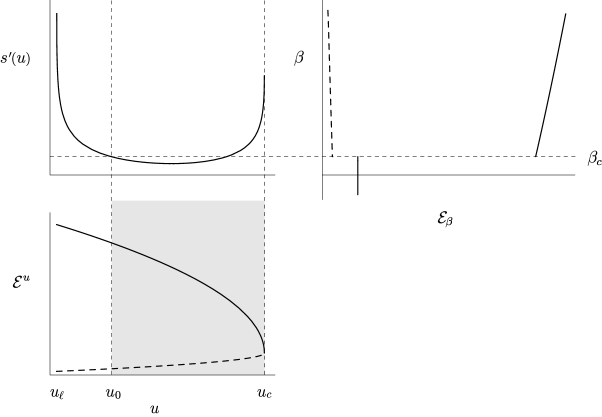
Figure 2: For $q=8$ the top right plot shows ${\cal E}_{\beta}$, the top left plot the graph of $s^{\prime}(u)$ for $u\in\mbox{dom}\,s=[u_{\ell},u_{c}]=[-\frac{1}{2},-\frac{1}{2q}]$, and the bottom left plot ${\cal E}^{u}$. The discontinuous phase transition at $\beta_{c}$ in the top right plot and the continuous phase transition at $u_{c}$ in the bottom left plot imply that the ensembles are nonequivalent for all $u\in N=(u_{0},u_{c})$. On this interval $s$ is not concave and $s^{**}$ is affine with slope $\beta_{c}$. The shaded area in the bottom left plot corresponds to the region of nonequivalence of ensembles delineated by $u\in N$.

The canonical phase diagram, given in the top right plot in Figure 2, summarizes the description of ${\cal E}_{\beta}$ given in Theorem 3.1 and shows the discontinuous phase transition exhibited by this ensemble at $\beta_{c}=\frac{2(q-1)}{q-2}\log(q-1)=\frac{7}{3}\log 7$. The solid line in this plot for $\beta<\beta_{c}$ represents the common value $\frac{1}{8}$ of each of the components of $\rho$, which is the unique phase for $\beta<\beta_{c}$. For $\beta>\beta_{c}$ there are eight phases given by $\nu^{1}(\beta)$ together with the vectors $\nu^{i}(\beta)$ obtained by interchanging the first and $i$th components of $\nu^{1}(\beta)$. Finally, for $\beta=\beta_{c}$ there are nine phases consisting of $\rho$ and the vectors $\nu^{i}(\beta_{c})$ for $i=1,2,\ldots,8$. The solid and dashed curves in the top right plot in Figure 2 show the first component and the last seven, equal components of $\nu^{1}(\beta)$ for $\beta\in[\beta_{c},\infty)$. The first component is a strictly increasing function equal to $\frac{7}{8}$ for $\beta=\beta_{c}$ and increasing to $1$ as $\beta\rightarrow\infty$ while the last seven, equal components are strictly decreasing functions equal to $\frac{1}{56}$ for $\beta=\beta_{c}$ and decreasing to $0$ as $\beta\rightarrow\infty$.

The microcanonical phase diagram, given in the bottom left plot in Figure 2, summarizes the description of ${\cal E}^{u}$ given in Theorem 4.2 and shows the continuous phase transition exhibited by this ensemble as $u$ decreases from the maximum value $u_{c}=-\frac{1}{2q}=-\frac{1}{16}$. The single phase $\rho$ for $u=-\frac{1}{16}$ is represented by the point lying over this value of $u$. For $u\in[-\frac{1}{2},-\frac{1}{16})$ there are eight phases given by $\nu^{1}(u)$ together with the vectors $\nu^{i}(u)$ obtained by interchanging the first and $i$th components of $\nu^{1}(u)$. The solid and dashed curves in the bottom left plot in Figure 2 show the first component $a(u)$ and the last seven, equal components $b(u)$ of $\nu^{1}(u)$ for $u\in[-\frac{1}{2},-\frac{1}{16})$. The first component is a strictly increasing function of $-u$ equal to $\frac{1}{8}$ for $u=-\frac{1}{16}$ and increasing to 1 as $u\rightarrow-\frac{1}{2}$, while the last seven, equal components are strictly decreasing functions of $-u$ equal to $\frac{1}{8}$ for $u=-\frac{1}{16}$ and decreasing to 0 as $u\rightarrow-\frac{1}{2}$.

The different nature of the two phase transitions — discontinuous in the canonical ensemble versus continuous in the microcanonical ensemble — implies that the two ensembles are not fully equivalent for all values of $u$. By necessity, the set ${\cal E}_{\beta}$ of canonical equilibrium macrostates must omit a set of microcanonical equilibrium macrostates. Further details concerning ensemble equivalence and nonequivalence can be seen by examining the graph of $s^{\prime}$, given in the top left plot of Figure 2. This graph, which is the bridge between the canonical and microcanonical phase diagrams, shows that $s^{\prime}$ is strictly decreasing on the interval $\mbox{int}\,F=(-\frac{1}{2},u_{0})$, which is the interior of the set $F$ of full ensemble equivalence. The critical value $\beta_{c}$ equals the slope of the affine portion of the graph of $s^{**}$ over the interval $N=(u_{0},-\frac{1}{2q})$ of ensemble nonequivalence. This affine portion is represented in the top left plot of Figure 2 by the horizontal dashed line at $\beta_{c}$.

Figure 2 exhibits the full equivalence of ensembles that holds for $u\in\mbox{int}\,F=(-\frac{1}{2},u_{0})$ [Thm. 6.2(a)]. For $u$ in this interval the solid and dashed curves representing the components of $\nu^{1}(u)\in{\cal E}^{u}$ can be put in one-to-one correspondence with the solid and dashed curves representing the same two components of $\nu^{1}(\beta)\in{\cal E}_{\beta}$ for $\beta\in(\beta_{c},\infty)$. The values of $u$ and $\beta$ are related by $s^{\prime}(u)=\beta$. Full equivalence of ensembles also holds for $u=-\frac{1}{2q}\in F$, the right-hand endpoint of the interval on which $s$ is finite. The solid vertical line in the top right plot for $\beta<\beta_{c}$, which represents the unique phase $\rho$, is collapsed to the single point representing the unique phase $\rho$ for $u=-\frac{1}{2q}$ in the bottom left plot. This collapse shows that the canonical notion of temperature is somewhat ill-defined at $u=-\frac{1}{2q}$ since lowering $\beta$ down to $\beta_{c}$ changes neither the equilibrium macrostate $\rho$ nor the associated mean energy $u$. This feature of the Curie-Weiss-Potts model is not present, for example, in the mean-field Blume-Emery-Griffiths spin model, which also exhibits nonequivalence of ensembles EllTouTur .

By comparing the top right and bottom left plots, we see that the elements of ${\cal E}^{u}$ cease to be related to those of ${\cal E}_{\beta}$ for $u\in N=(u_{0},-\frac{1}{2q})$, which is the interval on which $s$ is not concave. For any mean-energy value $u$ in this interval no $\nu\in{\cal E}_{\beta}$ exists that can be put in correspondence with an equivalent equilibrium empirical vector contained in $\mathcal{E}^{u}$. Thus, although the equilibrium macrostates corresponding to $u\in N$ are characterized by a well defined value of the mean energy, it is impossible to assign an inverse temperature $\beta$ to those macrostates from the viewpoint of the canonical ensemble. In other words, the canonical ensemble is blind to all mean-energy values $u$ contained in the interval $N$ of nonconcavity of $s$. This is closely related to the presence of the discontinuous phase transition seen in the canonical ensemble.

The quantity $u_{0}$ defined in (6.2) plays a central role in the analysis of phase transitions and ensemble equivalence in the Curie-Weiss-Potts model. First, as we saw in our discussion of Figure 1, $u_{0}$ separates the interval $(-\frac{1}{2},u_{0})$ of full ensemble equivalence from the interval $(u_{0},-\frac{1}{2q})$ of nonequivalence. Second, part (a) of Lemma 6.1 shows that $u_{0}$ equals the limiting mean energy $\tilde{H}(\nu^{1}(\beta_{c}))$ in the canonical equilibrium macrostate $\nu^{1}(\beta)$ as $\beta\rightarrow(\beta_{c})^{+}$. In Figures 3 and 4 we present for $q=3$ a third, geometric interpretation of $u_{0}$ that is also related to nonequivalence of ensembles.

Before explaining this third, geometric interpretation of $u_{0}$, we recall that according to part (a) of Theorem 4.2, ${\cal E}^{u}$ is nonempty, or equivalently the constraint set in (4.5) is nonempty, if and only if $u\in[-\frac{1}{2},-\frac{1}{2q}]=[-\frac{1}{2},-\frac{1}{6}]$. Geometrically, the energy constraint $\tilde{H}(\nu)=-\frac{1}{2}\langle\nu,\nu\rangle=u$ corresponds to the sphere in $I\!\!R^{3}$ with center 0 and radius $\sqrt{-2u}$. This sphere intersects the set $\mathcal{P}$ of probability vectors if and only if $u\in[-\frac{1}{2},-\frac{1}{6}]$. For $u=-\frac{1}{6}$, the sphere is tangent to $\mathcal{P}$ at the unique point $\rho$ while for $u=-\frac{1}{2}$, the hypersphere intersects $\mathcal{P}$ at the $q$ unit-coordinate vectors. The intersection of the sphere and $\mathcal{P}$ undergoes a phase transition at $u_{0}$ in the following sense. For $u\in[u_{0},-\frac{1}{6})$ the sphere intersects $\mathcal{P}$ in a circle while for $u\in[-\frac{1}{2},u_{0})$, the sphere intersects $\mathcal{P}$ in a proper subset of a circle; the complement of this subset lies outside the nonnegative octant of $I\!\!R^{3}$. For $u=u_{0}=-\frac{1}{4}$, the circle of intersection is maximal and is tangent to the boundary of $\mathcal{P}$.

The set ${\cal E}_{\beta}$ of canonical equilibrium macrostates for $q=3$ is represented in Figure 3. In this figure the maximal circle of intersection corresponding to $u=u_{0}=-\frac{1}{4}$ is shown together with the vector $\rho$ at its center; the points $A$, $B$, and $C$ representing the respective unit-coordinate vectors $(1,0,0)$, $(0,1,0)$, and $(0,0,1)$; and the points $A_{c}$, $B_{c}$, and $C_{c}$ representing the respective equilibrium macrostates $\nu^{1}(\beta_{c})$, $\nu^{2}(\beta_{c})$, and $\nu^{3}(\beta_{c})$. These three macrostates lie on the maximal circle of intersection since $\tilde{H}(\nu^{1}(\beta_{c}))=u_{0}$ [Lem. 6.1(b)]. For $\beta>\beta_{c}$ all $\nu\in{\cal E}_{\beta}$ have two equal components, and as $\beta\rightarrow\infty$ these vectors converge to the unit-coordinate vectors $A$, $B$, and $C$. Hence for $\beta>\beta_{c}$ the equilibrium macrostates $\nu^{1}(\beta)$, $\nu^{2}(\beta)$, and $\nu^{3}(\beta)$ are represented by the open line segments $\overline{A_{c}A}$, $\overline{B_{c}B}$, and $\overline{C_{c}C}$.

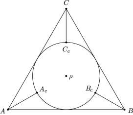
Figure 3: Graphical representation of the set ${\cal E}_{\beta}$ of canonical equilibrium macrostates for $q=3$ showing the maximal circle of intersection corresponding to $u=u_{0}$; the vector $\rho$ ; the unit-coordinate vectors $A$, $B$, and $C$; and the macrostates $A_{c}=\nu^{1}(\beta_{c})$, $B_{c}=\nu^{2}(\beta_{c})$, and $C_{c}=\nu^{3}(\beta_{c})$. The line segments $\overline{A_{c}A}$, $\overline{B_{c}B}$, and $\overline{C_{c}C}$ represent the elements of ${\cal E}_{\beta}$ for $\beta>\beta_{c}$.

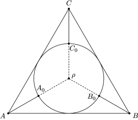
Figure 4: Graphical representation of the set ${\cal E}^{u}$ of microcanonical equilibrium macrostates for $q=3$ showing the maximal circle of intersection corresponding to $u=u_{0}$; the vector $\rho$ ; the unit-coordinate vectors $A$, $B$, and $C$; and the macrostates $A_{0}=\nu^{1}(u_{0})$, $B_{0}=\nu^{2}(u_{0})$, and $C_{0}=\nu^{3}(u_{0})$. The solid-line segments $\overline{A_{0}A}$, $\overline{B_{0}B}$, and $\overline{C_{0}C}$ represent the elements of ${\cal E}^{u}$ that are realized canonically. The dashed-line segments $\overline{\rho A_{0}}$, $\overline{\rho B_{0}}$, and $\overline{\rho C_{0}}$ represent the elements of ${\cal E}^{u}$ that are not realized canonically.

The set ${\cal E}^{u}$ of microcanonical equilibrium macrostates for $q=3$ is represented in Figure 4. In this figure the maximal circle of intersection corresponding to $u=u_{0}=-\frac{1}{4}$ is shown together with the vector $\rho$ at its center; the points $A$, $B$, and $C$ representing the unit-coordinate vectors; and the points $A_{0}$, $B_{0}$, and $C_{0}$ representing the respective equilibrium macrostates $\nu^{1}(u_{0})$, $\nu^{2}(u_{0})$, and $\nu^{3}(u_{0})$. For $u\in(-\frac{1}{2},-\frac{1}{6})$ all $\nu\in{\cal E}^{u}$ have two equal components, and as $u\rightarrow-\frac{1}{2}$ they converge to the unit coordinate vectors $A$, $B$, and $C$. Hence for $u\in(-\frac{1}{2},-\frac{1}{6})$ the equilibrium macrostates $\nu^{1}(u)$, $\nu^{2}(u)$, and $\nu^{3}(u)$ are represented by the open line segments $\overline{\rho A}$, $\overline{\rho B}$, and $\overline{\rho C}$. As we saw in the preceding section, for each $u\in(-\frac{1}{2},-\frac{1}{6})$ the macrostates $\nu^{1}(u)$, $\nu^{2}(u)$, and $\nu^{3}(u)$ lie on the intersection of the sphere of radius $\sqrt{-2u}$ with $\mathcal{P}$. In particular, $A_{0}=\nu^{1}(u_{0})$, $B_{0}=\nu^{2}(u_{0})$, and $C_{0}=\nu^{3}(u_{0})$ lie on the maximal circle of intersection.

The distinguishing feature of Figure 4 is the three open dashed-line segments $\overline{\rho A_{0}}$, $\overline{\rho B_{0}}$, and $\overline{\rho C_{0}}$ representing the elements of ${\cal E}^{u}$ that are not realized canonically; namely, $\nu^{1}(u)$, $\nu^{2}(u)$, and $\nu^{3}(u)$ for $u\in(u_{0},-\frac{1}{6})$. The three half open solid-line segments $\overline{A_{0}A}$, $\overline{B_{0}B}$, and $\overline{C_{0}C}$ represent the elements of ${\cal E}^{u}$ that are realized canonically; namely, $\nu^{1}(u)$, $\nu^{2}(u)$, and $\nu^{3}(u)$ for $u\in(-\frac{1}{2},u_{0}]$. For each such $u$ the value of $\beta$ for which ${\cal E}^{u}={\cal E}_{\beta}$ is determined by the equation $\tilde{H}(\nu^{1}(\beta))=u$ [Thm. 6.2(a)]. Thus in Figure 3 the corresponding elements of ${\cal E}_{\beta}$ lie on the intersection of the sphere of radius $\sqrt{-2u}$ and $\mathcal{P}$.

This completes our discussion of equivalence and nonequivalence of ensembles. In the next section we will prove a number of statements concerning ensemble equivalence and nonequivalence that have been determined graphically.

VI Proofs of Equivalence and Nonequivalence of Ensembles

Using the general results of EHT , we stated in the preceding section the equivalence and nonequivalence relationships that exist between ${\cal E}^{u}$ and ${\cal E}_{\beta}$ and verified these relationships using the plots of these sets for $q=8$ given in Figure 2. Our purpose in the present section is to prove these relationships using mapping properties of the mean energy function $u(\beta)$ defined for $\beta\not=\beta_{c}$ by

$$u(\beta)=\left\{\begin{array}[]{ll}\tilde{H}(\rho)=-\frac{1}{2q}&\ \mbox{ for }\>\beta<\beta_{c},\\ \tilde{H}(\nu^{1}(\beta))=-\frac{1}{2}\langle\nu^{1}(\beta),\nu^{1}(\beta)\rangle&\ \mbox{ for }\>\beta>\beta_{c}.\end{array}\right.$$ (6.1)

Here $\nu^{1}(\beta)$ is the unique canonical equilibrium macrostate modulo permutations for $\beta>\beta_{c}$ [Thm. 3.1]. According to the next lemma, for $\beta>\beta_{c}$, $u(\beta)$ is continuous and strictly decreasing and $u(\beta)<-\frac{1}{2q}$, which equals the mean energy for $\beta<\beta_{c}$. It follows that as $\beta$ increases through $\beta_{c}$, $u(\beta)$ is discontinuous, jumping down from $-\frac{1}{2q}$ to $\tilde{H}(\nu^{1}(\beta))$. This discontinuity in $u(\beta)$ mirrors in a natural way the discontinuity in ${\cal E}_{\beta}$ as $\beta$ increases through $\beta_{c}$.

Lemma 6.1

. For $\beta\in[\beta_{c},\infty)$ we define $\nu^{1}(\beta)$ as in part (b) of Theorem 3.1 and we define

$$u_{0}=\frac{-q^{2}+3q-3}{2q(q-1)},$$ (6.2)

The following conclusions hold.

(a) $-\frac{1}{2}<u_{0}<-\frac{1}{2q}$ and $\lim_{\beta\rightarrow(\beta_{c})^{+}}u(\beta)=\tilde{H}(\nu^{1}(\beta_{c}))=u_{0}$.

(b) The function mapping

$$\beta\in(\beta_{c},\infty)\mapsto u(\beta)=\tilde{H}(\nu^{1}(\beta))=-\textstyle\frac{1}{2}\langle\nu^{1}(\beta),\nu^{1}(\beta)\rangle$$

is a strictly decreasing, differentiable bijection onto the interval $(-\frac{1}{2},u_{0})$.

Proof. (a) The inequalities involving $u_{0}$ follow immediately from the inequality $q\geq 3$. The relationship $\tilde{H}(\nu^{1}(\beta_{c}))=u_{0}$ is easily determined using the explicit form of $\nu^{1}(\beta_{c})$ given in (3.5). That $\lim_{\beta\rightarrow(\beta_{c})^{+}}u(\beta)=\tilde{H}(\nu^{1}(\beta_{c}))$ follows from the definition of $u(\beta)$ and the continuity of $\nu^{1}(\beta)$ for $\beta>\beta_{c}$.

(b) For $\beta\in(\beta_{c},\infty)$ we use the formula for $\nu^{1}(\beta)$ given in part (b) of Theorem 3.1 to calculate

$$u(\beta)=-\frac{1}{2}\left(\frac{[1+(q-1)w(\beta)]^{2}}{q^{2}}+(q-1)\frac{[1-w(\beta)]^{2}}{q^{2}}\right).$$

Since $w(\beta)$ is positive, strictly increasing, and differentiable for $\beta\in(\beta_{c},\infty)$ [Thm. 3.1(a)] and since

$$u^{\prime}(\beta)=\frac{-(q-1)w(\beta)w^{\prime}(\beta)}{q}<0\ \mbox{ for }\beta\in(\beta_{c},\infty),$$

$u(\beta)$ is strictly decreasing for $\beta\in(\beta_{c},\infty)$. In addition, since $\lim_{\beta\rightarrow\infty}w(\beta)=1$ [Thm. 3.1(a)], we have $\lim_{\beta\rightarrow\infty}u(\beta)=-\frac{1}{2}$, and by part (a) of this lemma

$$\lim_{\beta\rightarrow(\beta_{c})^{+}}u(\beta)=\lim_{\beta\rightarrow(\beta_{c})^{+}}\tilde{H}(\nu(\beta_{c}))=u_{0}.$$

It follows that the function mapping $\beta\in(\beta_{c},\infty)\mapsto u(\beta)$ is a strictly decreasing, differentiable bijection onto the interval $(-\frac{1}{2},-\frac{1}{2}u_{0})$. This completes the proof of part (b).  

Mapping properties of $u(\beta)$ play an important role in the next theorem, in which we prove that the sets $F$, $P$, and $N$ defined in (6.3) correspond to full equivalence, partial equivalence, and nonequivalence of ensembles. For $u\in F$ we consider three subcases in order to indicate the value of $\beta$ for which ${\cal E}^{u}={\cal E}_{\beta}$; for $u\in\mbox{int}\,F=(-\frac{1}{2},u_{0})$, $\beta$ and $u$ are related by $\beta=s^{\prime}(u)$ and $u=u(\beta)$. Part (c) shows an interesting degeneracy in the equivalence-of-ensemble picture, the set ${\cal E}^{u}$ for $u=-\frac{1}{2q}$ corresponding to all ${\cal E}_{\beta}$ for $\beta<\beta_{c}$. This is related to the fact that for all such values of $\beta$, ${\cal E}_{\beta}=\{\rho\}$ and thus the mean energy $u(\beta)$ equals $-\frac{1}{2q}$.

Theorem 6.2

. We define $s(u)$ in (4.2), $u(\beta)$ in (6.1), ${\cal E}_{\beta}$ in (2.3), and ${\cal E}^{u}$ in (2.4). We also define $\beta_{c}$ in (3.1) and $u_{0}$ in (6.2). The sets

$$F=(\textstyle-\frac{1}{2},u_{0})\cup\{\textstyle-\frac{1}{2q}\},\ P=\{\textstyle u_{0}\},\ \mbox{ and }N=(\textstyle-\frac{1}{2}u_{0},-\frac{1}{2q})$$ (6.3)

have the following properties.

(a) Full equivalence on int $F$. For $u\in\mbox{{\em int}}\,F=(-\frac{1}{2},u_{0})$, there exists a unique $\beta\in(\beta_{c},\infty)$ such that ${\cal{E}}^{u}={\cal{E}}_{\beta}$; $\beta$ satisfies $u(\beta)=\tilde{H}(\nu^{1}(\beta))=u$.

(b) For $u\in\mbox{{\em int}}\,F=(-\frac{1}{2},u_{0})$, $s$ is differentiable. The values $u$ and $\beta$ for which ${\cal E}^{u}={\cal E}_{\beta}$ in part (a) are also related by the thermodynamic formula $s^{\prime}(u)=\beta$.

(c) Full equivalence at $-\frac{1}{2q}$. For $u=-\frac{1}{2q}\in F$, ${\cal E}^{-\frac{1}{2q}}={\cal E}_{\beta}$ for any $\beta<\beta_{c}$.

(d) Partial equivalence on $P$. For $u\in P=\{u_{0}\}$, ${\cal{E}}^{u_{0}}\subset{\cal{E}}_{\beta_{c}}$ but ${\cal{E}}^{u_{0}}\not={\cal{E}}_{\beta_{c}}$. In fact, ${\cal{E}}_{\beta_{c}}={\cal{E}}^{u_{0}}\cup{\cal E}^{-\frac{1}{2q}}$.

(e) Nonequivalence on $N$. For any $u\in N=(u_{0},-\frac{1}{2q})$, ${\cal{E}}^{u}\cap{\cal{E}}_{\beta}=\emptyset$ for all $\beta\in I\!\!R$.

In reference to the properties of $s$ given in part (b), one can show that the function mapping $u\in(-\frac{1}{2},u_{0})\mapsto s^{\prime}(u)$ is a strictly decreasing, differentiable bijection onto the interval $(\beta_{c},\infty)$ and that this bijection is the inverse of the bijection mapping $\beta\in(\beta_{c},\infty)\mapsto u(\beta)$.

Before we prove the theorem, it is instructive to compare its assertions with those in Theorem 5.1, which formulates ensemble equivalence and nonequivalence in terms of support properties of $s$. These support properties can be seen in the schematic plot of the the graph of $s$ in Figure 1. We start with part (a) of Theorem 6.2, which states that for any $u\in\mbox{int}\,F=(-\frac{1}{2},u_{0})$ there exists a unique $\beta\in(\beta_{c},\infty)$ such that ${\cal E}^{u}={\cal E}_{\beta}$. As promised in part (a)(i) of Theorem 5.1, this $\beta$ is the slope of a strictly supporting line to the graph of $s$ at $u$. The situation that holds when $u=-\frac{1}{2q}$ [Thm. 6.2(c)] is also consistent with part (a)(i) of Theorem 5.1. For this value of $u$, which is the isolated point of the set $F$ of full equivalence, there exist infinitely many strictly supporting lines to the graph of $s$, the possible slopes of which are all $\beta\in(-\infty,\beta_{c})$. On the other hand, when $u=u_{0}$, which is the only value lying in the set $P$ of partial equivalence, we have ${\cal{E}}^{u_{0}}\subset{\cal{E}}_{\beta_{c}}$ but ${\cal{E}}^{u_{0}}\not={\cal{E}}_{\beta_{c}}$ [Thm. 6.2(d)]. In combination with part (a)(ii) of Theorem 5.1, it follows that there exists a nonstrictly suppporting line at $u$ with slope $\beta_{c}$. Finally, for $u\in N=(u_{0},-\frac{1}{2q})$, we have ${\cal E}^{u}\cap{\cal E}_{\beta}=\emptyset$ for all $\beta\in I\!\!R$ [Thm. 6.2(e)]. In accordance with part (a)(iii) of Theorem 5.1, $s$ has no supporting line at any $u\in N$, and by Theorem A.4 in CosEllTouTur $s$ is not concave at any $u\in N$.

Proof of Theorem 6.2. (a) For $\beta>\beta_{c}$ part (b) of Theorem 3.1 and part (b) of Theorem 5.1 imply that

$${\cal{E}}_{\beta}=\{\nu^{1}(\beta),\ldots,\nu^{q}(\beta)\}=\bigcup_{u\in\tilde{H}({\cal{E}}_{\beta})}{\cal{E}}^{u}.$$

The symmetry of $\tilde{H}$ with respect to permutations implies that $\tilde{H}({\cal{E}}_{\beta})=\{\tilde{H}(\nu^{1}(\beta))\}$. Thus for any $\beta>\beta_{c}$

$${\cal{E}}_{\beta}={\cal{E}}^{\tilde{H}(\nu^{1}(\beta))}.$$ (6.4)

Since for any $u\in\mbox{int}\,F=(-\frac{1}{2},u_{0})$ there exists a unique $\beta\in(\beta_{c},\infty)$ satisfying $u(\beta)=\tilde{H}(\nu^{1}(\beta))=u$ [Lem. 6.1(b)], it follows that ${\cal E}^{u}={\cal E}_{\beta}$.

(b) According to part (b) of Theorem 6.3, $s$ is differentiable at all $u\in\mbox{int}\,F$. Since $s=s^{**}$ in a neighborhood of each such $u$, part (a) of Theorem A.3 in CosEllTouTur implies that $s^{\prime}(u)=\beta$.

(c) By (4.6) and part (b) of Theorem 3.1

$${\cal E}^{-\frac{1}{2q}}=\{\rho\}={\cal E}_{\beta}\ \mbox{ for any }\beta<\beta_{c}.$$ (6.5)

(d) By part (b) of Theorem 3.1, symmetry, and part (a) of Lemma 6.1

$$\tilde{H}({\cal{E}}_{\beta_{c}})=\{\tilde{H}(\rho),\tilde{H}(\nu^{1}(\beta_{c}))\}=\{\textstyle-\frac{1}{2q},u_{0}\}.$$

Hence by (6.4) and (6.5)

$${\cal E}_{\beta_{c}}=\bigcup_{u\in\tilde{H}({\cal{E}}_{\beta_{c}})}{\cal E}^{u}={\cal E}^{-\frac{1}{2q}}\cup{\cal E}^{u_{0}}=\{\rho\}\cup{\cal E}^{u_{0}}.$$

However, $\rho\notin{\cal{E}}^{u_{0}}$ since $\rho$ does not satisfy the constraint $\tilde{H}(\rho)=u_{0}$. It follows that ${\cal{E}}^{u_{0}}\subset{\cal{E}}_{\beta_{c}}$ but that ${\cal{E}}^{u_{0}}\not={\cal{E}}_{\beta_{c}}$.

(e) If $u\in N$, then $u\notin(-\frac{1}{2},u_{0})$, and so by part (a) of Lemma 6.1 $u\not=\tilde{H}(\nu^{1}(\beta))$ for any $\beta\in(\beta_{c},\infty)$. Since by (6.4) ${\cal{E}}_{\beta}={\cal{E}}^{\tilde{H}(\nu^{1}(\beta))}$ for all $\beta>\beta_{c}$, it follows that for all $\beta>\beta_{c}$

$${\cal{E}}^{u}\cap{\cal{E}}^{\tilde{H}(\nu^{1}(\beta))}=\emptyset$$

and thus that ${\cal{E}}^{u}\cap{\cal{E}}_{\beta}=\emptyset$. For any $\beta<\beta_{c}$ (6.5) states that ${\cal E}_{\beta}={\cal E}^{-\frac{1}{2q}}=\{\rho\}$. Since $u\in N$, we have $u\not=-\frac{1}{2q}$ and thus ${\cal E}^{-\frac{1}{2q}}\cap{\cal E}^{u}=\emptyset$. It follows that ${\cal{E}}^{u}\cap{\cal{E}}_{\beta}=\emptyset$ for any $\beta<\beta_{c}$. Finally, for $\beta=\beta_{c}$ part (b) of Theorem 3.1 states that ${\cal E}_{\beta_{c}}=\{\rho,\nu^{1}(\beta_{c}),\ldots,\nu^{q}(\beta_{c})\}$. However, since $\tilde{H}(\rho)=-\frac{1}{2q}\notin N$ and $\tilde{H}(\nu^{i}(\beta_{c}))=u_{0}\notin N$, none of the vectors in ${\cal E}_{\beta_{c}}$ satisfies the constraint $\tilde{H}(\nu)=u$ . Thus ${\cal{E}}^{u}\cap{\cal{E}}_{\beta_{c}}=\emptyset$. We have proved ${\cal{E}}^{u}\cap{\cal{E}}_{\beta}=\emptyset$ for all $\beta\in I\!\!R$. The proof of the theorem is complete.   

We end this section by showing that for arbitrary $q\geq 4$ and $u$ in the equivalence sets $F\cup P=(-\frac{1}{2},u_{0}]\cup\{-\frac{1}{2q}\}$ the formulas for ${\cal E}^{u}$ and $s(u)$ given in part (d) of Theorem 4.2 and part (c) of Theorem 4.3 are rigorously true. Our strategy is to use the equivalence of the microcanonical and canonical ensembles for $u\in F\cup P$ and the fact that the form of ${\cal E}_{\beta}$ is known exactly for all $\beta$. Thus, we translate the form of $\nu\in{\cal E}_{\beta}$, as given in part (b) of Theorem 3.1, into the form of $\nu\in{\cal E}^{u}$ for $u\in F\cup P$. For $\beta\in[\beta_{c},\infty)$, the last $q-1$ components of $\nu^{1}(\beta)\in{\cal E}_{\beta}$ are given by

$$\nu^{1}_{j}(\beta)=\frac{1-w(\beta)}{q},$$ (6.6)

and these components are not equal to the first component. Since for each $u\in F\cup P$ there exists $\beta\in[\beta_{c},\infty]$ such that either ${\cal{E}}^{u}={\cal{E}}_{\beta}$ or ${\cal E}^{u}\subset{\cal E}_{\beta}$, it follows that modulo permutations all $\nu\in{\cal{E}}^{u}$ have their last $q-1$ components equal to each other. That is, modulo permutations there exist numbers $a$ and $b$ in $[0,1]$ such that $\nu=(a,b,\ldots,b)$. The possible values of $a$ and $b$ are easily determined by considering the constraints satisfied by $\nu\in{\cal E}^{u}$. These constraints are

$$a+(q-1)b=1\ \mbox{ and }\ a^{2}+(q-1)b^{2}=-2u.$$

The two solutions of these equations are

$$a_{1}=\frac{1-\sqrt{(q-1)(-2qu-1)}}{q},\ \ b_{1}=\frac{q-1+\sqrt{(q-1)(-2qu-1)}}{(q-1)q}$$

and

$$a_{2}=\frac{1+\sqrt{(q-1)(-2qu-1)}}{q},\ \ b_{2}=\frac{q-1-\sqrt{(q-1)(-2qu-1)}}{(q-1)q}.$$

Of the two values $b_{1}$ and $b_{2}$, only $b_{2}$ has the form given in (6.6) with

$$w(\beta)=\frac{\sqrt{(q-1)(-2qu-1)}}{q-1}\in[0,1].$$

We conclude that modulo permutations each $\nu\in{\cal E}^{u}$ has the form $(a_{2},b_{2},\ldots,b_{2})$, in which the last $q-1$ components all equal $b_{2}$. This coincides with the formula for $\nu^{1}(u)$ given in part (d) of Theorem 4.2, which in turn gives the explicit formula for $s(u)$ in part (c) of Theorem 4.3. This information is summarized in part (a) of the next theorem. The differentiability of $s$ on $\mbox{int}\,F$, which is stated in part (b), is an immediate consequence of the explicit formula for $s(u)$.

Theorem 6.3

. We define $u_{0}$ in (6.2). The following conclusions hold.

(a) For arbitrary $q\geq 4$ and $u$ in the equivalence sets $F\cup P=(-\frac{1}{2},u_{0}]\cup\{-\frac{1}{2q}\}$ the formulas for ${\cal E}^{u}$ and $s(u)$ given in part (d) of Theorem 4.2 and part (c) of Theorem 4.3 are rigorously true.

(b) For arbitrary $q\geq 4$, $s$ is differentiable on the interval $\mbox{{\em int}}\,F=(-\frac{1}{2},u_{0})$ and $s^{\prime}(u)$ is given by (5.1).

Appendix A Two Related Maximization Problems

Theorem A.1 is a new result on the maximum points of certain functions related by convex duality. It is formulated for a finite, differentiable, convex function $F$ on $I\!\!R^{\sigma}$ and its Legendre-Fenchel transform

$$F^{*}(z)=\sup_{x\in I\!\!R^{\sigma}}\{\langle x,z\rangle-F(x)\}.$$

With only minor changes in notation the theorem is also valid for a finite, Gateaux-differentiable, convex function on a Hilbert space.

Theorem A.1 will be applied in Appendix B to prove that for $\beta>0$, ${\cal E}_{\beta}$ has the form given in part (b) of Theorem 3.1. Another application of Theorem A.1 is given in Proposition 3.4 in EllOttTou . It is used there to determine the form of the set of canonical equilibrium macrostates for another important spin system known as the mean-field Blume-Emery-Griffiths model.

Theorem A.1

. Let $\sigma$ be a positive integer and $F$ a finite, differentiable, convex function mapping $I\!\!R^{\sigma}$ into $I\!\!R$. Assume that $\sup_{z\in I\!\!R^{\sigma}}\{F(z)-\frac{1}{2}\|z\|^{2}\}<\infty$ and that $F(z)-\frac{1}{2}\|z\|^{2}$ attains its supremum. The following conclusions hold.

(a) $\sup\limits_{z\in I\!\!R^{\sigma}}\{F(z)-\frac{1}{2}\|z\|^{2}\}=\sup\limits_{z\in\mbox{{\scriptsize\rm dom}}\,F^{*}}\{\frac{1}{2}\|z\|^{2}-F^{*}(z)\}$.

(b) $\frac{1}{2}\|z\|^{2}-F^{*}(z)$ attains its supremum on $\mbox{{\em dom}}\,F^{*}$.

(c) The global maximum points of $F(z)-\frac{1}{2}\|z\|^{2}$ coincide with the global maximum points of $\frac{1}{2}\|z\|^{2}-F^{*}(z)$.

Proof. We define the subdifferential of $F^{*}$ at $z_{0}\in I\!\!R^{\sigma}$ by

$$\partial F^{*}(z_{0})=\{y\in I\!\!R^{\sigma}:F^{*}(z)\geq F^{*}(z_{0})+\langle y,z-z_{0}\rangle\mbox{ for all }z\in I\!\!R^{\sigma}\}.$$

We also define the domain of $\partial F^{*}$ to be the set of $z_{0}\in I\!\!R^{\sigma}$ for which $\partial F^{*}(z_{0})\not=\emptyset$. The proof of the theorem uses three properties of Legendre-Fenchel transforms.

1. $F^{*}$ is a convex, lower semicontinuous function mapping $I\!\!R^{\sigma}$ into $I\!\!R\cup\{\infty\}$, and for all $z\in I\!\!R^{\sigma}$, $F^{**}(z)=(F^{*})^{*}(z)$ equals $F(z)$ (Ellis, , Thm. VI.5.3(a),(e)).

2. If for some $z_{0}\in I\!\!R^{\sigma}$ and $z\in I\!\!R^{\sigma}$ we have $z=\nabla F(z_{0})$, then $F(z_{0})+F^{*}(z)=\langle z_{0},z\rangle$, and so $z\in\mbox{dom}\,F^{*}$. In particular, if $z=z_{0}$, then $z_{0}\in\mbox{dom}\,F^{*}$ and $F(z_{0})+F^{*}(z_{0})=\|z_{0}\|^{2}$.

3. For $z_{0}\in\mbox{dom}\,F^{*}$ and $y\in\partial F^{*}(z_{0})$ we have $F(y)+F^{*}(z_{0})=\langle y,z_{0}\rangle$ (Ellis, , Thm. VI.5.3(c),(d)). In particular, if $y=z_{0}$, then $F(z_{0})+F^{*}(z_{0})=\|z_{0}\|^{2}$.

We first prove part (a), which is a special case of Theorem C.1 in EE . Let $M=\sup_{z\in I\!\!R^{\sigma}}\{F(z)-\|z\|^{2}/2\}$. Since for any $z\in\mbox{dom}\,F^{*}$ and $x$ in $I\!\!R^{\sigma}$

$$F^{*}(z)+M\geq\langle x,z\rangle-F(x)+M\geq\langle x,z\rangle-\|x\|^{2}/2,$$

we have

$$F^{*}(z)+M\geq\sup_{x\in I\!\!R^{\sigma}}\{\langle x,z\rangle-\|x\|^{2}/2\}=\|z\|^{2}/2.$$

It follows that $M\geq\|z\|^{2}/2-F^{*}(z)$ and thus that $M\geq\sup_{z\in\mbox{{\scriptsize\rm dom}}\,F^{*}}\{\|z\|^{2}/2-F^{*}(z)\}$. To prove the reverse inequality, let $N=\sup_{z\in\mbox{{\scriptsize\rm dom}}\,F^{*}}\{\|z\|^{2}/2-F^{*}(z)\}$. Then for any $z\in I\!\!R^{\sigma}$ and $x\in\mbox{dom}\,F^{*}$

$$\|z\|^{2}/2+N\geq\langle x,z\rangle-\|x\|^{2}/2+N\geq\langle x,z\rangle-F^{*}(x).$$

Since $F^{*}(x)=\infty$ for $x\not\in\mbox{dom}\,F^{*}$, it follows from property 1 that

$$\|z\|^{2}/2+N\geq\sup_{x\in\mbox{{\scriptsize\rm dom}}\,F^{*}}\{\langle x,z\rangle-F^{*}(x)\}=F(z)$$

and thus that $N\geq\sup_{z\in I\!\!R^{\sigma}}\{F(z)-\|z\|^{2}/2\}$.

In order to prove parts (b) and (c) of Theorem A.1, let $z_{0}$ be any point in $I\!\!R^{\sigma}$ at which $F(z)-\frac{1}{2}\|z\|^{2}$ attains its supremum. Then $z_{0}=\nabla F(z_{0})$, and so by the last line of property 2, $z_{0}\in\mbox{dom}\,F^{*}$ and $F(z_{0})+F^{*}(z_{0})=\|z_{0}\|^{2}$. Part (a) now implies that

$$\sup_{z\in I\!\!R^{\sigma}}\{F(z)-\textstyle\frac{1}{2}\|z\|^{2}\} = F(z_{0})-\textstyle\frac{1}{2}\|z_{0}\|^{2}$$

$$= \textstyle\frac{1}{2}\|z_{0}\|^{2}-F^{*}(z_{0})=\displaystyle\sup_{z\in\mbox{{\scriptsize\rm dom}}\,F^{*}}\{\textstyle\frac{1}{2}\|z\|^{2}-F^{*}(z)\}.$$

We conclude that $\frac{1}{2}\|z\|^{2}-F^{*}(z)$ attains its supremum on $\mbox{dom}\,F^{*}$ at $z_{0}$. Not only have we proved part (b), but also we have proved half of part (c); namely, any global maximizer of $F(z)-\frac{1}{2}\|z\|^{2}$ is a global maximizer of $\frac{1}{2}\|z\|^{2}-F^{*}(z)$.

Now let $z_{0}$ be any point at which $\frac{1}{2}\|z\|^{2}-F^{*}(z)$ attains its supremum. Then for any $z\in I\!\!R^{\sigma}$

$$\textstyle\frac{1}{2}\langle z_{0},z_{0}\rangle-F^{*}(z_{0})\geq\textstyle\frac{1}{2}\langle z,z\rangle-F^{*}(z).$$

It follows that for any $z\in I\!\!R^{\sigma}$

$$F^{*}(z)\geq F^{*}(z_{0})+\textstyle\frac{1}{2}(\langle z,z\rangle-\langle z_{0},z_{0}\rangle)\geq F^{*}(z_{0})+\langle z_{0},z-z_{0}\rangle$$

and thus that $z_{0}\in\partial F^{*}(z_{0})$. By the last line of property 3 this implies that $F(z_{0})+F^{*}(z_{0})=\|z_{0}\|^{2}$. In conjunction with part (a) this in turn implies that

$$\sup_{z\in\mbox{{\scriptsize dom}}\,F^{*}}\{\textstyle\frac{1}{2}\|z\|^{2}-F^{*}(z)\} = \textstyle\frac{1}{2}\|z_{0}\|^{2}-F^{*}(z_{0})$$

$$= F(z_{0})-\textstyle\frac{1}{2}\|z_{0}\|^{2}=\displaystyle\sup_{z\in I\!\!R^{\sigma}}\{\textstyle F(z)-\frac{1}{2}\|z\|^{2}\}.$$

We conclude that $F(z)-\frac{1}{2}\|z\|^{2}$ attains its supremum at $z_{0}$. This completes the proof of the theorem.     

Appendix B Form of ${\cal E}_{\beta}$

We first derive the form of ${\cal E}_{\beta}$ for $\beta>0$ as given in part (b) of Theorem 3.1. We then prove that ${\cal E}_{\beta}=\{\rho\}$ for all $\beta\leq 0$.

${\cal E}_{\beta}$ is defined as the set of $\nu\in\mathcal{P}$ that minimize $R(\nu|\rho)-\frac{\beta}{2}\langle\nu,\nu\rangle$. Since $\beta>0$, this is equivalent to

$${\cal E}_{\beta}=\left\{\nu\in\mathcal{P}:\nu\mbox{ maximizes }\textstyle\frac{1}{2}\langle\nu,\nu\rangle-\textstyle\frac{1}{\beta}R(\nu|\rho)\right\}.$$ (B.1)

This maximization problem has the form of the right hand side of part (a) of Theorem A.1; viz.,

$$\sup_{\nu\in\mathcal{P}}\left\{\textstyle\frac{1}{2}\langle\nu,\nu\rangle-\textstyle\frac{1}{\beta}R(\nu|\rho)\right\}=\sup_{\nu\in\mbox{\scriptsize dom}\,F^{*}}\{\textstyle\frac{1}{2}\|\nu\|^{2}-F^{*}(\nu)\}$$

with $F^{*}(\nu)=\frac{1}{\beta}R(\nu|\rho)$. For $z\in I\!\!R^{q}$ we define the finite, convex, continuous function

$$\Gamma(z)=\textstyle\log\left(\sum_{i=1}^{q}e^{z_{i}}\,\frac{1}{q}\right).$$ (B.2)

Since for $\nu\in I\!\!R^{q}$ (Ellis, , Thm. VIII.2.2)

$$(\Gamma)^{*}(\nu)=\left\{\begin{array}[]{ll}R(\nu|\rho)&\>\mbox{ for }\nu\in\mathcal{P}\\ \infty&\>\mbox{ otherwise },\end{array}\right.$$

it follows that for $z\in I\!\!R^{q}$

$$F(z)=\sup_{\nu\in\mathcal{P}}\left\{\langle z,\nu\rangle-\textstyle\frac{1}{\beta}R(\nu|\rho)\right\}=\textstyle\frac{1}{\beta}\displaystyle\sup_{\nu\in\mathcal{P}}\left\{\langle\beta z,\nu\rangle-R(\nu|\rho)\right\}=\textstyle\frac{1}{\beta}\Gamma(\beta z).$$

Thus by part (a) of Theorem A.1

$$\sup_{z\in I\!\!R^{q}}\left\{\textstyle\frac{1}{\beta}\Gamma(\beta z)-\textstyle\frac{1}{2}\|z\|^{2}\right\}=\sup_{\nu\in\mathcal{P}}\left\{\textstyle\frac{1}{2}\langle\nu,\nu\rangle-\textstyle\frac{1}{\beta}R(\nu|\rho)\right\},$$

and by part (b) of the theorem the global maximum points of the two functions coincide.

Equation (B.1) now implies that

$${\cal E}_{\beta} = \left\{z\in I\!\!R^{q}:z\mbox{ maximizes }\textstyle\frac{1}{\beta}\Gamma(\beta z)-\textstyle\frac{1}{2}\|z\|^{2}\right\}$$

$$= \left\{z\in I\!\!R^{q}:z\mbox{ minimizes }\textstyle\frac{\beta}{2}\|z\|^{2}-\Gamma(\beta z)\right\}.$$

We summarize this discussion in the following corollary. Part (b) of the corollary is proved in part (b) of Theorem 2.1 in EW1 .

Corollary B.1

. We define the finite, convex, continuous function $\Gamma$ in (B.2). The following conclusions hold.

(a) ${\cal E}_{\beta}$ coincides with the set of global minimum points of

$$G_{\beta}(z)=\textstyle\frac{\beta}{2}\|z\|^{2}-\displaystyle\log\sum_{i=1}^{q}e^{\beta z_{i}}=\textstyle\frac{\beta}{2}\|z\|^{2}-\Gamma(\beta z)-\log q.$$

(b) For $0<\beta<\beta_{c}$, $\beta=\beta_{c}$, and $\beta>\beta_{c}$ the set of global minimum points of $G_{\beta}$ has the form given by the right hand side of (3.4) [Thm. 3.1(b)].

Corollary B.1 completes the proof of Theorem 3.1. Michael Kiessling’s proof of this corollary based on Lagrange multipliers is given in Appendix B of EW2 . Continuous analogues of the corollary are mentioned in Kie , KieLeb , and MesSpo , but are not proved there.

We now show that for all $\beta\leq 0$, ${\cal E}_{\beta}=\{\rho\}$. This is obvious for $\beta=0$ since $\nu=\rho$ is the unique vector in $\mathcal{P}$ that minimizes $R(\nu|\rho)$. Our goal is to prove that for $\beta<0$, $\nu=\rho$ is also the unique vector in $\mathcal{P}$ that minimizes $R(\nu|\rho)-\frac{\beta}{2}\langle\nu,\nu\rangle$. Let $\bar{\nu}$ be a point in $\mathcal{P}$ at which $R(\nu|\rho)-\frac{\beta}{2}\langle\nu,\nu\rangle$ attains its infimum. For any $i=1,2,\ldots,q$,

$$\frac{\partial(R(\nu|\rho)-\frac{\beta}{2}\langle\nu,\nu\rangle)}{\partial\nu_{i}}=\log\nu_{i}+1-\beta\nu_{i},$$

which is negative for all sufficiently small $\nu_{j}>0$. It follows that $\bar{\nu}$ does not lie on the relative boundary of $\mathcal{P}$; i.e., $\bar{\nu}_{j}>0$ for all $i=1,2,\ldots,q$. We complete the proof by showing that for any $1\leq j<k\leq q$, $\bar{\nu}_{j}=\bar{\nu}_{k}$. Since $\rho$ is the only point in $\mathcal{P}$ satisfying these equalities, we will be done.

Given $a\in(0,1)$, we consider the reduced two-variable problem of minimizing $R(\nu|\rho)-\frac{\beta}{2}\langle\nu,\nu\rangle$ over $\nu_{j}>0$ and $\nu_{k}>0$ under the constraint $\nu_{j}+\nu_{k}=a$; all the other components $\nu_{i}$ are fixed and equal $\bar{\nu}_{i}$. Setting $\nu_{k}=a-\nu_{j}$, we define

$$F(\nu_{j})=R(\nu|\rho)-\textstyle\frac{\beta}{2}\langle\nu,\nu\rangle.$$

Differentiating with respect to $\nu_{j}$ shows that any global minimizer $\nu_{j}$ must satisfy

$$F^{\prime}(\nu_{j})=\log\nu_{j}-\log(a-\nu_{j})-\beta(2\nu_{j}-a)=0.$$

Since

$$F^{\prime\prime}(\nu_{j})=\textstyle\frac{1}{\nu_{j}}+\textstyle\frac{1}{a-\nu_{j}}-2\beta>0,$$

$F^{\prime}(\nu_{j})$ is strictly increasing from negative values for all $\nu_{j}$ near $0$ to positive values for all $\nu_{j}$ near $a$. It follows that the only root of $F^{\prime}(\nu_{j})=0$ is $\nu_{j}=\frac{a}{2}$ and thus that $\nu_{k}=\frac{a}{2}=\nu_{j}$. Being a global minimizer of $R(\nu|\rho)-\frac{\beta}{2}\langle\nu,\nu\rangle$ over $\mathcal{P}$, $\bar{\nu}$ is also a global minimizer of the reduced two-variable problem. Since $a\in(0,1)$ is arbitrary, it follows that for any distinct pair of indices $\bar{\nu}_{j}=\bar{\nu}_{k}$. This completes the proof.

- (1) R. Balian. From Microphysics to Macrophysics: Methods and Applications of Statistical Physics, volume I. Springer-Verlag, Berlin, 1991. Trans. by D. ter Haar and J. F. Gregg.
- (2) J. Barré, D. Mukamel, and S. Ruffo. Inequivalence of ensembles in a system with long-range interactions. Phys. Rev. Lett., 87:030601, 2001.
- (3) J. Barré, D. Mukamel, and S. Ruffo. Ensemble inequivalence in mean-field models of magnetism. In T. Dauxois, S. Ruffo, E. Arimondo, and M. Wilkens, editors, Dynamics and Thermodynamics of Systems with Long Range Interactions, volume 602 of Lecture Notes in Physics, pages 45–67, New York, 2002. Springer-Verlag.
- (4) M. Biskup and L. Chayes. Rigorous analysis of discontinuous phase transitions via mean-field bounds. Technical report, UCLA, 2004. Submitted for publication.
- (5) E. P. Borges and C. Tsallis. Negative specific heat in a Lennard-Jones-like gas with long-range interactions. Physica A, 305:148–151, 2002.
- (6) E. Caglioti, P. L. Lions, C. Marchioro, and M. Pulvirenti. A special class of stationary flows for two dimensional Euler equations: a statistical mechanics description. Commun. Math. Phys., 143:501–525, 1992.
- (7) M. S. S. Challa and J. H. Hetherington. Gaussian ensemble: an alternate Monte-Carlo scheme. Phys. Rev. A 38:6324–6337, 1988.
- (8) M. S. S. Challa and J. H. Hetherington. Gaussian ensemble as an interpolating ensemble. Phys. Rev. Lett. 60:77–80, 1988.
- (9) M. Costeniuc, R. S. Ellis, and H. Touchette. The Gaussian ensemble and universal ensemble equivalence for the Curie-Weiss-Potts model. In preparation, 2004.
- (10) M. Costeniuc, R. S. Ellis, H. Touchette, and B. Turkington. The generalized canonical ensemble and its universal equivalence with the microcanonical ensemble. Submitted for publication, 2004. LANL archive: cond-mat/0408681.
- (11) T. Dauxois, P. Holdsworth, and S. Ruffo. Violation of ensemble equivalence in the antiferromagnetic mean-field XY model. Eur. Phys. J. B, 16:659, 2000.
- (12) T. Dauxois, V. Latora, A. Rapisarda, S. Ruffo, and A. Torcini. The Hamiltonian mean field model: from dynamics to statistical mechanics and back. In T. Dauxois, S. Ruffo, E. Arimondo, and M. Wilkens, editors, Dynamics and Thermodynamics of Systems with Long-Range Interactions, volume 602 of Lecture Notes in Physics, pages 458–487, New York, 2002. Springer-Verlag.
- (13) T. Eisele and R. S. Ellis. Symmetry breaking and random waves for magnetic systems on a circle. Z. Wahrsch. verw. Geb. 63:297–348, 1983.
- (14) R. S. Ellis. Entropy. Large Deviations and Statistical Mechanics. New York: Springer-Verlag, 1985.
- (15) R. S. Ellis, K. Haven, and B. Turkington. Large deviation principles and complete equivalence and nonequivalence results for pure and mixed ensembles. J. Stat. Phys. 101:999–1064, 2000.
- (16) R. S. Ellis, K. Haven, and B. Turkington. Nonequivalent statistical equilibrium ensembles and refined stability theorems for most probable flows. Nonlinearity, 15:239–255, 2002.
- (17) R. S. Ellis, P. Otto, and H. Touchette. Analysis of phase transitions in the mean-field Blume-Emery-Griffiths model. Submitted for publication, 2004. LANL archive: cond-mat/0409047.
- (18) R. S. Ellis, H. Touchette, and B. Turkington. Thermodynamic versus statistical nonequivalence of ensembles for the mean-field Blume-Emery-Griffith model. Physica A 335:518 -538, 2004.
- (19) R. S. Ellis and K. Wang. Limit theorems for the empirical vector of the Curie-Weiss-Potts model. Stoch. Proc. Appl. 35:59–79, 1990.
- (20) R. S. Ellis and K. Wang. Limit theorems for maximum likelihood estimators in the Curie-Weiss-Potts model. Stoch. Proc. Appl. 40:251–288, 1992.
- (21) G. L. Eyink and H. Spohn. Negative-temperature states and large-scale, long-lived vortices in two-dimensional turbulence. J. Stat. Phys., 70:833–886, 1993.
- (22) J. W. Gibbs. Elementary Principles in Statistical Mechanics with Especial Reference to the Rational Foundation of Thermodynamics. Yale University Press, New Haven, 1902. Reprinted by Dover, New York, 1960.
- (23) D. H. E. Gross. Microcanonical thermodynamics and statistical fragmentation of dissipative systems: the topological structure of the -body phase space. Phys. Rep., 279:119–202, 1997.
- (24) D. H. E. Gross. Phase transitions without thermodynamic limit. In X. Campi, J. P. Blaizot, and M. Ploszaiczak, editors, Proceedings of Les Houches Workshop on Nuclear Matter in Different Phases and Transitions, Les Houches, France, 31.3-10.4.98, pages 31–42. Kluwer Acad. Publ., 1999.
- (25) P. Hertel and W. Thirring. A soluble model for a system with negative specific heat. Ann. Phys. (NY), 63:520, 1971.
- (26) J. H. Hetherington. Solid 3He magnetism in the classical approximation. J. Low Temp. Phys. 66:145–154, 1987.
- (27) J. H. Hetherington and D. R. Stump. Sampling a Gaussian energy distribution to study phase transitions of the Z(2) and U(1) lattice gauge theories. Phys. Rev. D 35:1972–1978, 1987.
- (28) K. Huang. Statistical Physics. Wiley: New York, 1987.
- (29) I. Ispolatov and E. G. D. Cohen. On first-order phase transitions in microcanonical and canonical non-extensive systems. Physica A, 295:475–487, 2000.
- (30) R. S. Johal, A. Planes, and E. Vives. Statistical mechanics in the extended Gaussian ensemble. Phys. Rev. E 68:056113, 2003.
- (31) H. Kesten and R. H. Schonmann. Behavior in large dimensions of the Potts and Heisenberg models. Rev. Math. Phys. 1:147–182, 1990.
- (32) M. K.-H. Kiessling. On the equilibrium statistical mechanics of isothermal classical self-gravitating matter. J. Stat. Phys. 55:203–257, 1989.
- (33) M. K.-H. Kiessling and J. L. Lebowitz. The micro-canonical point vortex ensemble: beyond equivalence. Lett. Math. Phys. 42:43–56, 1997.
- (34) M. K.-H. Kiessling and T. Neukirch. Negative specific heat of a magnetically self-confined plasma torus. Proc. Natl. Acad. Sci. USA, 100:1510–1514, 2003.
- (35) L. D. Landau and E. M. Lifshitz. Statistical Physics, volume 5 of Landau and Lifshitz Course of Theoretical Physics. Butterworth Heinemann, Oxford, third edition, 1991.
- (36) V. Latora, A. Rapisarda, and C. Tsallis. Non-Gaussian equilibrium in a long-range Hamiltonian system. Phys. Rev. E, 64:056134, 2001.
- (37) D. Lynden-Bell and R. Wood. The gravo-thermal catastrophe in isothermal spheres and the onset of red-giant structure for stellar systems. Mon. Notic. Roy. Astron. Soc., 138:495, 1968.
- (38) J. Messer and H. Spohn. Statistical mechanics of the isothermal Lane-Emden equation. J. Stat. Phys. 29:561–578, 1982.
- (39) P. A. Pearce and R. B. Griffiths. Potts model in the many-component limit. J. Phys. A: Math. Gen. 13:2143–2148, 1980.
- (40) R. B. Potts. Some generalized order-disorder transformations. Proc. Cambridge Philos. Soc. 48:106–109, 1952.
- (41) F. Reif. Fundamentals of Statistical and Thermal Physics. New York: McGraw-Hill, 1965.
- (42) R. Robert and J. Sommeria. Statistical equilibrium states for two-dimensional flows. J. Fluid Mech., 229:291–310, 1991.
- (43) R. T. Rockafellar. Convex Analysis. Princeton, NJ: Princeton Univ. Press, 1970.
- (44) R. Salmon. Lectures on Geophysical Fluid Dynamics. New York: Oxford Univ. Press, 1998.
- (45) R. A. Smith and T. M. O’Neil. Nonaxisymmetric thermal equilibria of a cylindrically bounded guiding center plasma or discrete vortex system. Phys. Fluids B, 2:2961–2975, 1990.
- (46) D. R. Stump and J. H. Hetherington. Remarks on the use of a microcanonical ensemble to study phase transitions in the lattice gauge theory. Phys. Lett. B 188:359–363, 1987.
- (47) W. Thirring. Systems with negative specific heat. Z. Physik, 235:339–352, 1970.
- (48) H. Touchette, R. S. Ellis, and B. Turkington. An introduction to the thermodynamic and macrostate levels of nonequivalent ensembles. Physica A, 340:138–146, 2004.
- (49) F. Y. Wu. The Potts model. Rev. Mod. Phys. 54:235–268, 1982.