Heterogeneous slow dynamics in a two dimensional doped classical antiferromagnet

Abstract

We introduce a lattice model for a classical doped two dimensional antiferromagnet which has no quenched disorder, yet displays slow dynamics similar to those observed in supercooled liquids. We calculate two-time spatial and spin correlations via Monte Carlo simulations and find that for sufficiently low temperatures, there is anomalous diffusion and stretched-exponential relaxation of spin correlations. The relaxation times associated with spin correlations and diffusion both diverge at low temperatures in a sub-Arrhenius fashion if the fit is done over a large temperature-window or an Arrhenius fashion if only low temperatures are considered. We find evidence of spatially heterogeneous dynamics, in which vacancies created by changes in occupation facilitate spin flips on neighbouring sites. We find violations of the Stokes-Einstein relation and Debye-Stokes-Einstein relation and show that the probability distributions of local spatial correlations indicate fast and slow populations of sites, and local spin correlations indicate a wide distribution of relaxation times, similar to observations in other glassy systems with and without quenched disorder.

I Introduction

Doped two-dimensional antiferromagnets have attracted considerable attention in the past two decades, due to their relevance as a model to describe high temperature superconductivity in the cuprates. Anderson ; Bednorz In addition to superconductivity, there have been many other phases observed in the cuprates, and there has been particular recent interest in the spin glass observed at low temperatures and intermediate doping,Aharony ; Birgeneau ; Panagopoulos ; Pana2 and the checkerboard ordered electronic state in the high-T_c cuprate Bi₂Sr₂CaCu₂O_8+δ (Bi2212) and in hole-doped copper oxides.Check1 ; Hanaguri Whilst quantum effects are very important in the cuprates, it is also of interest to study whether glassy phases and slow dynamics are present in simple classical doped two dimensional antiferromagnets, and this is the subject we address here.

In this paper we construct the simplest such model that we can find that displays glassy dynamics - it has nearest neighbour interactions only and the spins are on a square lattice, so there is no geometric frustration. The only source of frustration is that there are mobile holes, and these mean that local relaxation to Néel order leads to local frustration.

Whilst the model we construct is principally that of an antiferromagnet, it falls within the general class of models which show slow dynamics without quenched disorder. There has been intense activity in the past few years investigating models with this behaviour, especially kinetically constrained models, which have trivial Hamiltonians but more complicated rules governing their dynamics.FA ; Jackle ; Mauro ; Munoz ; Evans ; Chandler ; Ritort ; Biroli ; BG ; Berthier These models have been investigated with the aim of shedding light on the local structure of slow dynamics in glasses, dynamical heterogeneities.Harrowell ; Sillescu ; Ediger2 The approach here is complementary to the work on kinetically constrained models, as we study a model which has a more complicated Hamiltonian, but relatively simple dynamics. The model we study also has some similarities to frustrated lattice gasesFierro ; Mimo and the hard square lattice gas.Ertel

We find that this model displays slow dynamics at low temperatures, both in the diffusion of particles and in the relaxation of spins. For the values of the parameters used (temperature, doping and ratio between the antiferromagnetic and nearest-neighbour repulsion) and the linear sizes analyzed the system reaches a stationary state after a transient. This state is characterized by antiferromagnetic or checkerboard order. In the stationary state we find unusual temperature dependence of the relaxation times for both diffusion and spin relaxation, that can be fit by a sub-Arrhenius temperature dependence over the entire temperature range that we study (although there is Arrhenius temperature dependence at low temperatures). We also find evidence of spatially heterogeneous dynamics that lead to a breakdown of the relation between diffusive and rotational motion dictated by the Debye-Stokes-Einstein law (where we consider the spin degree of freedom to model rotations). The distributions of local correlations measured at different time differences are stationary, and hence trivially scale with the value of the global correlation.Chamon3 The form of these distributions is interesting in that they suggest that for spatial correlations there are two populations of sites, one with fast, and the other with slow dynamics, and a wide range of spin relaxation times.

The paper is structured as follows. In Sec. II we introduce the model that we study and the one-time and two-time quantities that we calculate with Monte Carlo simulations. In Sec. III we display our results for the phase diagram and the correlation functions that we defined in Sec. II. We show evidence of time-scales that diverge at low temperatures, and find that both the diffusive motion and spin flip dynamics are spatially heterogeneous. We also investigate the distributions of local two-time quantities. In Sec. IV, we discuss how our results indicate a breakdown in the Debye-Stokes-Einstein relation. Finally, in Sec. V we summarize and discuss our results.

II Model

The Hamiltonian for the model is

$${\mathcal{H}}=\sum_{ij}n_{i}n_{j}\left(V+JS_{i}S_{j}\right),$$ (1)

where $n_{i}=$ 0, 1 is a density variable indicating occupation of a site, and $S_{i}=\pm 1$ is an Ising spin attached to each particle (i.e. when a particle moves site, so does its spin). There is a nearest neighbour repulsion with magnitude $V$, and a nearest neighbour antiferromagnetic interaction with magnitude $J$. The particles have a hard-core constraint so that there is no double occupancy of sites. We are interested in the limit where $J/V<1$ (in the limit where $J/V>1$, we find phase segregation of antiferromagnetic domains and regions with no particles). We study this model in the canonical ensemble by fixing the number of particles on a two dimensional square lattice and define the hole concentration $x=1-N/L^{2}$, where $N$ is the number of particles and $L$ is the lattice size. This is essentially the classical, Ising limit of the $t-J-V$ model studied by Kivelson and Emery and co-workers.KEL ; Carlson

We note that the model has some similarities to others that have been introduced in the literature, in particular the frustrated lattice gas,Fierro ; Mimo although in that case, the spin interactions $J_{ij}$ are randomly drawn from a distribution, rather than being of constant sign and magnitude. In the limit that $J\to\infty$, this model has some resemblance to the hard square lattice gas Ertel (although the spin degree of freedom means that the dynamics here have a different flavour to that model).

When there is no doping, the ground state is an antiferromagnet with Néel order. This implies that the system can be divided into two sublattices, each with ferromagnetic order, shifted by one lattice spacing in the $x$ and $y$ directions with respect to each other. In this limit, the model can be made equivalent to a ferromagnet by applying a spin-flip transformation on one sublattice. However, once there is doping and holes are free to move around, the transformation is no longer applicable and the antiferromagnet and ferromagnet are distinct.

We simulate this model using classical Monte Carlo simulations and Metropolis dynamics. The model has no intrinsic dynamics, hence we impose the following dynamics. At each step we choose with 50 % probability either to attempt to move a particle to one of its neighbouring sites or to flip its spin.footnote1 We only allow attempts to move a particle to an unoccupied site (with equal probabilities for the unoccupied sites).footnote2 The attempt is then accepted with Boltzmann probability. In each of the particle move and spin flip steps, detailed balance is respected. The Monte Carlo time-unit is equal to the attempt of $N$ updates (motion of particles or spin flips).

II.0.1 Motion of holes

Whilst naively it might be thought that an individual hole would be localized due to leaving a string of overturned spins behind it, holes are able to move diagonally in an antiferromagnetic background at no energy cost by hopping around one and a half loops of a plaquette.Trugman The energy of the final state is the same as that of the initial state, however this is an activated process with activation energy $12\,J$,Trugman as the hole flips spins into an unfavourable energy configuration on its first lap of the plaquette then lowers the energy to that of the original state as it goes round for another half a lap. Similarly, a pair of holes that are on opposite corners of a plaquette can move along the diagonal that they lie on, although the activation for this process can involve $V$ as well as $J$. At low doping, where holes interact very rarely, this implies that there are a lot of states with the same energy, yet with large barriers between them, which naturally leads to slow dynamics.

II.1 Quantities Calculated

We calculate quantities that should demonstrate spin and hole ordering and illustrate the dynamics of the spins and holes. The one-time quantities that indicate ordering are the staggered magnetization that indicates Néel order of the spins and a checkerboard order parameter that indicates ordering of the holes. As has been discussed extensively in the literature (see e.g. Refs. CugKur, ; Bouchaud, ), glassy dynamics are often seen more easily in two-time quantities if one-time quantities reach a limit. In most of the cases we consider the one-time quantities saturate for high temperatures, but can saturate quite slowly as the temperature is decreased. We calculate the two-time correlations for spins and mean square displacement for both high and low temperatures.

II.1.1 One time quantities

We calculate two one-time quantities. These are the staggered magnetization

$$M_{s}=\left|\frac{1}{N}\sum_{x,y}(-)^{x+y}S_{x,y}\right|,$$ (2)

and a checkerboard order parameter

$$M_{c}=\left|\frac{1}{N}\sum_{x,y}(-)^{x+y}n_{x,y}\right|,$$ (3)

where $x$ and $y$ are the co-ordinates of a given lattice site and $S_{x,y}$ and $n_{x,y}$ are the spin and occupation of the site $i=(x,y)$ respectively. We calculate these quantities as a function of temperature to determine the phase diagram, which is shown in Fig. 5.

II.1.2 Two time quantities

We calculate several two-time correlation functions, for both spatial and spin correlations. These are: the mean square displacement

$$D(t,t_{w})=\frac{1}{N}\sum_{\alpha}\left|({\mathbf{r}}_{\alpha}(t)-{\mathbf{r}}_{\alpha}(t_{w}))^{2}\right|,$$ (4)

where ${\mathbf{r}}_{\alpha}$ is the position of the $\alpha^{\rm th}$ particle; a spin auto-correlation function

$$C(t,t_{w})=\frac{1}{N}\sum_{\alpha}s_{\alpha}(t)s_{\alpha}(t_{w}),$$ (5)

where $s_{\alpha}$ is the spin of the $\alpha^{\rm th}$ particle; and a constant-site spin correlation function

$$C_{local}(t,t_{w})=\frac{1}{N}\sum_{i}S_{i}(t)S_{i}(t_{w}),$$ (6)

where $S_{i}$ is the spin at site $i$, and we note that $S_{i}$ may not be the same spin at times $t$ and $t_{w}$ (although at low enough temperatures they coincide unless $t$ and $t_{w}$ are very widely spaced). We expect the long time limits of $C(t,t_{w})$ and $C_{local}(t,t_{w})$ to have different behaviour if there is Néel order present in the system. As $t\to\infty$, we expect $C(t,t_{w})\to 0$, whereas $C_{local}(t,t_{w})\to M_{s}(t)M_{s}(t_{w})$.footnote The arguments for each of these limits are as follows. If there is Neel order, then the lattice can be divided into two sublattices, each of which has an opposite spin orientation. Consider the spins on one sublattice, at long times $t$, diffusion will mean that half are on the other sublattice, and will have their spin flipped relative to its orientation at time $t_{w}$. The contributions of the set of spins on the two sublattices to $C(t,t_{w})$ will have opposite signs and equal magnitude and hence we expect $C(t,t_{w})\to 0$. In contrast, if we consider the same-site correlation, then if there is no flipping of the antiferromagnetic order, $C_{local}(t,t_{w})$ should decay to $M_{s}(t)M_{s}(t_{w})$ reflecting the average value of the staggered magnetization on the site at the two times. We mainly focus on $C(t,t_{w})$ but show that $C_{local}(t,t_{w})-M_{s}(t)M_{s}(t_{w})$ has qualitatively similar time dependence to $C(t,t_{w})$.

II.2 Parameters

In all our runs we used random initial conditions. Most of the data presented are for $L=30$ though we also used larger systems $L=40$, and 50, to determine the phase diagram. We set $J/V=0.2$ unless otherwise specified. In our calculations we mainly use a waiting time of $t_{w}=3200$ Monte Carlo steps (MCs) (we found that we had essentially identical results for a shorter waiting time of $t_{w}=320$ MCs, and a longer waiting time of $t_{w}=$ 32000 MCs). We accumulated data for up to $10^{8}$ MCs after the waiting time.

III Results

III.1 One-time quantities

We first display results for one-time quantities which demonstrate that these saturate relatively quickly at high temperatures, but the saturation can be quite slow as the temperature is lowered at low values of $x$. The staggered magnetization at five different temperatures is shown as a function of time in Fig. 1 for $x=0.1$ and $J/V=0.2$, averaged over 50 samples of size $L=30$. For this choice of parameters, the configurations have local Néel ordering at relatively short times, as shown in Fig. 2 for one sample at low temperature with one large domain. However, there can be domain walls that move slowly, and lead to a relatively slow saturation of the staggered magnetization. The two-time correlations defined in Eq. (5) do not appear to be particularly sensitive to the presence of antiferromagnetic domain walls.

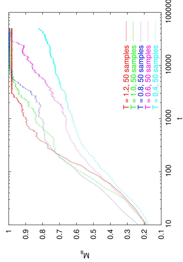
Figure 1: (Color online) Staggered magnetization as a function of time averaged over 50 samples with $L=30$ for $x=0.1$, $J/V=0.2$ and temperatures $T/J=1.2$, 1.0, 0.8, 0.6, and 0.4.

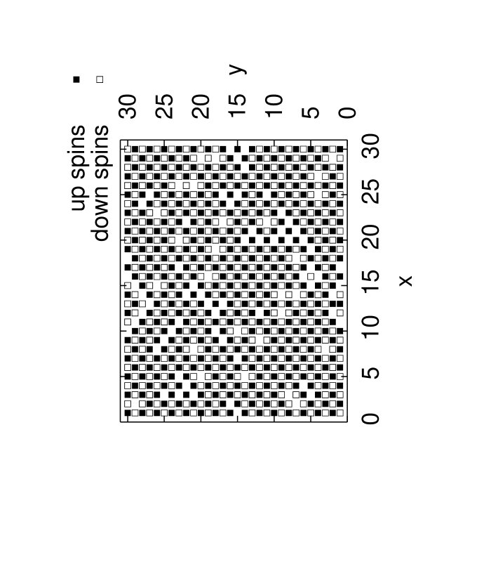
Figure 2: Illustration of the state of the system after 400 MCs in a sample with $L=30$ for $x=0.1$, $J/V=0.2$, and $T/J=0.1$. Up spins are indicated by black squares and down spins are indicated by open squares.

At larger values of $x$, there is checkerboard order in addition to Néel order, and in Fig. 3 we show the time-evolution of the checkerboard order parameter $M_{c}$ and staggered magnetization $M_{s}$ averaged over many samples for $L=30$ with $x=0.35$ at four different temperatures. Figure 4 shows the configuration reached by a low temperature sample at the same doping level after 25600 MCs. The results in the two figures appear to be consistent with the coexistence of antiferromagnetic and checkerboard order at low temperatures (the non-zero value of $M_{s}$ at $T\gtrsim 0.8$ in Fig. 3 b) is a finite size effect), and Fig. 4 appears consistent with the possibility of phase separation. We note that the time-scale for the onset of checkerboard order grows as temperature is decreased so that for $T=0.4$, the checkerboard order has not saturated in the time-window considered, even though at higher temperatures in Fig. 3 a) the value of the order parameter saturates at around $M_{c}\simeq 0.47$.

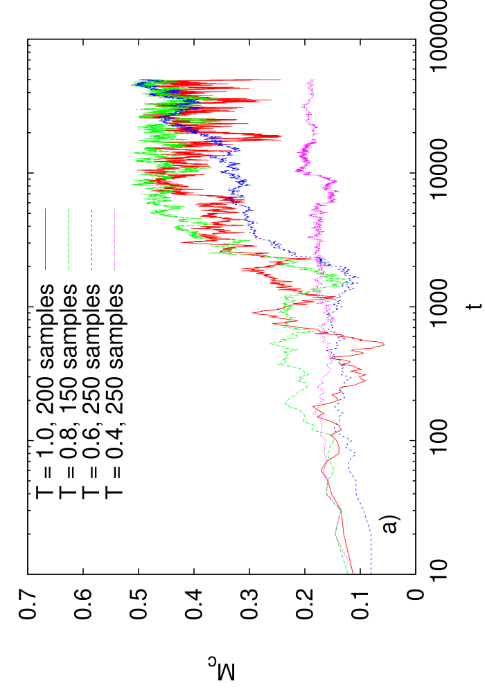
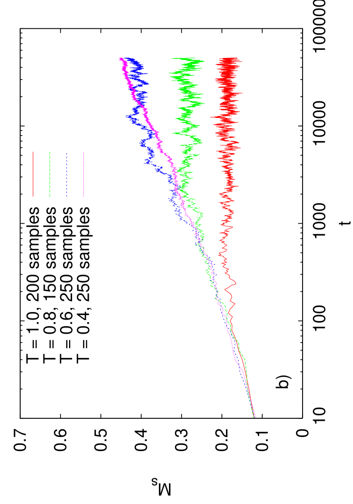
Figure 3: (Color online) a) Checkerboard order parameter and b) staggered magnetization as a function of time in Monte Carlo steps averaged at least 100 samples with $L=30$ for $x=0.35$, $T/J=0.4$, 0.6, 0.8, and 1.0, and $J/V=0.2$.

We show the phase diagram in Fig. 5 and indicate the regions in which there is Néel ordering and checkerboard ordering. The boundary of the region of Néel order, the Néel temperature, $T_{N}$, is found by calculating $M_{s}$ at $L=30$, 40, and 50 and extrapolating to where $M_{s}$ vanishes. We also find that for $x=0$, $T_{N}=2.29\pm 0.05\,J$, in agreement with the exact value of $T_{N}=2.27J$ for the two-dimensional Ising antiferromagnet. We use the same procedure with $M_{c}$ to calculate the checkerboard ordering temperature $T_{cb}$. The third temperature shown on the phase diagram is $T_{ne}$, which is the temperature below which we see stretched exponential spin relaxations, and is discussed further in Sec. III.2. From Fig. 5 it is clear that Néel order disappears as $x$ is increased towards $0.5$, and checkerboard order grows for $x\gtrsim 0.2$. For immobile holes, one expects the antiferromagnetism to disappear at the percolation threshold. The percolation threshold for bond dilution in two dimensions is $x_{c}=0.5$, Newman and for site dilution it is $x_{c}=0.41$.Stauffer ; Orbach For any one snapshot of the spin-hole configurations, there is no percolating cluster for $x>0.41$ in the thermodynamic limit, and hence we would expect that $x_{c}=0.41$. Whilst we have not investigated this question in great detail, our results are consistent with antiferromagnetism vanishing at the site dilution threshold. The slow dynamics typically occur at temperatures lower than the Néel temperature, although we note that $T_{ne}>T_{N}$ for $x=0.4$, in the region where $T_{cb}>T_{ne}>T_{N}$.

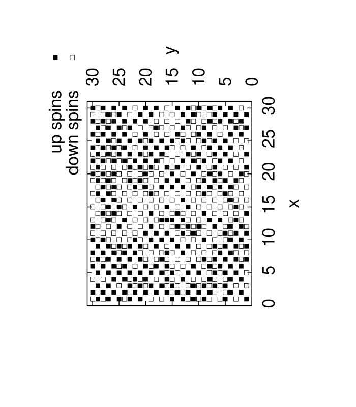
Figure 4: A configuration with checkerboard hole-ordering, and Néel ordering for $x=0.35$, $L=30$, $J/V=0.2$, and $T/J=0.1$ after 25600 MCs.

Changing the ratio of $J/V$ whilst keeping it less than 1 appears to have little effect on the Néel order, but the checkerboard transition temperature decreases rapidly as $J/V$ increases. For instance, if $J/V=0.5$ then we find that $T_{cb}/J$ is reduced to 1.3 at $x=0.5$, compared to $T_{cb}/J=3.8$ for $J/V=0.2$, as shown in Fig. 5. This appears to indicate that $T_{cb}\sim V$ at low $J/V$, whilst $T_{N}\sim J$; we have not explored the dependence of $T_{ne}$ on $J$ and $V$.

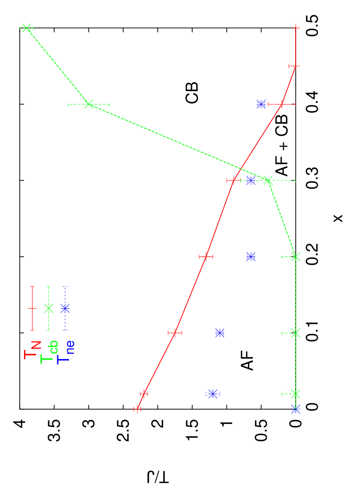
Figure 5: (Color online) Phase diagram, showing Néel temperature $T_{N}$, checkerboard ordering temperature $T_{cb}$, and onset temperature of non-exponential spin relaxation, $T_{ne}$ as a function of $x$ and $T/J$, for $J/V=0.2$. The antiferromagnetic (AF) and checkerboard (CB) regions are marked, as is the region of apparent coexistence of antiferromagnetic and checkerboard order (AF + CB).

III.2 Two-time quantities

We show the spatial and spin correlation functions as a function of $t-t_{w}$ at several different temperatures below. All data shown here for two-time correlations was taken in $L=30$ systems – the data shown is only for one thermal history, although it was checked that changing thermal history does not quantitatively change the results or fits. We note that there is some waiting time dependence of the results at low temperatures, although this is generally only for very short waiting times ($t_{w}<320$ MCs). Hence for the data we show here, we actually find that the two-time quantities depend only on time differences for the waiting times we use, so $D(t,t_{w})\simeq D(t-t_{w})$ and $C(t,t_{w})\simeq C(t-t_{w})$.

Our analysis of the data follows the following scheme. We attempt to fit

$$D(t,t_{w})=((t-t_{w})/\tau_{r})^{\alpha},$$ (7)

and

$$C(t,t_{w}) = A_{1}\,e^{-((t-t_{w})/\tau_{s})^{\beta}},$$ (8)

$$C_{local}(t,t_{w}) = A_{2}\,e^{-((t-t_{w})/\tau_{s})^{\beta}}+B,$$ (9)

where $\tau_{r}$ is the relaxation time for diffusion and $\tau_{s}$ is the relaxation time for spin correlations. Apart from very short times and very long times (where the system size becomes important for $D$, and spin correlations die out for $C$), these forms work very well (note that $A_{1}\to 1$, $A_{2}\to 0$, and $B\to 1$ at low temperatures and low doping). We use the fits to the two-time spin correlation to fit $T_{ne}$, the highest temperature at which one observes non-exponential relaxation, i.e. $\beta<1$. This temperature scale is not associated with a change in any order parameter that we measure, but allows us to determine the boundary of the region in the phase diagram where slow dynamics are observed. However, we do note that the equilibration of one-time quantities at $T<T_{ne}$ is generally much slower than for $T>T_{ne}$.

In the figures below, we only show data from $x=0.1$ unless indicated, but it is representative of the behaviour seen at other levels of doping, where we observe similar qualitative behaviour, with only quantitative differences. In Fig. 6 we show the mean square displacement as a function of time for $x=0.1$ for $J/V=0.2$.

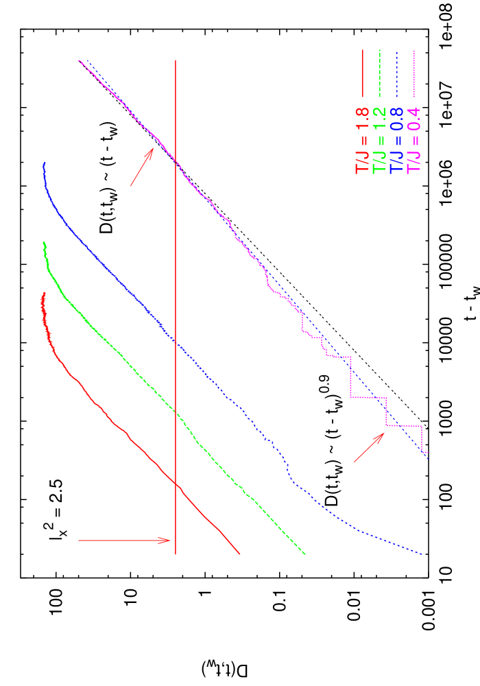
Figure 6: (Color online) Spatial correlations for $x=0.1$, $L=30$, and $J/V=0.2$ for temperatures $T/J=0.4$, 0.8, 1.2 and 1.8. Note that at the lowest temperature the slope of the curve changes, indicating anomalous diffusion. We also indicate $l_{x}^{2}=1/4x=2.5$ and the fits to $D(t,t_{w})$ at $T=0.4$ for $D(t,t_{w})<l_{x}^{2}$ and $D(t,t_{w})>l_{x}^{2}$. Note also that the saturation at long times and high temperatures is a finite size effect.

Note that at the lowest temperature in Fig. 6 there is a signature of anomalous diffusion (i.e. $\alpha<1$). This is present for mean square displacements that are less than $l_{x}^{2}=1/4x$, which is the square of the lengthscale equal to half the average distance between holes. We show a more striking example of anomalous diffusion in Fig. 7 for $x=0.02$, where the lengthscale $l_{x}^{2}$ is much larger than in Fig. 6. In general we only see anomalous diffusion at temperatures $T<T_{ne}$ and $D(t,t_{w})<l_{x}^{2}$, however the temperature where we first observe anomalous diffusion does not appear to be related to $T_{ne}$, which is when the spin auto-correlations show non-exponential relaxation. We note that anomalous diffusion has been observed in several experimental glassy systems,Weeks ; Pouliquen and can be understood as “caged” motion on short lengthscales and timescales, with usual diffusion taking over at longer timescales and lengthscales when particles have escaped from their cages. Here, the lengthscale for caging is set by the mean distance between vacancies, $l_{x}$.

Figure 7: Spatial correlations for $x=0.02$, $L=30$, and $J/V=0.2$ for temperatures $T/J=0.4$. Anomalous diffusion is clearly evident. We also indicate $l_{x}^{2}=1/4x=12.5$ and a fit to $D(t,t_{w})$ of the form $((t-t_{w})/\tau)^{0.8}$.

In Fig. 8 we show the spin correlations for $x=0.1$ and $J/V=0.2$ for several different temperatures. We note that the timescale for $C(t,t_{w})\to 0$ is of the same order as the timescale for $D(t,t_{w})\sim 1$, corresponding to the average particle having moved one lattice spacing. The argument explaining why $C(t,t_{w})\to 0$ as $t\to\infty$ in Sec. II.1.2 gives a natural explanation of why these timescales should be of the same order, and indicates the importance of the interplay between spin and diffusion dynamics, as a particle will generally be forced to flip its spin as it diffuses. For $T/J\leq 1.0$ we show both exponential and stretched exponential fits to $C(t,t_{w})$. The stretched exponentials are clearly better fits at low temperatures. We also performed calculations of $C_{local}(t,t_{w})$ for the same parameters as in Fig. 8, and these correlations are shown in Fig. 9. Whilst $C_{local}(t,t_{w})$ decays to a different limit than $C(t,t_{w})$ it also displays stretched-exponential spin relaxations at low temperatures, although at a slightly lower temperature than the $T_{ne}$ defined by $C(t,t_{w})$.

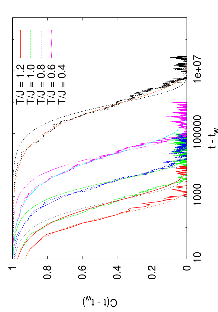
Figure 8: (Color online) Spin auto-correlations for $x=0.1$, $L=30$, and $J/V=0.2$, with $T/J=1.2$, 1.0, 0.8, 0.6, and 0.4. For $T/J\leq 1.0$ we display both exponential and stretched exponential fits to the correlations – in each of these cases, the stretched exponential is the better fit.

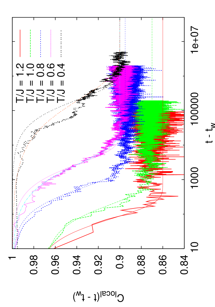
Figure 9: (Color online) Spin same-site correlations for $x=0.1$, $L=30$, and $J/V=0.2$, with $T/J=1.2$, 1.0, 0.8, 0.6, and 0.4. For $T/J\leq 0.6$ we display both exponential and stretched exponential fits to the correlations – in each of these cases, the stretched exponential is the better fit.

In Fig. 10 we show the stretched exponential $\beta$ parameter as a function of temperature for the spin auto-correlations shown in Fig. 8, which clearly indicates that the spin correlations do not decay exponentially in time at low temperatures. We also performed simulations for $x=0$, in which we found no decay of the spin correlations, indicating that the timescales observed here arise solely due to doping.

Figure 10: Stretched exponential $\beta$ parameter as a function of temperature for $x=0.1$, $L=30$, and $J/V=0.2$.

We extract values of $\tau_{r}$ and $\tau_{s}$ from fitting $D(t,t_{w})$ and $C(t,t_{w})$ as described above, and use these to define relaxation time-scales that we then fit as a function of temperature:

$$\tau_{r,s}=\tau_{0}^{r,s}+\gamma_{r,s}\exp^{\left(\frac{E_{0}^{r,s}}{T}\right)^{a_{r,s}}},$$ (10)

where $\gamma_{r,s}$, $\tau_{0}^{r,s}$, $E_{0}^{r,s}$ and $a_{r,s}$ are fitting parameters. We also tried fitting our data to a Vogel-Fulcher form, but this did not lead to good fits. We show fits of the form in Eq. (10) for $\tau_{r}$ and $\tau_{s}$ determined for $x=0.1$, $J/V=0.2$ in Figs. 11 and 12. In Table 1 we show values of $E_{0}$ and $a$ that we have extracted for $\tau_{r}$ and $\tau_{s}$ in fits of the form of Eq. (10) for different $x$. Those relating to $\tau_{r}$ are $E_{0}^{r}$ and $a_{r}$ and those relating to $\tau_{s}$ are $E_{0}^{s}$ and $a_{s}$.

$x$	$E_{0}^{r}$	$a_{r}$	$E_{0}^{s}$	$a_{s}$
0.02	10.3	0.58	10.9	0.62
0.1	8.6	0.63	8.4	0.68
0.2	7.5	0.68	7.7	0.71
0.3	6.9	0.76	7.1	0.77
0.4	6.4	0.77	6.7	0.82

Table 1: $E_{0}$ and $a$ data from fits to $\tau_{r}$ and $\tau_{s}$ made using Eq. (10)

The slowing down with temperature is similar to that seen in glass formers. However, there is a difference – in glass formers, the exponent $a$ is equal to 1 for strong glass formers (Arrhenius) and 2 for fragile glass formers (super-Arrhenius)Angell whereas the relaxation times found here consistently have $a<1$, i.e. sub-Arrhenius behaviour if one tries to fit over the entire temperature range in which there is a 6 order of magnitude change in the relaxation time. We did find however, that if we restricted the temperature range, then there is Arrhenius temperature dependence of the relaxation times at low temperatures, as is also indicated in Figs. 11 and 12. This suggests this model has strong-glass like behaviour at low temperatures.

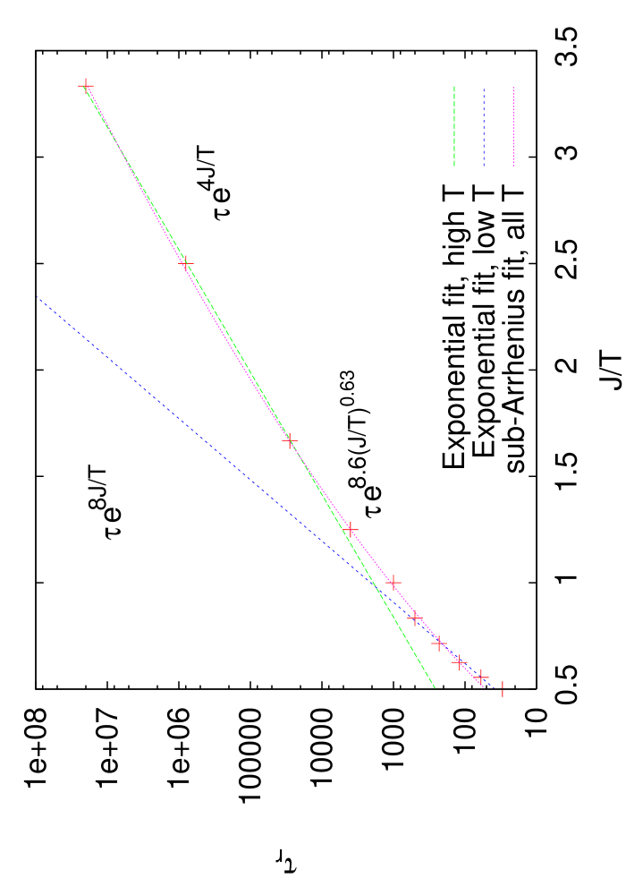
Figure 11: (Color online) Fit to diffusion relaxation times determined from spatial correlation functions as a function of temperature at $x=0.1$ and $J/V=0.2$.

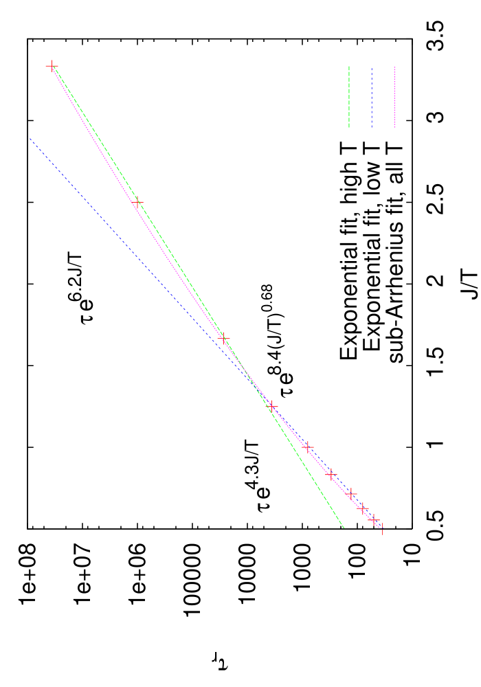
Figure 12: (Color online) Fits to spin relaxation times determined from spin correlation functions as a function of temperature at $x=0.1$, $L=30$ and $J/V=0.2$.

The diffusion relaxation time, $\tau_{r}$, and spin relaxation time $\tau_{s}$, display purely Arrhenius behaviour at low temperatures ($T<T_{ne}$), and it is possible to get a good fit to both $\tau_{r}$ and $\tau_{s}$ with an Arrhenius form at high temperatures $T>T_{ne}$, but neither fit is good over the entire temperature range, as is visible in Figs. 11 and 12.

III.3 Spin configurations

In Figs. 13 and 14 we show how changes in the configurations of spins and occupancy occur in the region where slow dynamics dominate. The doping levels used are $x=0.1$ (Fig. 13) and $x=0.3$ (Fig. 14), and both figures are for low temperatures ($T/J=0.1$). It is obvious from these plots that the dynamics is quite spatially heterogeneous at this temperature. Spin flips occur in the vicinity of holes and are facilitated by changes in occupation on adjacent sites. There are also regions in which there are no changes in spin or occupation during the time-window employed. This implies that the dynamics are a combination of vacancy motion and spin flips rather than being associated with domain wall motion. Note that the figures show where there has been a net change in occupation or a net spin flip, rather than whether this is the only change that has occurred between $t$ and $t_{w}$.

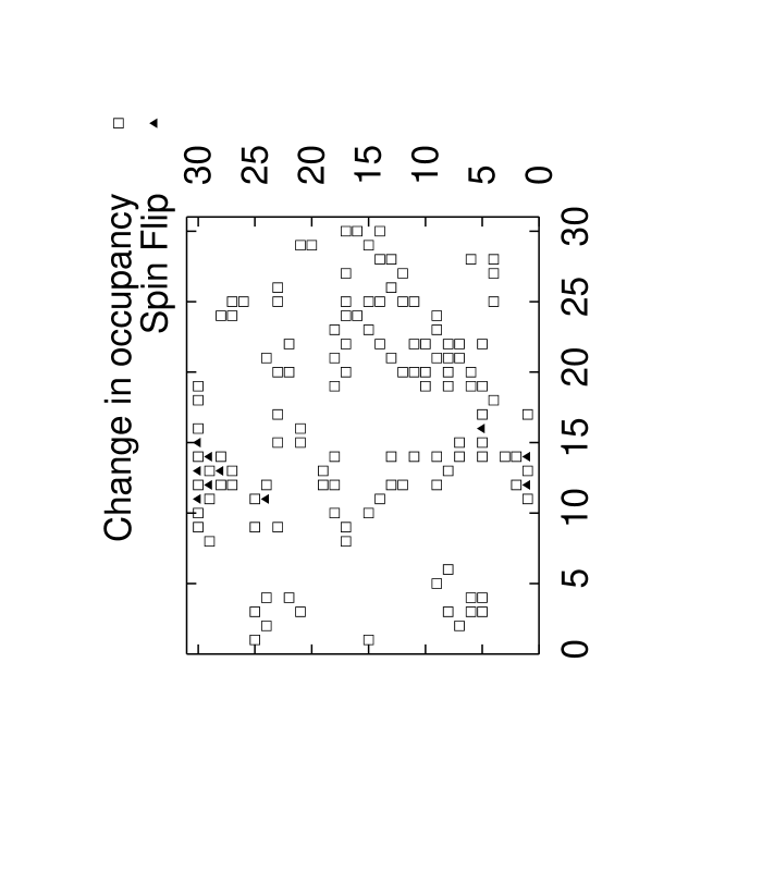
Figure 13: Illustration of the sites at which there has been a change in occupancy or a spin flip between times 400 MCs and 25600 MCs for $x=0.1$, $T/J=0.1$, $J/V=0.2$, and $L=30$.

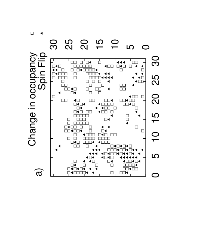
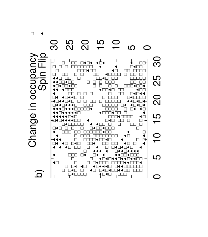
Figure 14: The two figures illustrate the sites at which there has been a change in occupancy or a spin flip between times 400 MCs and 3200 MCs for a) and between 400 MCs and 25600 MCs for b). The parameters are $x=0.3$, $T/J=0.1$, $J/V=0.2$, and $L=30$.

III.4 Distributions of correlations

In this section we show distributions of local spin correlations and displacements.Chamon To obtain these distributions, we coarse-grain the correlations that give $D(t,t_{w})$ and $C(t,t_{w})$ when averaged over all sites, over a small region about each site. More precisely, we define the coarse-grained local square displacement $D^{\rm cg}_{i}(t,t_{w})$ and coarse-grained local spin correlation $C^{\rm cg}_{i}(t,t_{w})$ as

$$D^{\rm cg}_{i}(t,t_{w}) = \frac{1}{A}\sum_{\alpha\in A_{i}(t)}\left({\mathbf{r}}_{\alpha}(t)-{\mathbf{r}}_{\alpha}(t_{w})\right)^{2},$$ (11)

$$C^{\rm cg}_{i}(t,t_{w}) = \frac{1}{A}\sum_{\alpha\in A_{i}(t)}s_{\alpha}(t)s_{\alpha}(t_{w}),$$ (12)

where $A$ is the area of the box $A_{i}(t)$, which is the box centered on site $i$, containing the set of particles $\{\alpha\}$ at time $t$. In all of the histograms shown below, we choose $A=3^{2}=9$. In Fig. 15 we show the distribution of coarse-grained local square displacements for various values of $t-t_{w}$. We find that for $t$ and $t_{w}$ with the same global mean square displacement, i.e. $D(t,t_{w})$, the distributions collapse on each other. In Fig. 16, we plot similar distributions for coarse-grained local spin auto-correlations and also see a clear scaling when the global correlation is the same. We note that for time separations such that $D(t,t_{w})$ is the same, $C(t,t_{w})$ also coincides. This scaling of distributions of local quantities with the value of the global correlation at a given time has been seen previously in investigations of other models with slow dynamics and no quenched disorder.Chamon3

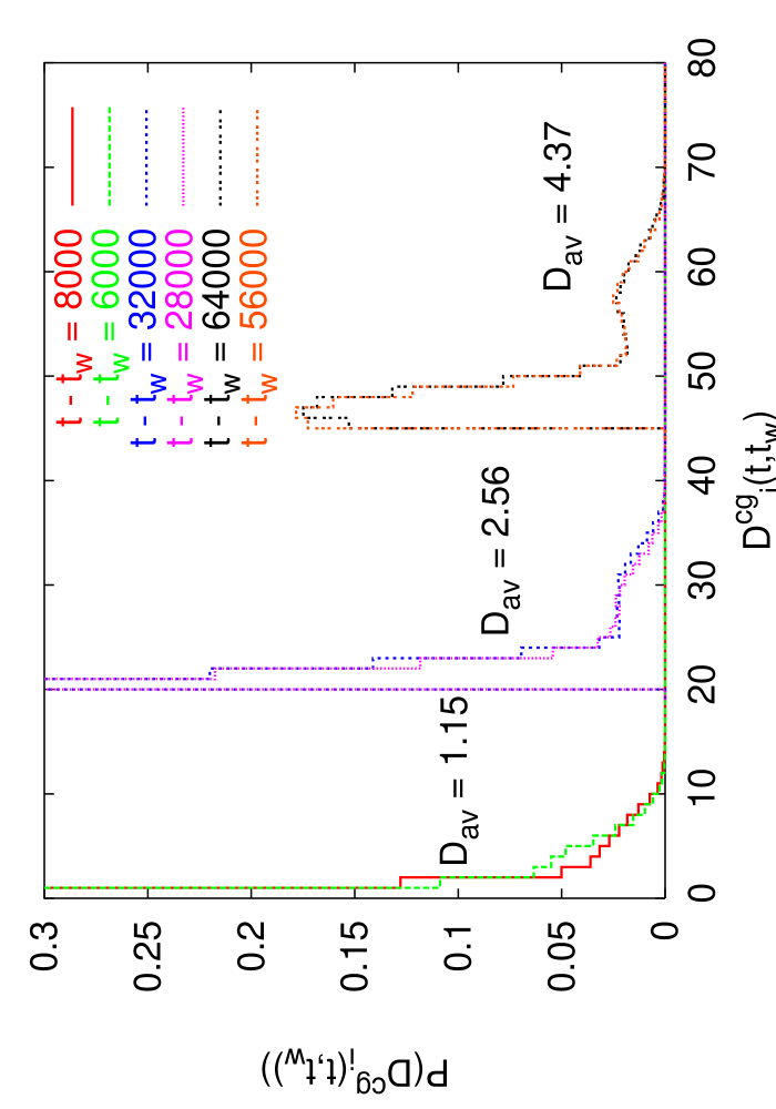
Figure 15: (Color online) Distribution of coarse-grained local square displacements for various values of $t-t_{w}$, with $x=0.1$, $T/J=0.1$, $J/V=0.2$, averaged over 20 samples of size $L=50$. We show three pairs of data, which are offset from each other along the $x$-axis, and we show the average value of the global mean square displacement $D_{\rm av}$ for each pair.

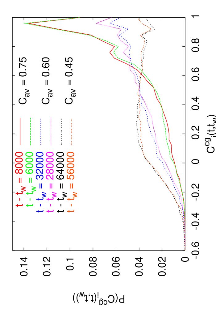
Figure 16: (Color online) Distribution of coarse-grained local spin auto-correlations for various values of $t-t_{w}$ with $x=0.1$, $T/J=0.1$, $J/V=0.2$, averaged over 20 samples of size $L=50$. We show the average value of the global spin correlation, $C_{\rm av}$ for each pair of samples.

The distributions shown in Figs. 15 and 16 appear to be stationary (i.e. depend only on $t-t_{w}$ rather than $t$ and $t_{w}$ separately). Since the distribution is stationary, it implies that its first moment is also stationary, and hence the distribution itself scales with the global correlation as follows from the arguments below. If the correlation and mean squared displacement are stationary and monotonic, then they can be written as (using the mean-squared displacement as an example)

$$D(t,t_{w})=d(t-t_{w}),$$ (13)

and for a given value of $D$ one finds the associated $t-t_{w}$:

$$D^{-1}[D]=t-t_{w}.$$ (14)

We can use similar arguments for $C(t,t_{w})$.

However, whilst the scaling of the distribution with the global correlation is trivial, the form of the distribution is not, and indicates spatially heterogeneous dynamics. In the distribution of local displacements, it is clear that as $t-t_{w}$ grows there are two populations of sites, one with fast dynamics, and another with slow dynamics. We note that the distributions displaying two populations of sites have $D(t,t_{w})\geq l_{x}^{2}$, implying that one population consists of particles still trapped in cages of size $\sim l_{x}$ and the other is those that have escaped these cages. This is reminiscent of behaviour seen recently in a two dimensional model with quenched disorderKolton and in a numerical simulation of colloidal gellation.Cates The local spin correlations do not have a clear separation into two populations of spins, but there is clearly a wide distribution of local relaxation times associated with the large spread in correlations.

IV Stokes-Einstein relation

The model studied here has several features that are reminiscent of a glass-forming liquid. At high temperatures, the mean-square displacements are linear in $t$, showing diffusive behaviour, and the relaxation times associated with this diffusion grow very quickly with decreasing temperature. These diffusive properties are what one would expect for a liquid of hard-core particles, and what we study is essentially a lattice model of this type of system. If the hard-core particles were also allowed to have a rotational degree of freedom, then again, the spin of the particles may be regarded as modelling this physics. These similarities between the model we study, and a lattice model for a liquid of hard-core particles, inspires us to ask whether well-known properties of liquids are shared by the model. In particular, it is interesting to ask whether relationships similar to the Stokes-Einstein (SE) and Debye-Stokes-Einstein (DSE) relations hold for translational and spin correlations respectively.

The SE and DSE relations describe the translation and rotational motion of a large spherical particle of radius $R$ in a hydrodynamic continuum in equilibrium at temperature $T$ with viscosity $\eta$. The SE relation predicts the dependence of the translational diffusion coefficient, ${\mathcal{D}}$, on $T$, $R$ and $\eta$:

$${\mathcal{D}}=\frac{k_{B}T}{6\pi R\eta}\;.$$ (15)

${\mathcal{D}}$ is defined from the long-time limit of the mean-square displacement, $\langle(\vec{x}(t)-\langle\vec{x}(t^{\prime})\rangle)^{2}\rangle=2d{\mathcal{D}}(t-t^{\prime})$, $d$ is the space dimension, and $k_{B}$ is Boltzmann constant. Similarly, the DSE relation predicts the dependence of the rotational correlation time, $t_{\rm rot}$ on $T$, $R$ and $\eta$:

$$t_{\rm rot}=\frac{4\pi\eta R^{3}}{3k_{B}T}\;,$$ (16)

with $t_{\rm rot}$ extracted from the decay of, say, $\frac{1}{n}\langle\vec{s}(t)\cdot\vec{s}(t^{\prime})\rangle$, where $n$ is the dimension of the orientation degree of freedom $\vec{s}$. Equations (15) and (16) imply that the product ${\mathcal{D}}t_{\rm rot}$ should not depend on $T$ and $\eta$. Even though these relations are derived for a spherical tracer, in normal liquids they are often satisfied for the translational and rotational motion of generic probes and the constituents themselves within a factor of 2.

In a supercooled fragile liquid the situation changes. While the rotational motion is consistent with Eq. (16), the diffusion of small probe molecules, Cicerone0 ; Cicerone as well as the self diffusion, Thurau ; Ediger is much faster than would be expected from the viscosity dictated by Eq. (15). The $T$ dependence of ${\mathcal{D}}$ is not given by $T/\eta$ but there is a “translational enhancement” meaning that, on average, probes translate further and further per rotational correlation time as $T_{g}$ is approached from above. For example, rotational motion in OTP is in agreement with Eq. (16) over 12 decades in viscosity while the deviation in the translational diffusion of small probe molecules of a variety of shapes, and the OTP molecules themselves, is such that the product ${\mathcal{D}}t_{\rm rot}$ increases by up to four orders of magnitude close to $T_{g}$. These results imply that molecules translate without rotating much more than DSE-SE relations would require.

The mismatch between the translational and rotational motion has been observed numerically SE-num ; Harrowell2 ; Mimo and it can be described assuming the existence of dynamic low viscosity regions, Stillinger ; Kivelson ; Cicerone a free-energy landscape based model, Dieze within the random first order transition scenario, Xia-Wolynes and kinetically facilitated spin models. KF ; Pan

Our results in Sec. III.2, where we demonstrate anomalous diffusion in Figs. 6 and 7 indicate that the SE relation breaks down at low temperatures in this model. To test whether an analogy to the DSE holds in this model, in Fig. 17 we plot the temperature dependence of the product of the translational diffusion coefficient and the characteristic time for relaxation of the spin correlation for five different values of $x$. We find that that there is strong $x$ dependence of the ratio $\tau_{s}/\tau_{r}\sim{\mathcal{D}}t_{\rm rot}$ at low temperatures: for small $x$, where there is no checkerboard ordering, $\tau_{s}/\tau_{r}$ grows at low temperatures, whereas the opposite is true for $x\gtrsim 0.2$, where checkerboard ordering is present.

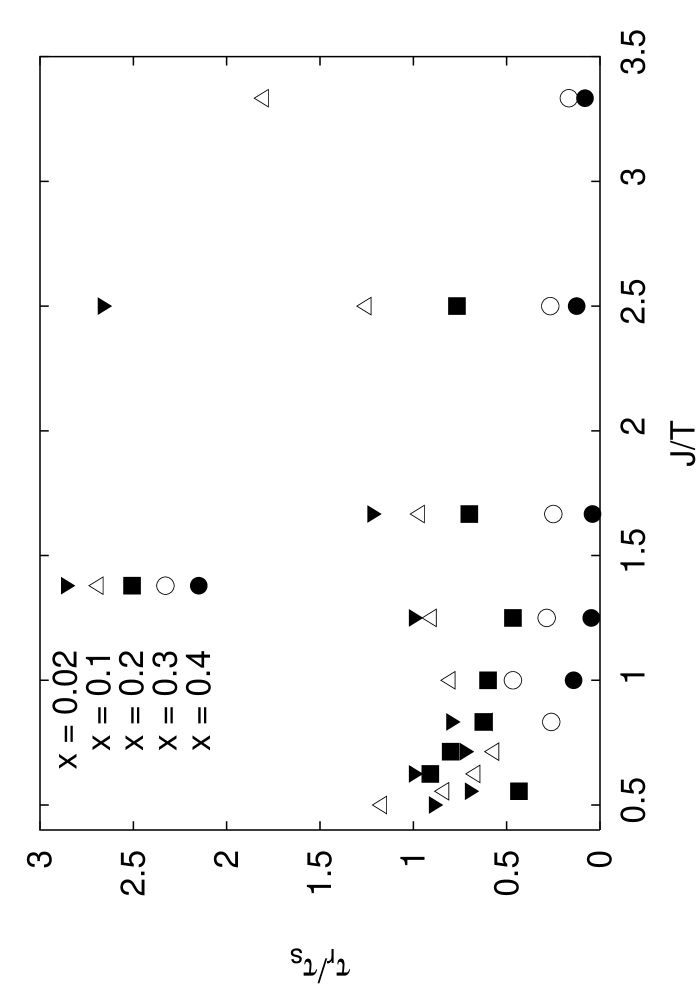
Figure 17: Ratio of diffusion and spin relaxation times as a function of temperature at $x=0.02$, 0.1, 0.2, 0.3, and 0.4, with $J/V=0.2$.

The violation of the DSE relation that we see is much smaller in magnitude than is generally seen in experiments, but this is likely to be because the model we investigate displays strong glassy behaviour, whereas experiments that study the breakdown of the SE and DSE relations are usually for fragile glass formers. The existence of an extra parameter, the doping $x$, also allows for a richer set of behaviour of ${\mathcal{D}}t_{\rm rot}$ as a function of temperature than is present in supercooled liquids.

V Discussion

We have studied a classical model for a doped antiferromagnet and found signatures of slow and heterogeneous dynamics. At low temperatures there is anomalous diffusion at lengthscales less than $l_{x}=1/2\sqrt{x}$ and stretched exponential spin relaxations. We characterize the temperature below which the slow spin relaxations occur as $T_{ne}$. For the doping levels we considered $T_{ne}$ is less than the higher of the Néel temperature $T_{N}$ and the temperature $T_{cb}$, below which checkerboard order is observed. The timescales associated with both diffusion and spin relaxation diverge at low temperatures in an Arrhenius fashion, at all doping levels considered, behaviour reminiscent of a strong glass former. Interestingly, we found that we were able to fit the temperature dependence over the entire temperature range with a sub-Arrhenius form for both $\tau_{r}$ and $\tau_{s}$. When we investigated the changes in spin configurations between two different times at several different doping levels, we found that at low temperatures, the dynamics were spatially heterogeneous, with regions of high and low mobility – we also found that spin flips were most likely to occur adjacent to regions of high mobility. This spatially heterogeneous dynamics also manifests itself in the distributions of local diffusion and spin relaxation. The distributions of local square displacements indicate that there are fast and slow populations of particles, corresponding respectively, to those which have escaped, and those which are trapped in cages with size of order $l_{x}$. The distributions of local spin correlations also indicate that there are fast and slow sites, through the wide range of relaxation times implied by the distribution. Finally, we found that when we compare $\tau_{s}$ and $\tau_{r}$ there are violations of the Debye-Stokes-Einstein relation that vary as a function of doping.

On a first glance at Eq. (1) it might appear strange that there are slow dynamics associated with this model. There is no quenched disorder, and there is no explicit frustration in the interactions as one might expect to see in a glassy model. The frustration that leads to slow dynamics appears to be hidden in the interplay of antiferromagnetic interactions and the restrictions on particle motion imposed by the level of doping. The clearest example of this is the large energy barrier to the motion of a hole to the opposite side of a plaquette. One way to relate this model to others that have been studied previously is to think about integrating out the holes, which generates a spin model with plaquette interactions, which is a generalized version of the gonihedral models that have been studied and found to have suggestions of metastable states and glassy dynamics.Gonihedral

Whilst we believe that the study of the model in this paper is of interest in itself, we also note that there is a famous class of doped two dimensional antiferromagnets, namely the high $T_{c}$ superconducting cuprates to which this work may have some connections. There are some very clear differences between our model and generic models for these materials, specifically that it is classical rather than quantum (and hence cannot show superconductivity), and also has Ising spins rather than Heisenberg spins, leading to an enhancement of long-range order in two dimensions. However, the existence of glassy spin and diffusive dynamics, in the absence of quenched disorder, along with checkerboard order, even in a classical model is very interesting. It also suggests that it might be interesting to compare quantities analogous to the SE and DSE relations for spin and charge relaxations in cuprates. We intend to investigate this model with quantum dynamics in future work. This will hopefully complement understanding gained in studying spin dynamics in doped two dimensional quantum antiferromagnets with quenched disorder.Chamon2 ; Yu

The model displays many of the features that one would expect in a lattice model for a structural glass (if one imagines the spin as corresponding to an orientation for a rod-like molecule). The temperature dependence of the relaxation times at low temperatures is consistent with that of a strong glass-former, although it is interesting that the temperature dependence over the entire temperature range can be fit with a sub-Arrhenius dependence. It maybe that dimensionality plays some role in the behaviour that we observe – it would be interesting to study this model in three dimensions to see whether similar behaviour is evident there. We note that recent experiments on two dimensional glassy films do show relaxation times that appear to have sub-Arrhenius behaviour if one fits over a temperature range that straddles $T_{g}$. Cecchetto

Another direction of research that we believe may be fruitful is, having established the existence of slow dynamics in this model to construct a field theoretic description, and to compare whether the symmetries found in the case of quenched disorder in the Edwards-Anderson model Chamon are present, and what differences exist between the two cases.

VI Acknowledgements

We thank the anonymous referee for a careful reading of the manuscript. M.P.K. acknowledges stimulating conversations with Ludovic Berthier, Horacio Castillo, David Dean, S̆imon Kos, Vadim Oganesyan, and Christos Panagopoulos. M.P.K. also acknowledges hospitality of B.U. and a Royal Society Travel Grant at the commencement of this work. L.F.C. is a member of the Institut Universitaire de France, and this research was supported in part by NSF grants DMR-0305482 and INT-0128922 (C.C.), by EPSRC grant GR/S61263/01 (M.P.K.), an NSF-CNRS collaboration, an ACI-France “Algorithmes d’optimisation et systemes desordonnes quantiques”, and the STIPCO European Community Network (L.F.C.).

References

- (1) J. G. Bednorz and K. A. Muller, Z. Phys. B 64, 189 (1986).
- (2) P. W. Anderson, Science 235, 1196 (1987).
- (3) A. Aharony, R. J. Birgeneau, A. Coniglio, M. A. Kastner, and H. E. Stanley, Phys. Rev. Lett. 60, 1330 (1988).
- (4) F. C. Chou, N. R. Belk, M. A. Kastner, R. J. Birgeneau, and A. Aharony, Phys. Rev. Lett. 75, 2204 (1995); M. A. Kastner, R. J. Birgeneau, G. Shirane, and Y. Endoh, Rev. Mod. Phys. 70, 897 (1998); S. Wakimoto, S. Ueki, Y. Endoh, and K. Yamada, Phys. Rev. B 62, 3547 (2000); A. N. Lavrov, Y. Ando, S. Komiya, and I. Tsukada, Phys. Rev. Lett. 87, 017007 (2001).
- (5) C. Panagopoulos, A. P. Petrovic, A. D. Hillier, J. L. Tallon, C. A. Scott, and B. D. Rainford, Phys. Rev. B 69, 144510 (2004).
- (6) C. Panogopoulos and V. Dobrosavljević, cond-mat/0410111.
- (7) J. E. Hoffman, E. W. Hudson, K. M. Lang, V. Madhavan, H. Eisaki, S. Uchida, and J. C. Davis, Science 295, 466 (2002); M. Vershinin, S. Misra, S. Ono, and Y. Abe, Science 303, 1995 (2004); K. McElroy, D.-H. Lee, J. E. Hoffman, K. M. Lang, J. Lee, E. W. Hudson, H. Eisaki, S. Uchida, and J. C. Davis, cond-mat/0406491.
- (8) T. Hanaguri, C. Lupien, Y. Kohsaka, D.-H. Lee, M. Azuma, M. Takano, H. Takagi, and J. C. Davis, Nature 430, 1001 (2004).
- (9) G. H. Fredrickson and H. C. Andersen, Phys. Rev. Lett. 53, 1244 (1984).
- (10) J. Jäckle and S. Eisinger, Z. Phys. B 84, 115 (1991).
- (11) J. Kurchan, L. Peliti, and M. Selitto, Europhys. Lett. 39, 365 (1997); M. Selitto, Eur. Phys. J. B 4, 135 (1998).
- (12) M. A. Muoz, A. Gabrielli, H. Inaoka, and L. Pietronero, Phys. Rev. E 57, 4354 (1998).
- (13) P. Sollich and M. R. Evans, Phys. Rev. Lett. 83, 3238 (1999).
- (14) J. P. Garrahan and D. Chandler, Phys. Rev. Lett. 89, 035704 (2002); Proc. Nat. Acad. Sci. 100, 9710 (2003).
- (15) F. Ritort and P. Sollich, Adv. Phys. 52, 219 (2003).
- (16) C. Toninelli, G. Biroli, and D. S. Fisher, Phys. Rev. Lett. 92, 185504 (2004); C. Toninelli and G. Biroli, J. Stat. Phys. 117, 27 (2004); C. Toninelli, G. Biroli, and D. S. Fisher, cond-mat/0410647.
- (17) L. Berthier and J. P. Garrahan, J. Phys. Chem. B 109, 3578 (2005).
- (18) L. Berthier, Proc. SPIE Int. Soc. Opt. Eng. 177, 5469 (2004).
- (19) D. N. Perera and P. Harrowell, J. Non-Cryst. Sol. 235, 314 (1998).
- (20) H. Sillescu, J. Non. Cryst. Solids 243, 81 (1999).
- (21) M. D. Ediger, Annu. Rev. Phys. Chem. 51, 99 (2000).
- (22) A. Coniglio, Proc. of the International School on the Physics of Complex Systems, Varenna (1996); M. Nicodemi and A. Coniglio, J. Phys. A. Lett. 30, L 187 (1996); J. Arenzon, M. Nicodemi, M. Sellitto, J. de Phys. I (France) 6, 1143 (1996); A. Fierro, G. Franzese, A. de Candia, and A. Coniglio, Phys. Rev. E 59, 60 (1999); A. Coniglio, A. de Candia, A. Fierro, and M. Nicodemi, J. Phys. C 11, A167 (1999); F. Ricci-Tersenghi, D. A. Stariolo, J. J. Arenzon, Phys. Rev. Lett. 84, 4473 (2000); A. Fierro, A. de Candia, and A. Coniglio, Phys. Rev. E 62, 7715 (2000); A. Fierro, A. de Candia, and A. Coniglio, J. Phys. Cond. Mat. 14, 1549 (2002); A. de Candia, A. Fierro, and A. Coniglio, Fractals 11, 99 Suppl. (2003); M. H. Vainstein, D. A. Stariolo, J. J. Arenzon, J. Phys. A 36, 10907 (2003).
- (23) M. Nicodemi and A. Coniglio, Phys. Rev. E 57, R39 (1998).
- (24) W. Ertel, K. Froböse, and J. Jäckle, J. Chem. Phys. 88, 5027 (1988); J. Jäckle, J. Phys. Cond. Mat. 14, 1423 (2002).
- (25) C. Chamon, P. Charbonneau, L. F. Cugliandolo, D. R. Reichmann, and M. Selitto, J. Chem. Phys. 121, 10120 (2004).
- (26) S. A. Kivelson, V. J. Emery, and H. Q. Lin, Phys. Rev. B 42, 6523 (1990).
- (27) E. W. Carlson, S. A. Kivelson, Z. Nussinov, and V. J. Emery, Phys. Rev. B 57, 14704 (1998).
- (28) Whilst we set particle moves and spin flips to have equal weight, changing the weight of one or the other does not appear to affect our results qualitatively.
- (29) An alternative dynamics that one might consider would allow the particle to attempt to move to any of its neighbours, where attempts to move to occupied sites are unsuccessful, but contribute to the number of Monte Carlo steps. We checked that this gives the same qualitative features as our results, except with longer time-scales. For , we find the same value of (defined in Sec. III.2) as with the dynamics we use in the rest of the paper.
- (30) S. A. Trugman, Phys. Rev. B 37, 1597 (1988).
- (31) L. F. Cugliandolo and J. Kurchan, Phys. Rev. Lett. 71, 173 (1993).
- (32) J.-P. Bouchaud, L. F. Cugliandolo, J. Kurchan, and M. Mezard, in Spin-Glasses and Random Fields, ed. A. P. Young (World Scientific, 1998), cond-mat/9702070; L. F. Cugliandolo, Lecture notes in Slow Relaxation and non equilibrium dynamics in condensed matter, Les Houches Session 77 July 2002, eds. J.-L. Barrat, J. Dalibard, J. Kurchan, M. V. Feigel’man, cond-mat/0210312.
- (33) Note that in the time window considered, and saturate at high temperature, but do not for lower temperatures, which is why we keep the time depdendence in the staggered magnetization.
- (34) M. E. J. Newman, and R. M. Ziff, Phys. Rev. Lett. 85, 4104 (2000).
- (35) D. Stauffer and A. Aharony, Introduction to Percolation Theory, 2nd ed. (Taylor and Francis, London, 1994).
- (36) T. Nakayama, K. Yakubo, and R. L. Orbach, Rev. Mod. Phys. 66, 381 (1994).
- (37) E. R. Weeks, J. C. Crocker, A. C. Levitt, A. Schofield, and D. A. Weitz, Science 287, 627 (2000); E. Courtland and E. R. Weeks, J. Phys. Cond. Mat. 15, S359 (2003).
- (38) O. Pouliquen, M. Belzons, and M. Nicolas, Phys. Rev. Lett. 91, 014301 (2003).
- (39) L. M. Martinez and C. A. Angell, Nature 410, 663 (2001); C. A. Angell, J. Phys. Condens. Mat. 12, 6463 (2000).
- (40) C. Chamon, M. P. Kennett, H. E. Castillo, and L. F. Cugliandolo, Phys. Rev. Lett. 89 217201 (2002); H. E. Castillo, C. Chamon, L. F. Cugliandolo, and M. P. Kennett, Phys. Rev. Lett. 88, 237201 (2002); H. E. Castillo, C. Chamon, L. F. Cugliandolo, J. L. Iguain, and M. P. Kennett, Phys. Rev. B 68, 134442 (2003).
- (41) A. B. Kolton, D. R. Grempel, and D. Domínguez, cond-mat/0407734; D. R. Grempel, Europhys. Lett. 66, 854 (2004).
- (42) A. M. Puertas, M. Fuchs, and M. E. Cates, cond-mat/0409740.
- (43) M. T. Cicerone, F. R. Clackburn, and M. D. Ediger, Macromolecules 28, 8224 (1995).
- (44) M. T. Cicerone and M. D. Ediger, J. Chem. Phys. 104, 7210 (1996).
- (45) C. T. Thurau and M. D. Ediger, J. Chem. Phys. 116, 9089 (2002); C. T. Thurau and M. D. Ediger, J. Chem. Phys, 118, 1996 (2003).
- (46) S. F. Swallen, P. A. Bonvallet, R. J. McMahon, and M. D. Ediger, Phys. Rev. Lett. 90, 015901 (2003).
- (47) J.-L. Barrat, J.-N. Roux, and J.-P. Hansen, Chem. Phys. 149, 197 (1990); D. Thirumalai and R. D. Mountain, Phys. Rev. E 47, 479 (1993); D. N. Perera and P. Harrowell, Phys. Rev. Lett. 81, 120 (1998); S. C. Glotzer, V. N. Novikov, and T. B. Shroder, J. Chem. Phys. 112, 500 (2000).
- (48) D. N. Perera and P. Harrowell, Phys. Rev. Lett. 80 4446 (1998); ibid 81, 120 (1998).
- (49) G. Tarjus and D. Kivelson, J. Chem. Phys. 103, 1995 (1995); D. Kivelson, S. A. Kivelson, X. L. Zhao, Z. Nussinov, and G. Tarjus, Physica A 219, 27 (1995).
- (50) F. H. Stillinger and J. A. Hodgdon, Phys. Rev. E 50, 2064 (1994).
- (51) G. Diezemann, J. Chem. Phys. 107, 10112 (1997); G. Diezemann, H. Sillescu, G. Hinze and R. Böhmer, Phys. Rev. E 57, 4398 (1998).
- (52) X. Xia and P. G. Wolynes, Proc. Nat. Acad. Sci. 97, 2990 (2000).
- (53) Y. J. Jung, J. P. Garrahan, and D. Chandler, Phys. Rev. E 69, 061205 (2004).
- (54) A. C. Pan, J. P. Garrahan, and D. Chandler, cond-mat/0410525.
- (55) G. K. Bathas, E. Floratos, G. K. Savvidy, and K. G. Savvidy, Mod. Phys. Lett. A 10, 2695 (1995); A. Lipowski and D. Johnston, J. Phys. A 33, 4451 (2000); P. Dimopoulos, D. Espriu, E. Jané, and A. Prats, Phys. Rev. E 66, 056112 (2002).
- (56) E. Mucciolo, A. H. Castro-Neto, and C. Chamon, Phys. Rev. B 69, 214424 (2004).
- (57) R. Yu, T. Roscilde, and S. Haas, cond-mat/0410041.
- (58) E. Cecchetto, D. Moroni, and B. Jérôme, cond-mat/0402656.