Sensitivity to initial conditions in coherent noise models

Abstract

Sensitivity to initial conditions in the coherent noise model of biological evolution, introduced by Newman, is studied by making use of damage spreading technique. A power-law behavior has been observed, the associated exponent $\alpha$ and the dynamical exponent $z$ are calculated. Using these values a clear data collapse has been obtained.

PACS Number(s): 89.75.Da, 05.90.+m, 91.30.-f

It is clear that there is an increasing interest in extended dynamical systems exhibiting avalanches of activity, whose size distribution is scale-free. Some examples of such systems can be enumerated as earthquakes earth , rice piles sand , extinction in biology ext , evolving complex networks nets , etc. However, there is no unique and unified theory for such systems. One of the possible candidates is the notion of self-organize criticality (SOC) soc . In SOC models, the whole system is under the influence of a small driving force that acts locally and these systems evolve towards a critical stationary state having no characteristic spatio-temporal scales. On the other hand, it is known from literature newman1 that another kind of simple and robust mechanism is available in order for producing scale-free behavior. This mechanism is based on the notion of external stress coherently imposed on all agents of the system. Since the model does not contain any direct interaction among agents, it does not exhibit criticality. Nevertheless, it yields a power-law distribution of event size. These so-called coherent noise models have been firstly introduced to describe large-scale events in evolution, but then they were used as a model of earthquakes newman2 and its aftershock properties wilkeD as well as aging phenomenon in the model ugur have been analysed.

The coherent noise models can be defined as follows: Firstly we consider a system, which has $N$ agents. Each agent $i$ has a threshold $x_{i}$ against external stress $\eta$. The threshold levels are chosen randomly from some probability distribution $p_{thresh}(x)$. The external stress is also drawn randomly from another distribution $p_{stress}(\eta)$. An agent is eliminated if it is subjected to the stress $\eta$ exceeding the threshold for this agent. Algorithmically, dynamics of the model can be given by three steps: (i) at each time step, generate a random stress $\eta$ from $p_{stress}(\eta)$, eliminate all agents with $x_{i}\leq\eta$ and replace them by new agents with new thresholds taken from $p_{thresh}(x)$, (ii) select a small fraction $f$ of the $N$ agents at random and assign them new thresholds, (iii) go back to (i) for the next time step. It is worth mentioning that step (ii) corresponds to the probability for the $f$ fraction of the whole agents of undergoing spontaneous transition, which is a step necessary for preventing the model from grinding to a halt wilkeD .

In the present work, we focus on the sensitivity to the initial conditions of the coherent noise models using damage spreading technique. This technique can be thought as a method which is borrowed from dynamical systems theory in the following sense: If we consider two copies of the same one-dimensional dynamical system starting from slightly different initial conditions and follow their time evolution, we can define the sensitivity function

$$\xi(t)\equiv\lim_{\Delta x(0)\rightarrow 0}\frac{\Delta x(t)}{\Delta x(0)}=e^{\lambda t}$$ (1)

to quantify the effect of initial conditions. Here, $\Delta x(0)$ and $\Delta x(t)$ are the distances between two copies at $t=0$ and $t$ respectively, and $\lambda$ is the Lyapunov exponent. If $\lambda>0$ ($\lambda<0$), the system is said to be strongly sensitive (strongly insensitive) to the initial conditions. For the marginal case, where $\lambda=0$, the form of the sensitivity function could be a whole class of functions. For the low-dimensional discrete dynamical systems, this form is found to be a power-law

$$\xi(t)\sim t^{\alpha}\;\;\;.$$ (2)

The $\alpha>0$ and $\alpha<0$ cases correspond to weakly sensitive and weakly insensitive to the initial conditions maps . For the high-dimensional dynamical systems, like the Bak-Sneppen model or like the one that we discuss in this work, the same analysis could be performed using the Hamming distance instead of the sensitivity function. As in the case of low-dimensional systems, one can classify the sensitivity by looking at the behavior of the Hamming distance

$$D(t)=\frac{1}{N}\sum_{i=1}^{N}\left|x_{i}^{(1)}(t)-x_{i}^{(2)}(t)\right|\;\;,$$ (3)

where $x_{i}^{(1)}$ and $x_{i}^{(2)}$ are two slightly different copies of the system under consideration. In this way, up to now, various variants of the Bak-Sneppen model have been analysed and related exponents are calculated tamarit ; vega1 ; vega2 ; ugurlyra1 ; ugurlyra2 . Our aim here is to make the same analysis for the coherent noise models to numerically obtain the dynamical exponents of the model.

To proceed further let us define the procedure. We start the simulations from a uniform threshold distribution, which means that the system starts from an initial event of infinite size that spans the whole system. This is considered to be the first copy of the system (namely, $x_{i}^{(1)}$). In all simulations, we use the exponential distribution for the external stress

$$p_{stress}(\eta)=a^{-1}\exp\left(-\frac{\eta}{a}\right)\;\;\;\;(a>0)\;\;,$$ (4)

and the uniform distribution $p_{thresh}(x)$ $(0\leq x\leq 1)$ for the threshold level. The second copy (namely, $x_{i}^{(2)}$) is generated by exchanging the values of two randomly chosen sites. Then the dynamics of the model, as explained above, is applied for both copies of the system using always the same set of random numbers to update them. To investigate the properties of sensitivity to initial conditions of the model, we follow the temporal evolution of the Hamming distance given in Eq.(3). In all cases, we use a large number of realizations to reduce the fluctuations and the given results, namely $\left<D(t)\right>$, are the ensemble averages over these realizations. From Fig. 1 it is easily seen that the damage spreads as a power-law, indicating a weak sensitivity to initial conditions. Obviously, the power law growth $\left<D(t)\right>\sim t^{\alpha}$ with $\alpha=0.95\pm 0.04$ is followed by a plateau with a constant value, starting at a certain time depending on the system size. This saturation is due to the fact that by this measure one cannot identify that both copies have converged to the same random sequence.

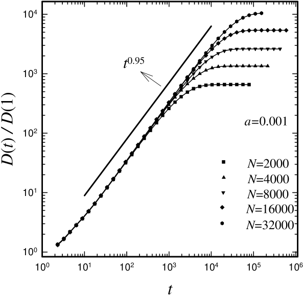
Figure 1: Time evolution of the normalized Hamming distance for five different system sizes. For the largest one ($N=32000$) the exponent of the power-law growth is estimated as $\alpha=0.95\pm 0.04$ The number of realizations used for averaging is 200 for $N=32000$ and 400 otherwise. For a better visualization logaritmic binning is employed to all data sets.

The second important exponent, called as the dynamical exponent $z$, comes from the scaling of $\tau(N)$, which is defined to be the value of $t$ where the power-law increasing part crosses over onto the saturation regime. More precisely, $\tau$ is the value of $t$ at the intersection point of two straight lines, one of which comes from the power-law curve and the other from the constant plateau. Then, the scaling $\tau(N)\sim N^{z}$ defines the dynamical exponent $z$, which is obtained from Fig. 2 as $z=0.96\pm 0.02$.

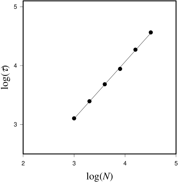
Figure 2: Double log plot of $\tau$ versus $N$ for each curve given in Fig. 1. From this scaling we estimate the dynamical exponent as $z=0.96\pm 0.02$.

As a final step, we analyse the finite size scaling behavior of the model. To accomplish this task, we define the normalized Hamming distance as

$$D(N,t)=\frac{\left<D(t)\right>}{\left<D(1)\right>}$$ (5)

and numerically verify that it obeys the scaling ansatz

$$D(N,t)=N^{\beta}F\left(\frac{t}{N^{\gamma}}\right)\;\;,$$ (6)

with $\beta=0.91$, which comes from $\beta=\gamma\alpha$ and $\gamma=z$. A clear data collapse can easily be seen in Fig. 3. It is worth noting that the results presented here do not depend on the choice of the numerical value of the model parameter $a$ and/or the fraction $f$. In our simulations we use $a=0.001$ and different $f$ values for each system size in order to assure only one agent is eliminated in step (ii) to reduce the computational time.

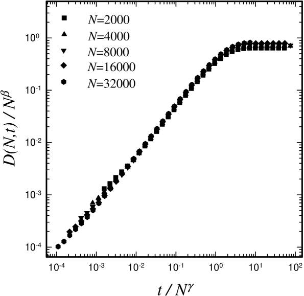
Figure 3: Data collapse of the finite size scaling given in Eq.(6) for the same system sizes used in Fig. 1 and Fig. 2.

Summing up, we have studied the sensitivity to initial condition properties of the coherent noise models using damage spreading technique. We found that the model exhibits weak sensitivity to initial conditions, a property which is common for other high-dimensional dynamical systems like Bak-Sneppen model and its variants as well as one- and two-dimensional discrete systems like logistic map families. The numerically obtained values of the power-law exponent $\alpha$ and the dynamical exponent $z$ are appeared to be different from those of the Bak-Sneppen model, which signals out the discrepancy between the universality classes of these models.

References

- (1) J.F. Pacheco, C.H. Scholz and L.R. Sykes, Nature 255, 71 (1997).
- (2) V. Frette et al., Nature 379, 49 (1996).
- (3) R.V. Sole and J. Bascompte, Proc. Roy. Soc. London B 263, 161 (1997).
- (4) R. Albert and A.L. Barabasi, Rev. Mod. Phys. 74, 47 (2002).
- (5) P. Bak, C. Tang and K. Wiesenfeld, Phys. Rev. Lett. 59, 381 (1987).
- (6) M.E.J. Newman, Proc. R. Soc. London B 263, 1605(1996).
- (7) M.E.J. Newman and K. Sneppen, Phys. Rev. E 54, 6226 (1996); K. Sneppen and M.E.J. Newman, Physica D 110, 209 (1997).
- (8) C. Wilke, S. Altmeyer, and T. Martinetz, Physica D 120, 401 (1998).
- (9) U. Tirnakli and S. Abe, Phys. Rev. E 70, (1 November 2004), in press.
- (10) C. Tsallis, A.R. Plastino, W.-M. Zheng, Chaos, Solitons and Fractals 8 (1997) 885; U. Tirnakli, C. Tsallis and M.L. Lyra, Eur. Phys. J. B 11, 309 (1999); U. Tirnakli, C. Tsallis and M.L. Lyra, Phys. Rev. E 65, 036207 (2002); U. Tirnakli, Phys. Rev. E 66, 066212 (2002); F. Baldovin, A. Robledo, Phys. Rev. E 66, 045104 (2002); F. Baldovin, A. Robledo, Europhys. Lett. 60, 066212 (2002).
- (11) F.A. Tamarit, S.A. Cannas and C. Tsallis, Eur. Phys. J. B 1, 545 (1998).
- (12) R. Cafiero, A. Valleriani and J.L. Vega, Eur. Phys. J. B 7, 505 (1999).
- (13) A. Valleriani and J.L. Vega, J. Phys. A: Math. Gen. 32, 105 (1999).
- (14) U. Tirnakli and M.L. Lyra, Int. J. Mod. Phys. C 14, 805 (2003).
- (15) U. Tirnakli and M.L. Lyra, Physica A 342, 151 (2004).