BCS-BEC crossover with a finite-range interaction

Abstract

We study the crossover from BEC to BCS pairing for dilute systems but with a realistic finite-range interaction. We exhibit the changes in the excitation spectrum that provide a clean qualitative distinction between the two limits. We also study how the dilute system converges to the results from a zero-range pseudo-potential derived by Leggett.

I Introduction

Ultracold atomic gases provide an experimental playground for testing pairing phenomena, due to the ability to control the inter-atomic interactions via a magnetically-tuned Feshbach resonance ref:TVS93 . Over the past year, tremendous progress has been made in realizing the crossover from the Bose-Einstein condensation (BEC) of diatomic molecules to the Bardeen-Cooper-Schrieffer (BCS) limit of weakly-bound Cooper pairs in ultracold gases of fermionic atoms fermi_exp ; exp_04 . But there is much debate over where the crossover between the BCS and BEC regimes occurs, following recent experimental studies on fermionic condensates exp_04 . Therefore, it is timely to perform a thorough theoretical investigation of what the signature of the crossover is and how it might be observed experimentally, using a realistic potential with a finite range.

Much of the theoretical work on systems of two types of fermions interacting via an adjustable, attractive potential have focussed on interactions that are governed by a single parameter, namely the s-wave scattering length $a_{0}$ ref:leg80 ; ref:ran . Such a description is valid provided we have $|a_{0}|\gg\langle r\rangle$ and $k_{F}\langle r\rangle\ll 1$, where $\langle r\rangle$ is the width of the potential and $k_{F}$ is the Fermi momentum of the non-interacting system, so that the only independent dimensionless variable in the problem is $a_{0}k_{F}$. Thus, it is only applicable to dilute systems like the ultracold atomic gases, not the high density situation found in conventional superconductors ref:schr . The potential supports a 2-body bound state for $(a_{0}k_{F})^{-1}~{}>~{}0$, but this molecular state passes through zero energy and vanishes into the continuum at $(a_{0}k_{F})^{-1}=0$, the position of the Feshbach resonance. As such, the BCS and BEC limits correspond to $(a_{0}k_{F})^{-1}~{}\rightarrow~{}-\infty$ and $(a_{0}k_{F})^{-1}\rightarrow+\infty$, respectively.

The distinction between the BEC and BCS regimes can be made sharper ref:leg80 : the qualitative boundary between the BCS and BEC ground states occurs when the chemical potential $\mu$ reaches $0$, marking the disappearance of a Fermi surface, and this coincides with the appearance of a bound state at $(a_{0}k_{F})^{-1}=0$ only when the density is zero. At the point where there is no longer a defined Fermi surface, there are qualitative changes in the quasi-particle excitation spectrum: the momentum corresponding to the minimum in the excitation spectrum shifts from finite momentum in the BCS limit to zero momentum in the BEC limit. At the same point, the value of the excitation gap goes from $\Delta$ in the BCS limit to $\sqrt{\mu^{2}+\Delta^{2}}$ in the BEC limit, where $\Delta$ is the gap parameter. We shall use these changes in the excitation spectrum as the “definition” of the crossover point.

There have also been studies of the BCS-BEC crossover using Coulomb potentials in the context of excitons ref:CN82 . Here, the interaction is kept fixed and the density varied to achieve a smooth transition from the high density BCS limit to the dilute BEC limit. Note that it is not possible to obtain a density-driven crossover using an interaction that is only characterized by the scattering length, since this picture breaks down at high densities.

In this paper, we shall study the BCS-BEC crossover at zero temperature using a realistic Gaussian potential and compare with results from single-parameter potentials. We use a mean-field variational wave function to describe the crossover, which is expected to give an accurate description of the low temperature behavior, though not, of course, the finite temperature transition.

The paper is organized as follows: We describe the model and variational scheme in Sec. II. We discuss the characteristics of the wave functions and excitation spectra in Sec. III. In Sec. IV we compare our results with Leggett’s zero-range pseudo-potential result which is usually used to describe the mean-field limit for dilute Fermi systems. We conclude in Sec. V.

II Formalism

We determine the ground-state wave function $|\Phi\rangle$ using conventional mean-field methods, briefly reviewed here. We consider the Hamiltonian

$$\hat{H}=\sum_{\mathbf{k},i}\epsilon_{\mathbf{k}}\ a^{{\dagger}}_{\mathbf{k}i}a_{\mathbf{k}i}+\ \sum_{\mathbf{k,p,q}}V_{\mathbf{q}}\ a^{{\dagger}}_{\mathbf{k}\uparrow}a^{{\dagger}}_{\mathbf{p}\downarrow}a_{\mathbf{p}-\mathbf{q}\downarrow}a_{\mathbf{k}+\mathbf{q}\uparrow}\>,$$ (1)

where $\mathbf{k}$ and $i$ denote momentum variables and spin states $\{\uparrow,\downarrow\}$, respectively, and $\epsilon_{\mathbf{k}}=\hbar^{2}\mathbf{k}^{2}/2m$. Since experiments on atomic gases are carried out at low energies, we will restrict ourselves to the simple case of an s-wave pairing interaction.

We calculate the ground state by minimizing the free energy

$$\mathbf{F}\ =\ \langle\Phi|\hat{H}-\mu\hat{N}|\Phi\rangle\>,$$ (2)

where $\hat{N}=\sum_{\mathbf{k},i}a^{{\dagger}}_{\mathbf{k}i}a_{\mathbf{k}i}$ is the total number operator and $\mu$ is the chemical potential. The standard BCS variational wave function is given by

$$|\Phi\rangle\ =\ \mathcal{N}\ \exp\left(\sum_{\mathbf{k}}\ \frac{v_{\mathbf{k}}}{u_{\mathbf{k}}}\ a^{{\dagger}}_{\mathbf{k}\uparrow}a^{{\dagger}}_{-\mathbf{k}\downarrow}\right)\ |0\rangle\>,$$ (3)

and it smoothly interpolates from the BCS to BEC limits, giving an accurate description of the crossover. Here, the BCS parameters $u_{\mathbf{k}}$, $v_{\mathbf{k}}$ only depend on $k\equiv|\mathbf{k}|$ in the s-wave approximation, and $\mathcal{N}=\prod_{\mathbf{k}}u_{\mathbf{k}}$ is the normalization constant, such that $\langle\Phi|\Phi\rangle=1$. With this ansatz, the free energy becomes

$$\mathbf{F}\ =\ 2\ \sum_{\mathbf{k}}\ (\epsilon_{\mathbf{k}}-\mu)\ \rho_{\mathbf{k}}\ +\ \sum_{\mathbf{k,p}}\ V_{\mathbf{p}-\mathbf{k}}\ \kappa^{*}_{\mathbf{k}}\kappa_{\mathbf{p}}\>,$$ (4)

where the normal and anomalous densities are

$$\rho_{\mathbf{k}}\ =\ \langle\Phi|{\mathbf{a}}^{\dagger}_{\mathbf{k}\uparrow}{\mathbf{a}}_{\mathbf{k}\uparrow}|\Phi\rangle\ =\ |v_{\mathbf{k}}|^{2}\>,$$ (5)

and

$$\kappa_{\mathbf{k}}\ =\ \langle\Phi|{\mathbf{a}}_{-\mathbf{k}\downarrow}{\mathbf{a}}_{\mathbf{k}\uparrow}|\Phi\rangle\ =\ v_{\mathbf{k}}^{*}u_{\mathbf{k}}\>,$$ (6)

respectively, subject to the normalization condition,

$$|u_{\mathbf{k}}|^{2}\ +\ |v_{\mathbf{k}}|^{2}\ =\ 1\>.$$ (7)

Without loss of generality we can choose $u_{\mathbf{k}}$ and $v_{\mathbf{k}}$ to be real.

After minimization, the resulting equations we have to solve are

$$\Delta_{\mathbf{k}}\ =\ -\ \sum_{\mathbf{p}}\ V_{\mathbf{k}-\mathbf{p}}\ \frac{\Delta_{\mathbf{p}}}{E_{\mathbf{p}}}\>,$$ (8)

$$E_{\mathbf{k}}^{2}\ =\ (\epsilon_{\mathbf{k}}-\mu)^{2}\ +\ \Delta_{\mathbf{k}}^{2}\>,$$ (9)

$$v_{\mathbf{k}}^{2}\ =\ \frac{1}{2}\ -\ \frac{\epsilon_{\mathbf{k}}-\mu}{2E_{\mathbf{k}}}\>,$$ (10)

$$u_{\mathbf{k}}v_{\mathbf{k}}\ =\ \frac{\Delta_{\mathbf{k}}}{2E_{\mathbf{k}}}\>,$$ (11)

with the added constraint that the total density $N$ of particles is constant

$$N\ =\ \langle\Phi|\hat{N}|\Phi\rangle\ =\ 2\ \int\ \frac{\mathrm{d^{3}}k}{(2\pi)^{3}}\ \rho_{\mathbf{k}}\>.$$ (12)

III Wave functions and excitation spectra

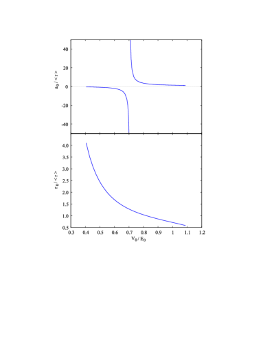
Figure 1: (Color online) Scattering length $a_{0}$ and effective range of the interaction $r_{0}$ as a function of the potential depth $V_{0}/E_{0}$, where the energy scale $E_{0}=\hbar^{2}/(m\langle r\rangle^{2})$.

Figure 2: (Color online) Momentum distributions $\rho_{k}$ (top) and the quasi-particle excitation spectra $E_{k}/\varepsilon_{F}$ (bottom) as a function of $k\equiv|\mathbf{k}|$, at fixed density ($k_{F}$) and various potential scattering lengths $a_{0}$, where $\varepsilon_{F}$ is the Fermi energy and $k_{F}\langle r\rangle\approx~{}0.37$.

Numerical solutions are found for an attractive short-range interaction, described by a Gaussian potential $V(r)=V_{0}\exp(-br^{2})$. We explore the BCS-BEC crossover by fixing the width of the potential $\langle r\rangle=2/\sqrt{\pi b}$ and varying the potential depth $V_{0}$, or implicitly the scattering length $a_{0}$ of the interaction. Fig. 1 depicts all the essential two-body physics of the problem. As the depth of the potential is increased from zero, the scattering length grows, diverging to negative infinity at the first appearance of a two-body bound state. On the bound-state side of the Feshbach resonance the scattering length re-emerges from positive infinity. Note that this procedure does not keep the effective range $r_{0}$ of the potential fixed. In the low-energy limit, the effective range $r_{0}$, like the scattering length $a_{0}$, can be determined from the phase shift

$$k\ \cot\delta_{0}\ =\ -\,\frac{1}{a_{0}}\ +\ \frac{1}{2}\,r_{0}\ k^{2}\>,$$ (13)

and is shown in Fig. 1. The variation of the effective range is small over the region of interest.

From now on, we shall focus on finite densities and the crossover to BCS that can occur in this regime. Like previous theoretical studies ref:sch_noz , we find that the momentum distribution $\rho_{k}$ at constant density smoothly evolves from the wave function of a molecule in momentum space at large positive $(a_{0}k_{F})^{-1}$ to a Fermi-like distribution at large negative $(a_{0}k_{F})^{-1}$, as depicted in Fig. 2 (top). During this transition, we see from Fig. 2 (bottom) that the quasi-particle excitation spectrum $E_{k}$ develops a minimum at finite momentum, signifying the BCS-BEC crossover point defined previously. Because the density is non-zero, though small, the crossover point occurs for positive $a_{0}k_{F}$, where a two-body molecular bound state has already formed.

The appearance of the minimum in the quasi-particle excitation spectrum at non-zero momentum is clearly evident in the quasi-particle density of states. As a function of momentum, the density of states is defined as

$$N_{k}=\frac{1}{\pi^{2}}\frac{k^{2}}{\left|\frac{\mathrm{d}E_{k}}{\mathrm{d}k}\right|}.$$ (14)

Thus, $N_{k}$ is singular whenever there is a stationary point in the excitation spectrum ($\mathrm{d}E_{k}/\mathrm{d}k=0$), except when $k=0$, where $N_{k}$ vanishes provided $\mathrm{d}E_{k}/\mathrm{d}k\rightarrow 0$ no faster than $k^{2}$. Fig. 3 shows how $N_{k}$ varies with scattering length at constant particle density. The energy minimum for $k>0$ shows up as a spike that migrates away from $k=0$ towards $k=k_{F}$ as $(a_{0}k_{F})^{-1}~{}\rightarrow~{}-\infty$, but the spike disappears when the energy minimum occurs at $k=0$. Thus, the BCS-BEC crossover is the point at which a spike first appears as we decrease $(a_{0}k_{F})^{-1}$.

A more straightforwardly measurable quantity may be the density of states as a function of energy

$$N_{E}=\frac{1}{\pi^{2}}\frac{k_{E}^{2}}{\left|\frac{\mathrm{d}E_{k}}{\mathrm{d}k}\right|_{E}}\>,$$ (15)

which is depicted in Fig. 4. Approximating the gap parameter $\Delta_{k}$ as a constant, the BCS regime has a singularity at finite momentum ($k=\sqrt{2m\mu}/\hbar$) of the form

$$N_{E}\simeq\frac{A}{\sqrt{E-\Delta}}\>,$$ (16)

where the amplitude is

$$A=\frac{1}{\pi^{2}\hbar^{3}}\sqrt{\frac{m^{3}\mu}{\Delta}}\>.$$ (17)

We see that the size of the singularity will increase the further we enter the BCS phase.

In the BEC limit, the density of states is zero at the energy minimum occurring at $k=0$, and deep within the BEC phase it has the following form close to the minimum

$$N_{E}\simeq\frac{\sqrt{2m^{3}}}{\pi^{2}\hbar^{3}}\sqrt{E-|\mu|}\>.$$ (18)

Figure 3: (Color online) Density of states $N_{k}$ (as a function of momentum), at fixed $k_{F}$ and various potential scattering lengths $a_{0}$, where $k_{F}\langle r\rangle\approx~{}0.37$.

Figure 4: (Color online) Density of states $N_{E}$ (as a function of energy), at fixed $k_{F}$, where $k_{F}\langle r\rangle\approx~{}0.37$, and various potential scattering lengths $a_{0}$.

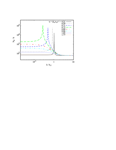
Figure 5: (Color online) Density of states $N_{k}$ (as a function of momentum), at fixed potential scattering length ($a_{0}/\langle r\rangle~{}=~{}2.4$), and various values of $k_{F}$.

As well as considering the BCS-BEC crossover at constant density arranged by tuning the interaction, we also examine the density-driven crossover at fixed interaction. Fig. 5 illustrates the density of states as a function of momentum for various particle densities, where we have chosen $a_{0}$ to be positive so that a molecular bound state exists. We observe the same disappearance of the spike in $N_{k}$ as $(a_{0}k_{F})^{-1}\rightarrow+\infty$ but, unlike Fig. 3, the extreme BCS limit occurs when $(a_{0}k_{F})^{-1}\rightarrow 0$ since this corresponds to infinite density. Note also that both Fig. 3 and 5 show $N_{k}/k\rightarrow$ const, as $(a_{0}k_{F})^{-1}\rightarrow+\infty$, so that the pair-breaking excitation spectrum has $(E_{k}-\delta E)\propto k^{2}$, where $\delta E$ is the binding energy of the molecule. This is exactly what we would expect for a non-interacting gas of Bose molecules.

Figure 6: (Color online) Momentum distribution of the condensate wave function, at fixed density ($k_{F}$) and various potential scattering lengths $a_{0}$, where $k_{F}\langle r\rangle\approx~{}0.37$ .

Finally, Fig. 6 shows the behavior of the condensate wave function throughout the crossover. Here we see the most pronounced features of the evolution from a molecular state to the BCS limit where pairing exists only on the Fermi surface.

IV Phase diagram and comparison with zero-range potential

Figure 7: Profiles of the chemical potential $\mu/\varepsilon_{F}$ as a function of $\eta=(a_{0}k_{F})^{-1}$. The points mark the BEC-BCS crossover.

A more complete understanding of the BCS-BEC crossover can be gained from considering the phase diagram for our finite-range potential. Figure 7 shows the variation of chemical potential $\mu/\varepsilon_{F}$ as a function of $(a_{0}k_{F})^{-1}$, for a set of different scattering lengths $a_{0}/\langle r\rangle$. On each curve we mark the position of the BCS-BEC crossover point, which we refer to as the “critical” pair ($\mu_{c}$, $k_{F\,c}$). The crossover point always occurs for $a_{0}>0$ and there is no density-driven crossover when $a_{0}<0$. Since the size of $a_{0}$ dictates the size of the two-body molecular bound state while $a_{0}>0$, the crossover point in Fig. 7 is driven to lower densities when $a_{0}$ is increased. As the zero-density limit ($k_{F\,c}$=0) is approached, the critical chemical potential $\mu_{c}/\varepsilon_{F}\rightarrow 0$, which is equivalent to the BCS-BEC crossover for a single-parameter potential initially discussed by Leggett. However, as $k_{F\,c}$ increases, the crossover point shifts to negative values of $\mu_{c}$ and larger $(a_{0}k_{F})^{-1}$.

It is useful to compare the results of our calculations with previous studies of the BCS-BEC crossover that involve single-parameter potentials. In the dilute or low-energy limit, where $k_{F}\langle r\rangle,\langle r\rangle/a_{0}\ll 1$, the effective interaction $U$ can be written as

$$U\ =\ \frac{4\pi a_{0}}{m}\>,$$ (19)

and it is independent of the details of the real interaction. Substituting $U$ for the potential and eliminating high energies, Eqs. (8) and (12) become, respectively

$$\int_{0}^{\infty}\ \mathrm{d}\varepsilon\ \sqrt{\varepsilon}\ \biggl{[}\frac{1}{\varepsilon}\ -\ \frac{1}{\sqrt{(\varepsilon-\tilde{\mu})^{2}+\tilde{\Delta}}}\biggr{]}\ =\ \pi\ \eta\>,$$ (20)

$$\int_{0}^{\infty}\ \mathrm{d}\varepsilon\ \sqrt{\varepsilon}\ \biggl{[}1\ -\ \frac{\varepsilon-\tilde{\mu}}{\sqrt{(\varepsilon-\tilde{\mu})^{2}+\tilde{\Delta}}}\biggr{]}\ =\ \frac{4}{3}\>,$$ (21)

where we have introduced the notations $\tilde{\mu}=\mu/\varepsilon_{F}$, $\tilde{\Delta}=\Delta/\varepsilon_{F}$, and $\eta=(a_{0}k_{F})^{-1}$. The above equations, first studied by Leggett ref:leg80 , are then solved for $\tilde{\mu}(\eta)$ and $\tilde{\Delta}(\eta)$. For obvious reasons, we will refer to these functions as “model independent” or “universal.”

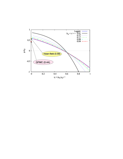
Figure 8: (Color online) Comparison with Leggett’s “universal” curve: We keep $k_{F}$ constant, and vary the scattering length $a_{0}$.

We first compare our results for $\tilde{\mu}(\eta)$ against Leggett’s predictions for the case where the scattering length $a_{0}$ is varied and the density is held fixed, as shown in Fig 8. On the Leggett curve, the BCS-BEC crossover point ($\mu=0$) occurs at $(a_{0}k_{F})^{-1}\approx 0.55$, and our numerical $\tilde{\mu}(\eta)$ converges to this universal curve as $k_{F}\langle r\rangle\rightarrow 0$. Since typical experimental parameters correspond to $k_{F}\langle r\rangle\simeq 0.04$, the ultracold atomic gases clearly lie on the Leggett curve and are well described by a single-parameter potential.

The value of $\mu/\varepsilon_{F}$ for $\eta=0$ is usually referred to as the “unitarity” limit unitarity ; bertsch ; carlson . In this limit one expects that all sensitivity to the detailed features of the interaction is lost schiff , and the system energy is determined entirely by the density. As a result, this limit is particularly sensitive to many-body correlation effects, and the Leggett curve predicts this value as being 0.59 (see also ref:ERM97 ). Recently, accurate calculations based on the Green’s Function Monte Carlo (GFMC) method carlson , have lowered the upper-bound on this result to ($0.44\pm 0.01$), which shows that beyond mean-field effects account for at least a 25% improvement in the binding energy over the mean-field result.

Figure 9: (Color online) Comparison with Leggett’s “universal” curve: The scattering length $a_{0}$ is held constant, the density ($k_{F}$) is varied.

Fig. 9 compares the numerical $\tilde{\mu}(\eta)$ with the universal curve for the case where the density is varied and $a_{0}/\langle r\rangle$ is fixed. Not surprisingly, the numerical $\tilde{\mu}(\eta)$ approaches the universal curve as scattering length increases, and we require $a_{0}/\langle r\rangle>18$ before $\tilde{\mu}(\eta)$ touches the universal curve. Furthermore, we see that no matter how large we make $a_{0}$, the universal curve breaks down in the region sufficiently close to $(a_{0}k_{F})^{-1}=0$. This point corresponds to infinite density, the BCS limit in the density-driven crossover, so we must always have $\tilde{\mu}(0)=1$, which is consistent with our numerical results. If we consider $\tilde{\mu}(\eta)$ for which $a_{0}/\langle r\rangle\approx 72$ we observe that it collapses onto the universal curve when $(a_{0}k_{F})^{-1}>0.3$. This translates into the condition $k_{F}\langle r\rangle<0.046$ for the universal equations to be valid, which is consistent with Fig. 8.

V Conclusion

In this paper we have performed a study of the BCS-BEC crossover, at zero temperature, in the single-channel model, using a realistic effective interaction. In the mean-field approximation the crossover is described using a variational wave function, which interpolates smoothly between the BEC and BCS limits. We find that the crossover point always lies on the side of the Feshbach resonance where a molecular bound state exists at zero density, and that it converges to that of a single-parameter potential in the low density limit. Moreover, our results reproduce the usual Leggett picture in the limit of a dilute Fermi gas, as expected. By using a potential of finite range, we have shown that the crossover for typical experimental parameters in ultracold atomic Fermi gases can be described by a zero-range, single-parameter potential. We emphasize that a clear signature of the crossover point appears in the density of states, which could be measured spectroscopically ref:TZ00 .

The mean-field description of the single-channel model presented here is not entirely satisfactory. As described above, recent GFMC results provide an upper value for the energy density in the dilute limit ($\eta=0$), which represents a 25% improvement over the Leggett limit. Therefore, additional work is required in order to include next-to-leading order effects in a quantitative way, and study the changes (or lack thereof) in the features of the BEC-BCS crossover. Approximations schemes based on the two-particle irreducible effective action 2PI are readily available in quantum field theory where they have been recently employed to describe the dynamics of a system out of equilibrium, and the dynamics of phase transitions BVA . Work is currently under way in order to apply such methods to the study of the BEC-BCS crossover based on the Hamiltonian (1).

The single-channel model is of course a simplification of detailed models for the Feshbach resonance which include the resonance explicitly, either as a boson (the Fermi-Bose model fermibose ) or more generally as three-level  3level or four-level fermi systems. The Fermi-Bose model, as well as models with even numbers of fermions, all have large regimes of parameter space where the resonance is sufficiently detuned from the open channel that high energy degrees of freedom can be integrated out in favor of an effective interaction between two species, recovering the model discussed in this paper. Close enough to resonance the detailed fermionic structure of the resonance may become important. Models where the Feshbach bound state shares a state with the open channel (relevant to ${}^{40}K$) are different, and do not reduce to an effective single channel model in a simple way3level . In future work, we will compare and contrast these different models manymodel using a generalization of the variational scheme given in this paper.

- (1) E. Tiesinga, B. J. Verhaar and H. T. C. Stoof, Phys. Rev. A 47, 4114 (1993).
- (2) C. A. Regal, C. Ticknor, J. L. Bohn, and D. S. Jin, Nature 424, 47 (2003); S. Jochim, M. Bartenstein, A. Altmeyer, G. Hendl, C. Chin, J. Hecker Denschlag and R. Grimm, Science 302, 2101 (2003); M. Greiner, C. A. Regal, and D. S. Jin, Nature 426, 537 (2003); M. W. Zwierlein, C. A. Stan, C. H. Schunck, S. M. F. Raupach, S. Gupta, Z. Hadzibabic and W. Ketterle, Phys. Rev. Lett. 91, 250401 (2003); T. Bourdel, L. Khaykovich, J. Cubizolles, J. Zhang, F. Chevy, M. Teichmann, L. Tarruell, S.J.J.M.F. Kokkelmans, and C. Salomon, Phys. Rev. Lett. 93, 050401 (2004).
- (3) C. A. Regal, M. Greiner, and D. S. Jin, Phys. Rev. Lett. 92, 040403 (2004); M. W. Zwierlein, C. A. Stan, C. H. Schunck, S. M. F. Raupach, A. J. Kerman, and W. Ketterle, Phys. Rev. Lett. 92, 120403 (2004).
- (4) A.J. Leggett, in Modern Trends in the Theory of Condensed Matter, edited by A. Pekalski and R. Przystawa (Springer-Verlag, Berlin, 1980).
- (5) M. Randeria, in Bose-Einstein Condensation, edited by A. Griffin, D. W. Snoke, and S. Stringari (Cambridge University Press, Cambridge, 1995).
- (6) J. R. Schrieffer, Theory of Superconductivity, (Benjamin/Cummings, Reading, 1964)
- (7) C. Comte and P. Nozières, J. Physique 43, 1069 (1982); P. B. Littlewood and X. J. Zhu, Physica Scripta T68, 56 (1996).
- (8) P. Nozières and S. Schmitt-Rink, J. Low Temp. Phys. 59, 195 (1985).
- (9) H. Heiselberg, Phys. Rev. A 63, 043606 (2001); R. Combescot, Phys. Rev. Lett. 91, 120401 (2003).
- (10) G. A. Baker, Phys. Rev. C 60, 054311 (1999); T. Papenbrock and G. F. Bertsch, Phys. Rev. C 59, 2052 (1999).
- (11) J. Carlson, S.-Y. Chang, V. R. Pandharipande, and K. E. Schmidt, Phys. Rev. Lett. 91, 050401 (2003).
- (12) L. I. Schiff, Quantum Mechanics, McGraw-Hill, New York (1968).
- (13) J. R. Engelbrecht, M. Randeria, and C.A.R. Sá de Melo, Phys. Rev. B 55, 15153 (1997).
- (14) J. Stenger, S. Inouye, A. P. Chikkatur, D. M. Stamper-Kurn, D. E. Pritchard, and W. Ketterle, Phys. Rev. Lett. 82, 4569 (1999); P. Törmä and P. Zoller, Phys. Rev. Lett. 85, 487 (2000); T. Bourdel, J. Cubizolles, L. Khaykovich, K. M. F. Magalhaes, S. J. J. M. F. Kokkelmans, G. V. Shlyapnikov,and C. Salomon, Phys. Rev. Lett. 91, 020402 (2003); L. Viverit, S. Giorgini, L. P. Pitaevskii, and S. Stringari, Phys. Rev. A 69, 13607 (2004).
- (15) J. M. Luttinger and J. C. Ward, Phys. Rev. 118, 1417 (1960); G. Baym, Phys. Rev. 127, 1391 (1962); H. D. Dahmen and G. Jona Lasino, Nuovo Cimento, 52A, 807 (1962); J. M. Cornwall, R. Jackiw and E. Tomboulis, Phys. Rev. D 10, 2428 (1974).
- (16) K. B. Blagoev, F. Cooper, J. F. Dawson and B. Mihaila, Phys.Rev. D. 64, 125003 (2001); F. Cooper, J. F. Dawson and B. Mihaila, Phys. Rev. D 67, 051901(R) (2003); F. Cooper, J. F. Dawson, and B. Mihaila, Phys. Rev. D 67, 056003 (2003); B. Mihaila, Phys. Rev. D 68, 36002 (2003) [hep-ph/0303157].
- (17) M. Holland, S. J. J. M. F. Kokkelmans, M. L. Chiofalo and R. Walser, Phys. Rev. Lett. 87, 120406 (2001); E. Timmermans, K. Furuya, P. W. Milonni and A. K. Kerman, Phys. Lett. A 285, 228 (2001); Y. Ohashi and A. Griffin, Phys. Rev. Lett. 89, 130402 (2002).
- (18) M. M. Parish, B. Mihaila, B. D Simons, and P. B. Littlewood, cond-mat/0409756.
- (19) B. Mihaila, M. M. Parish, E. M. Timmermans, K. B. Blagoev, and P. B. Littlewood, [in preparation].