Time Scale for Magnetic Reversal at The Topological Non–connectivity Threshold

Abstract

Anisotropic classical Heisenberg models with all-to-all spin coupling display a Topological Non–connectivity Threshold (TNT) for any number $N$ of spins. Below this threshold, the energy surface is disconnected in two components with positive and negative total magnetizations respectively, so that magnetization cannot reverse its sign and ergodicity is broken, even at finite $N$. Here, we solve the model in the microcanonical ensemble, using a recently developed method based on large deviation techniques, and show that a phase transition is present at an energy higher than the TNT energy. In the energy range between the TNT energy and the phase transition, magnetization changes sign stochastically and its behavior can be fully characterized by an average magnetization reversal time. The time scale for magnetic reversal can be computed analytically, using statistical mechanics. Numerical simulations confirm this calculation and further show that the magnetic reversal time diverges with a power law at the TNT threshold, with a size dependent exponent. This exponent can be computed in the thermodynamic limit ($N\to\infty$), by the knowledge of entropy as a function of magnetization, and turns out to be in reasonable agreement with finite $N$ numerical simulations. We finally generalize our results to other models: Heisenberg chains with distance dependent coupling, small 3D clusters with nearest neighbor interactions, metastable states. We conjecture that the power-law divergence of the magnetic reversal time scale might be a universal signature of the presence of a TNT.

I Introduction

Statistical mechanics deals with systems containing a very large number ($10^{23}$) of interacting particles. Nowadays, as the experimental investigation of few-atom systems is becoming possible, the analysis of small systems raises fundamental questions Gross , and the problem of a statistical description of few-body systems with strong nonlinear interaction is a subject of current research chaos . Unfortunately we are still far from understanding what are the conditions for a few-body system to reach, if any, an equilibrium, and how to describe it in the same way as statistical mechanics provides a powerful description of large systems. For instance, even the existence of temperature at the nanoscale has been recently questioned in Ref. nano .

It has been recently shown that, for a Heisenberg model with all-to-all coupling, there exists a specific energy threshold below which total magnetization cannot change its sign, even when the number of spins is finite jsp . This ergodicity breaking phenomenon has been related to the existence of a Topological Non-connectivity Threshold (TNT) of the energy surface. This type of ergodicity breaking at finite $N$ is different from the $N\to\infty$ ergodicity breaking in a standard Ising model below the critical temperature. The existence of this threshold is not restricted to the infinite range coupling case. It is also present when the interaction among Heisenberg spins decays as $R^{-\alpha}$, where $R$ is the distance between two spins. It has been indeed proved brescia that, for a $d-$dimensional system, the ratio of the disconnected portion of the energy range with respect to the total energy range tends to zero in the thermodynamic limit for $\alpha>d$ (short range interactions) while it remains finite for $\alpha<d$ (long range interactions). On the other hand, although the mean-field (all-to-all) type of spin coupling might appear unphysical, magnetic systems can be realized, using modern experimental techniques cornell , which are well described by Heisenberg–like Hamiltonians with an infinite range term. Moreover, when the range of the interaction is of the same order of the size of the system, all-to-all coupling may be a meaningful first order approximation Gross ; thebibble . This could be the case for small systems used in current nano-technology, which requires to deal with systems made of a few dozens of particles. Otherwise, all-to-all coupling is relevant for macroscopic systems with long range interactions, like gravitational and unscreened Coulomb systems thebibble .

We address in this paper the issue of providing a theoretical framework to calculate the magnetization reversal time for the mean-field anisotropic Heisenberg model in a magnetic field, in which a finite number $N$ of spins interact with all-to-all couplings. We have already stressed that below the TNT the total magnetization cannot reverse its sign, thus magnetization does not relax to its equilibrium value. In this paper we will answer the following questions: $i)$ Above the TNT, does the magnetization reverse its sign? If so, on which time scale? $ii)$ What is the relevance of the TNT in a system with a standard magnetic phase transition? Thus, the aim is to explain the main physical effects associated with the TNT, and how it affects the phase transition appearing in this model at a higher energy. The latter is studied in the microcanonical ensemble, applying a recently developed solution method of mean-field Hamiltonians based on large-deviation theory thierry . We study in detail, numerically and analytically, the time scale for magnetization reversal. At the TNT, the reversal time diverges as a power law, with a characteristic exponent proportional to the number of spins $N$. Based on analytical calculations, we expect this property to be universal. Finally, we extend some of the results obtained for all-to-all coupling to other models: chains with distance dependent couplings and small clusters with nearest neighbor interactions. We show the existence of the TNT also in these cases, and we present strong evidence for the power law divergence of the reversal time.

II The Model

The Hamiltonian of the model is

$$H=B\sum_{i=1}^{N}S^{z}_{i}+\frac{J}{2}\sum_{i=1}^{N}\sum_{j\neq i}(S_{i}^{x}S_{j}^{x}-S_{i}^{y}S_{j}^{y}),$$ (1)

where $\vec{S}_{i}=(S_{i}^{x},S_{i}^{y},S_{i}^{z})$ is the spin vector with continuous components, $N$ is the number of spins, $B$ is the rescaled external magnetic field strength and $J$ the all-to-all coupling strength (the summation is extended over all pairs). Let us also define

$$m_{x,y,z}=\frac{1}{N}\sum_{i=1}^{N}S_{i}^{x,y,z},$$

as the components of the total magnetization of the system. Due to the anisotropy of the coupling, the system has an easy–axis of the magnetization along the $y$ direction (the easy–axis of the magnetization is defined by the direction of the magnetization in the minimal energy configuration of the system). The equations of motion are derived in a standard way from Hamiltonian (1), and we obtain:

$$\left\{\begin{array}[]{ccc}\dot{S}_{i}^{x}&=&-BS_{i}^{y}-JS_{i}^{z}\sum_{\langle j\rangle}S_{j}^{y}\\ \\ \dot{S}_{i}^{y}&=&BS_{i}^{x}-JS_{i}^{z}\sum_{\langle j\rangle}S_{j}^{x}\\ \\ \dot{S}_{i}^{z}&=&J\sum_{\langle j\rangle}(S_{i}^{y}S_{j}^{x}+S_{i}^{x}S_{j}^{y}).\end{array}\right.$$ (2)

The total energy $E=H$ and the spin moduli $|\vec{S}_{i}|^{2}=1$ are constants of the motion. Dynamics, already studied in a similar model jsp ; num , is characterized by chaotic motion (positive maximal Lyapunov exponent) for not too small energy values and spin coupling constants. For $J=0$ the model is exactly integrable, while for generic $J$ and $B$ there is a mixed phase space with prevalently chaotic motion for $|E|\lesssim JN$.

III The two thresholds

We will now show the existence of two distinct thresholds in this model: first we derive analytically the Topological Non–connectivity Threshold (TNT), then we will present the microcanonical analysis and the analytical evaluation of the statistical threshold, at which a second order phase transition occurs in the $N\rightarrow\infty$ limit.

III.1 The Topological Non–connectivity Threshold

The phase space of the system is topologically disconnected below a given energy density $\epsilon_{dis}$, which can be obtained as in Ref. jsp ; phd . From symmetry considerations, both positive and negative regions of $m_{y}$ exist on the same energy surface. Indeed the Hamiltonian is invariant under a rotation of $\pi$ around the $z$ axis for which $S_{i}^{y}\rightarrow-S_{i}^{y}$ and $S_{i}^{x}\rightarrow-S_{i}^{x}$. Switching dynamically from a negative $m_{y}$ value to a positive one requires, for continuity, to pass through $m_{y}=0$. Hence, for all energy values above

$$\epsilon_{dis}=\mbox{Min}[H/N\ |\ m_{y}=0]$$

magnetization reversal is possible, while below this value magnetization cannot change sign.

Hamiltonian (1) can be written as follows:

$$H=BNm_{z}+\frac{J}{2}N^{2}\left(m_{x}^{2}-m_{y}^{2}\right)+\frac{J}{2}\sum_{i}(S_{i}^{y})^{2}-(S_{i}^{x})^{2}.$$ (3)

The Topological Non-connectivity Threshold (TNT) is defined as the minimum of the Hamiltonian under the $N+1$ constraints:

$$a)\,(S_{i}^{x})^{2}+(S_{i}^{x})^{2}+(S_{i}^{x})^{2}=1$$ (4)

$$b)\,m_{y}=0.$$ (5)

Instead of solving the constrained problem, we simplify it by calculating the absolute minimum of

$$F=BNm_{z}-\frac{J}{2}\sum[(S_{i}^{x})^{2}-(S_{i}^{y})^{2}].$$

If the minimal solution satisfies both $m_{x}=0$ and $m_{y}=0$, the problem is equivalent to the original one. Conditions (4) are taken into account setting:

$$S_{i}^{z}=\cos\theta_{i},\ S_{i}^{x}=\sin\theta_{i}\cos\phi_{i},\ S_{i}^{y}=\sin\theta_{i}\sin\phi_{i}~{}.$$

Taking the derivatives of $F$ we obtain:

$$\frac{\partial{F}}{\partial\phi_{i}} = J\sin^{2}\theta_{i}\cos\phi_{i}\sin\phi_{i}=0$$ (6)

$$\frac{\partial{F}}{\partial\theta_{i}} = \sin\theta_{i}[B+J\cos\theta_{i}\cos^{2}\phi_{i}]=0~{}.$$ (7)

If $B>J$, Eq. (7) has the solution, $\sin\theta_{i}=0$, that also satisfies Eq. (6). It corresponds to all spins lying along the $z$-axis and

$$\epsilon_{dis}=-B~{}.$$ (8)

If $B<J$, then from Eq. (7) we have two possible solutions for each $i$:

• $\theta_{i}=\pi$;

• $\sin\phi_{i}=0$ and $\cos\theta_{i}=-B/J$

Let us define $0\leq n_{z}\leq N$ as the number of spins satisfying condition 1) above. Then

$$F(n_{z})=\frac{n_{z}}{2J}\left(B-J\right)^{2}-N\left(\frac{B^{2}}{2J}+\frac{J}{2}\right),$$

so that the minimum is reached for $n_{z}=0$ or $\cos\theta_{i}=-B/J$ and $\sin\phi_{i}=0$ for all $i$. This in turn implies $m_{y}=0$ and, for $N$ even, $m_{x}=0$ (choosing for instance $\phi_{i}=\pi/2$ for $i=1,N/2$ and $\phi_{i}=-\pi/2$ for $i=N/2+1,N$). Then we have (for $N$ even):

$$\epsilon_{dis}=-\left(\frac{B^{2}}{2J}+\frac{J}{2}\right)~{}.$$ (9)

Summarizing, we get odd ,

$$\epsilon_{dis}=\left\{\begin{array}[]{lll}\displaystyle&-B~{}{\rm for}~{}J\leq B{}\\ &\\ \displaystyle&-(\frac{B^{2}}{2J}+\frac{J}{2})~{}{\rm for}~{}J>B.\end{array}\right.$$ (10)

The existence of $\epsilon_{dis}$ does not represent a sufficient condition in order to demagnetize a sample for $\epsilon>\epsilon_{dis}$. As it will be shown in Sec. IV.2, regular structures indeed appear in some cases, preventing most trajectories to cross the $m_{y}=0$ plane.

III.2 The Statistical Threshold: phase transition

We now determine the statistical phase-transition energy of the model in the microcanonical ensemble. To keep the calculations easy, we will first neglect the term $J/2\sum_{i}(S_{i}^{y})^{2}-(S_{i}^{x})^{2}$ in (3). We will show later how to take into account this term. In order to facilitate the calculations, we will also set

$$\epsilon \rightarrow \epsilon/B$$

$$I \rightarrow \frac{JN}{B}~{}.$$ (11)

Thus we can consider the following Mean-Field Hamiltonian:

$$H_{MF}=N\left[m_{z}+\frac{I}{2}\left(m_{x}^{2}-m_{y}^{2}\right)\right],$$ (12)

Note that this mean field limit is formally identical to phenomenological single spin Hamiltonians used to model micromagnetic systems chud .

Using this simplified Hamiltonian, we can calculate the entropy, counting the number of microscopic configurations associated with given values of $m_{x}$, $m_{y}$ and $m_{z}$, independently of the energy of the system. This can be done using Cramér theorem, a basic tool of Large Deviation Theory Dembo . Each single spin is characterized by two angles $\theta$ and $\phi$, such that $S_{z}=\cos\theta$, $S_{x}=\sin\theta\cos\phi$, $S_{y}=\sin\theta\sin\phi$. We calculate the function

$$\Psi(\lambda_{x},\lambda_{y},\lambda) = \frac{1}{4\pi}\int_{0}^{\pi}\sin\theta\;d\theta\int_{0}^{2\pi}d\phi~{}e^{\lambda\cos\theta}$$ (13)

$$e^{\lambda_{x}\sin\theta\cos\phi+\lambda_{y}\sin\theta\sin\phi}~{}.$$

We then get the entropy $s(m_{x},m_{y},m_{z})$ through a Legendre-Fenchel transform of $\ln\Psi$:

$$s(m_{x},m_{y},m_{z}) = -\sup_{\lambda_{x},\lambda_{y},\lambda}\left[\lambda_{x}m_{x}+\lambda_{y}m_{y}+\lambda m_{z}\right.$$ (14)

$$\left.-\ln\Psi(\lambda_{x},\lambda_{y},\lambda)\right]~{}.$$

This calculation gives us an approximate expression for the probability $P(m_{x},m_{y},\epsilon)$, which describes the system for each energy:

$$P(m_{x},m_{y},\epsilon)\propto\exp{(Ns(m_{x},m_{y},m_{z}=\epsilon-\frac{I}{2}(m_{x}^{2}-m_{y}^{2})))}~{}.$$ (15)

Integrating over $m_{x}$, one gets the marginal probability distribution $P(m_{y},\epsilon)$. We define the paramagnetic (resp. ferromagnetic) phase by a probability distribution $P(m_{y},\epsilon)$ which is single peaked around $m_{y}=0$ (resp. double peaked). To locate the statistical phase transition energy $\epsilon_{stat}$, we assume that the transition is second order; it is then sufficient to study the entropy around $m_{y}=0$. We will also set $m_{x}=0$, since it is easy to see that a non-zero $m_{x}$ would only decrease the entropy for negative energy states; thus these states with non zero $m_{x}$ have little influence. Physically, the picture is the following: the negative energy has to be absorbed by either a non-zero $m_{z}$, or a non-zero $m_{y}$ or both. For small negative energies, it is entropically favorable to decrease a bit $m_{z}$, since it has a linear effect on the energy. For negative enough energies however, it costs much entropy to decrease $m_{z}$ further, so that a non-zero $m_{y}$ is favored, this is the phase transition. As a small $m_{y}$ results in a small $\lambda_{y}$, we develop $\Psi$ and $\ln\Psi$ up to second order in $\lambda_{y}$:

$$\Psi(\lambda_{y},\lambda) \simeq \frac{\sinh\lambda}{\lambda}+\frac{\lambda_{y}^{2}}{2}\frac{\lambda\cosh\lambda-\sinh\lambda}{\lambda^{3}}$$ (16)

$$\ln\Psi(\lambda_{y},\lambda) \simeq \ln\left(\frac{\sinh\lambda}{\lambda}\right)+\frac{\lambda_{y}^{2}}{2}\frac{\lambda\cosh\lambda-\sinh\lambda}{\lambda^{2}\sinh\lambda}~{}.$$ (17)

The maximization over $\lambda$ and $\lambda_{y}$ yields the equations:

$$m_{z} = \lambda\phi(\lambda)+\frac{\lambda_{y}^{2}}{2}\phi^{\prime}(\lambda)$$ (18)

$$m_{y} = \lambda_{y}\phi(\lambda)~{},$$ (19)

where

$$\phi(\lambda)=\frac{\lambda\cosh\lambda-\sinh\lambda}{\lambda^{2}\sinh\lambda}~{}.$$ (20)

From Eq. (18), we write $\lambda=\lambda_{0}+a_{2}\lambda_{y}^{2}$, where $\lambda_{0}$ is defined implicitly by

$$m_{z}=\lambda_{0}\phi(\lambda_{0})~{},$$ (21)

and $a_{2}$ is a coefficient. We then compute the entropy up to second order in $m_{y}$:

$$s(m_{y},\epsilon)=-\frac{m^{2}_{y}}{2\phi(\lambda)}-\lambda_{0}\left(m_{z}\right)+\ln\left(\frac{\sinh\lambda_{0}}{\lambda_{0}}\right)~{};$$ (22)

note that the terms with $a_{2}$ canceled. Using energy conservation $m_{z}=\epsilon+Im_{y}^{2}/2$, we obtain the entropy $s(m_{y};\epsilon)$ as a function of $m_{y}$ alone, $\epsilon$ being now a parameter. The equation for $\lambda_{0}$ is:

$$\epsilon+\frac{I}{2}m^{2}_{y}=\lambda_{0}\phi(\lambda_{0})~{}.$$ (23)

We then write $\lambda_{0}=\mu+m^{2}_{y}\mu^{2}$, with $\epsilon=\mu\phi(\mu)$, and substitute into Eq. (22), to get $s(m_{y};\epsilon)$ up to second order in $m_{y}$:

$$s(m_{y},\epsilon)=-\mu\epsilon+\ln\left(\frac{\sinh\mu}{\mu}\right)-m^{2}_{y}\left(\frac{1}{2\epsilon}+\frac{I}{2}\right)~{}.$$ (24)

The vanishing of the second derivative in $m_{y}=0$ yields the critical energy: $\epsilon_{stat}=-1/I$, which can be expressed in the old variables, see Eq. (11):

$$\epsilon_{stat}=-\frac{B^{2}}{JN}.$$ (25)

At this threshold entropy has a maximum in $m_{y}=0$, with vanishing second derivative. In the thermodynamic limit the second derivative of the entropy as a function of $\epsilon$ becomes discontinuous in $\epsilon_{stat}$, indicating that a true second order phase transition occurs at $\epsilon_{stat}$, for $N\to\infty$. This analytically calculated value of $\epsilon_{stat}$ is in reasonable agreement with numerical results obtained using the full Hamiltonian (1).

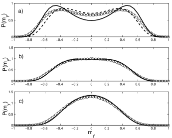
Figure 1: Comparison of the distributions $P(m_{y})$ obtained analytically (solid lines) and numerically (open circles). All plots are for $N=6$ spins, a coupling $J=1/3$ and a field $B=1$. From top to bottom, the energy per spin is $\epsilon=-0.7$ (ferromagnetic phase), $\epsilon=-0.5$ (close to the phase transition), and $\epsilon=-0.3$ (paramagnetic phase). In panel $a)$ the dashed line shows the improved analytical calculations in which the non-mean field terms are taken into account.

The corresponding probability distribution $P(m_{y},\epsilon)$ obtained from the mean field Hamiltonian (12), should be compared with that obtained (numerically) from the full Hamiltonian (1), for instance by sampling of the phase space. Results are shown in Fig. 1. As one can see the agreement is quantitatively good in the paramagnetic phase, but only qualitatively correct in the ferromagnetic phase; here the double peaked shape is correct, but the details are significantly off.

The inaccuracy of the calculation may come from both the small value of $N$, and from the term $J/2\sum_{i}(S_{i}^{y})^{2}-(S_{i}^{x})^{2}$, which has been neglected till now. It can be included in the statistical analysis as follows. The Hamiltonian depends now on another global quantity, $\Delta=\langle(S_{i}^{x})^{2}-(S_{i}^{y})^{2}\rangle$. It is possible to include it in the large deviation calculation; Eq. (13) is modified into:

$$\tilde{\Psi}(\lambda_{x},\lambda_{y},\lambda,\mu)=\frac{1}{4\pi}\int_{0}^{\pi}\sin\theta\;d\theta\int_{0}^{2\pi}d\phi\ e^{\lambda\cos\theta}\cdot$$

$$e^{\lambda_{x}\sin\theta\cos\phi+\lambda_{y}\sin\theta\sin\phi}\ e^{\mu\sin^{2}\theta(\cos^{2}\phi-\sin^{2}\phi)}.$$ (26)

One proceeds by writing a probability distribution $P(m_{x},m_{y},m_{z},\Delta)\propto\exp(Ns(m_{x},m_{y},m_{z},\Delta))$, taking into account the energy conservation $m_{z}=\epsilon-I(m_{x}^{2}-m_{y}^{2})/2+J\Delta/2$ (for $B=1$), and integrating over $m_{x}$ and $\Delta$ to obtain $P(m_{y},\epsilon)$. This last step has to be carried out numerically, and no simple expression as (25) is available any more. A comparison with a numerical investigation of the phase space shows that the additional term has a significant contribution; the $P(m_{y})$ we obtained in the ferromagnetic phase improves on the mean field calculation, see Fig. 1. We conclude that the remaining discrepancies come from the small value of $N$ ($N=6$ on Fig. 1).

Let us finally remark that in this statistical framework, the TNT energy, $\epsilon_{dis}$, can be recovered as the energy such that $s(0,\epsilon_{dis})=-\infty$. From Eqs. (21,24) with $m_{y}=0$, it is easy to get $\epsilon_{dis}=-1$; this implies, using Eq. (11), $\epsilon_{dis}=-B$, which is the same as in Eq. (10) in the limit $N\to\infty$ for $J<B$.

IV Time Scale for Magnetic Reversal

In the following, we will study the dynamics of the full Hamiltonian (1), which, at variance with (12), is non–integrable and can display chaotic motion. Let us first notice that in the large $N$ limit the minimal energy can be easily estimated (see Appendix A) as

$$\epsilon_{min}=\left\{\begin{array}[]{lll}\displaystyle&-\frac{B^{2}}{2JN}-\frac{JN}{2}\ {\rm~{}~{}~{}for}\qquad J\geq\frac{B}{N}\\ &\\ \displaystyle&-B\quad{\rm~{}~{}~{}~{}~{}~{}~{}~{}for}\qquad J<\frac{B}{N}.\end{array}\right.$$ (27)

From Eqs. (27,25,10) we have that if $J>B/N$ then $\epsilon_{stat}>\epsilon_{dis}>\epsilon_{min}$. In what follows we will restrict our consideration to the region of parameters for which these three thresholds are different.

The two thresholds, $\epsilon_{dis}$ and $\epsilon_{stat}$, define three energy regions which show different dynamical and statistical properties:

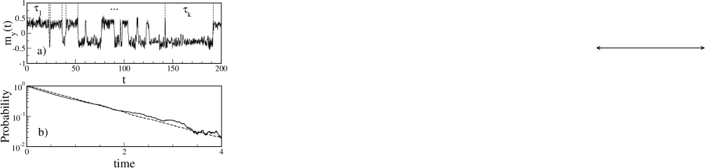
Figure 2: In this figure, all data refer to the $N=6$, $B=1$, $J=3$ case. a) Magnetization $m_{y}$ vs time. Reversal times (times between neighbor zeros of $m_{y}$ have been indicated as $\tau_{1},\ldots,\tau_{k}$. b) Solid line : probability distribution of reversal times versus the normalized time $\tau/\langle\tau\rangle$, for $1$ trajectory and $10^{4}$ different crossings. Dashed line : probability distribution of relaxation times $P=\frac{P_{+}(t)-1/2}{P_{+}(0)-1/2}$ vs $2t/\langle\tau\rangle$. As initial condition we choose $P_{+}(0)=1$ and $10^{4}$ different initial conditions.

1) For $\epsilon<\epsilon_{dis}$, the probability distribution of $m_{y}$ $P(m_{y})$ has two separate peaks, with $P(m_{y}=0)=0$, so that $m_{y}$ cannot change sign in time.

2) For $\epsilon_{stat}\leq\epsilon\leq 0$, $m_{y}$ quickly changes sign in time and $P(m_{y})$ is peaked at $m_{y}=0$.

3) For $\epsilon_{dis}<\epsilon<\epsilon_{stat}$, the probability distribution is doubly peaked around the most probable values of the magnetization. These two peaks are not separated and $P_{0}\equiv P(m_{y}=0)\neq 0$. What actually happens dynamically depends on the relative strength of the coupling $J$ with respect to $B$. More specifically we can characterize two different behaviors, chaotic and quasi-integrable.

IV.1 Chaotic Regime

IV.1.1 Time scale for magnetic reversal and relaxation

For $J$ big enough (fully chaotic regime) the behavior of $m_{y}(t)$ resembles a random telegraph noise tel , Fig. 2a): magnetization switches stochastically between its two most probable values, reversing its sign at random times. If we sample the magnetization reversal times, $\tau_{k}$, defined as the time interval between two crossings of $m_{y}=0$, we find that they follow a Poissonian distribution with average $\langle\tau\rangle$. Such distribution of the reversal times is a consequence of strong chaos: the system looses its memory due to sensitivity to initial conditions and the reversal probability per unit time, $\lambda=1/\langle\tau\rangle$, becomes time independent.

Since the magnetization reverses its sign randomly, any initial macroscopic sample with $m_{y}\neq 0$, will relax to an equilibrium distribution with a vanishing average magnetization. In order to characterize quantitatively the relaxation process, we introduce the probability to have a positive magnetization, $P_{+}(t)$, at time $t$. This is measured by considering an ensemble of $n$ initial conditions and counting, for each time $t$, the number of trajectories $n_{+}(t)$ for which $m_{y}>0$. At equilibrium we have $P_{+}=1/2$, in agreement with standard statistical mechanics considerations. Below $\epsilon_{dis}$, $P_{+}$ cannot change in time because the sign of $m_{y}$ remains the same for all trajectories. Above $\epsilon_{dis}$, $P_{+}(t)$ can change in time. Numerical results show that $P_{+}(t)$ decays exponentially to the equilibrium value $1/2$ and that the time scale for reaching the equilibrium value is independent of the initial probability distribution, $P_{+}(0)$, see Fig. 2b) (dashed line).

A simple statistical model can explain the qualitative features of this magnetic relaxation process. Let us start with an ensemble of $n$ initial conditions, of which $n_{+}$ with a positive magnetization and $n_{-}$ with a negative magnetization, such that $n=n_{+}+n_{-}$. Assuming that $m_{y}$ can take only two values, $+$ and $-$, we can write a pair of differential equation for the populations with positive and negative magnetizations:

$$\dot{n}_{+} = -\lambda n_{+}+\lambda n_{-}$$

$$\dot{n}_{-} = -\lambda n_{-}+\lambda n_{+}.$$

Where $\lambda$ is the reversal probability per unit time defined above. Defining $P_{+}=n_{+}/n$, we can solve these equations, obtaining

$$P_{+}(t)-\frac{1}{2}=(P_{+}(0)-\frac{1}{2})e^{-2\lambda t}.$$ (28)

$P_{+}(t)$ reaches the equilibrium value with a typical relaxation time $\tau=1/(2\lambda)$. This simple model predicts a magnetic relaxation time, $\tau$, proportional to the average magnetization reversal time, which checks pretty well with numerics (compare solid and dashed lines in Fig. 2b). Therefore, hereafter we will use indifferently the two concepts.

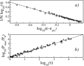
Figure 3: Panel $a)$ shows the scaling of the magnetic relaxation time $\tau$ for different values of $N$, for the case $B=0$, $J=3$. The relaxation time has been computed starting from an ensemble of $100$ different initial conditions. The dashed line is the linear fit: $\frac{1}{N}log(\tau)=0.075-0.82log(\epsilon-\epsilon_{dis})$. In panel $b)$ we show the times resulting from statistical mechanics, see Eq. (31), vs the dynamically computed relaxation times, for different $N$ values. $P_{max}/P_{0}$, the main ingredient of formula (31) is numerically determined for each energy density choosing $10^{6}$ points in a small energy interval. Symbols for the statistical times are as follows: $N=6$ (circle), $N=12$ (cross), $N=24$ (plus), $N=48$ (diamond). Dashed line is $y=x$.

Analyzing the magnetic relaxation times for all energies in the range $(\epsilon_{dis},\epsilon_{stat})$, we find that they grow exponentially with the number of spins for sufficiently large $N$, as expected for mean-field models. More remarkable is the power law divergence of relaxation time at the non–connectivity threshold. Numerical data are consistent with the following scaling law,

$$\tau\sim\left(\frac{1}{\epsilon-\epsilon_{dis}}\right)^{\alpha N}~{},$$ (29)

for which a theoretical justification will be given below. Eq. (29) is valid above the non-connectivity threshold and not too close to the statistical threshold $\epsilon_{stat}$. The comparison of this formula with numerical results is shown in Fig. 3.

To explain and substantiate these numerical findings, we now turn to an analytical estimate of the relaxation times, based on statistical mechanics. In Refs. tau1 ; tau2 , on the basis of fluctuation theory  landau ; gri , it has been argued that metastable states relax to the most probable state on times proportional to $\exp(N\Delta s)$ where $N$ is the number of degrees of freedom and $\Delta s$ is the specific entropic barrier. In our case $\exp(N\Delta s)$ is nothing but $P_{max}/P_{0}$, where $P_{max}$ is the value of $P(m_{y})$ for the most probable value of $m_{y}$, and $P_{0}=P(m_{y}=0)$. Thus, the exponential divergence as a function of $N$ shown in Fig. 3$a)$ is consistent with Refs. tau1 ; tau2 . These papers, however, did not study the behavior of $\tau$ at fixed $N$ in the neighborhood of the non–connectivity threshold. We perform this calculation in Appendix B, obtaining

$$\tau\sim 1/(\epsilon-\epsilon_{dis})^{\alpha N}~{},$$ (30)

with $\alpha=1$ generically, but $\alpha=3/4$ for $B=J=1$. This result is qualitatively correct (power law divergence, exponent proportional to $N$), and quantitatively reasonable. Indeed, numerical simulations give $\alpha\simeq 0.82$ (instead of $\alpha=1$) for $J\gg B$ and $B=0$ (see Fig. 3), and $\alpha\simeq 0.55$ (instead of $\alpha=3/4$) for $B=J=1$. We expect these qualitative features to be valid beyond the all-to-all coupling studied here, as it will be shown in Sec. V.

The calculations to evaluate $P_{max}/P_{0}$ rely on several approximations, the most doubtful being the large $N$ assumption (as seen also in Section III.2). Hence, despite the discrepancies in the exponents found above, the proportionality between $\tau$ and $P_{max}/P_{0}$ may still be valid, also for small $N$. To test this proportionality, we have calculated numerically the value of $P_{max}/P_{0}$, and we have found this value to be proportional to the relaxation time in any case. In particular, for the case $B=0$, we have found a very good fit setting

$$\tau=\frac{2}{J}\frac{P_{max}}{P_{0}}.$$ (31)

The $P_{max}/P_{0}$ factor in this formula represents the probability to cross the entropic barrier, and the $1/J$ factor can be heuristically associated with the typical time scale of the system (for $B=0$ the Hamiltonian is proportional to $J$). A deeper theoretical justification of this formula should be obtained in view of its success in describing the numerical results for different $N$ values (see Fig. 3$b)$).

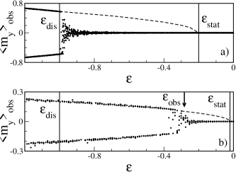
Figure 4: Time average of $m_{y}$ over the observational time $\tau_{obs}$ vs $\epsilon$ for different number of particles (a) $N=5$, (b) $N=50$, with fixed $J=B=1$. Each single point has been obtained taking the time average over the time intervals $\tau_{obs}=10^{5}$ (a) and $\tau_{obs}=10^{4}$ (b). Dashed curves indicate the equilibrium value of $m_{y}$, obtained from statistical mechanics. Vertical lines represent the non-connectivity and the statistical threshold respectively. The arrow in panel (b) indicates the energy value $\epsilon_{obs}$ of the chaotic driven phase transition due to the finite observational time.

IV.1.2 Chaotic Driven Phase Transition

Let us now answer the following question: if the measured values of the magnetization are given by the time average of the magnetization, for which energies the system will be found magnetized and for which unmagnetized?

From Eq. (29) and from the proportionality of the relaxation times and the reversal times, it is clear that the infinite time average of the magnetization will be zero above the TNT and different from zero below, due to the divergence of the reversal time. Nevertheless, the conclusion is different for a finite observational time $\tau_{obs}$. In Fig. 4 we show the time-averaged magnetization

$$\langle m_{y}\rangle_{obs}=\frac{1}{\tau_{obs}}\int_{0}^{\tau_{obs}}\ dt\ m_{y}(t)$$

vs the specific energy $\epsilon$ for $N=5$ (Fig. 4a) and $N=50$ (Fig. 4b) spins during a fixed observational time. While in (a) $\langle m_{y}\rangle_{obs}$ is zero just above $\epsilon_{dis}$, in (b) it vanishes at a value $\epsilon_{obs}$ located between $\epsilon_{dis}$ and $\epsilon_{stat}$. Indeed, if $\tau_{obs}\gg\tau$, the magnetization has time to flip between the two opposite states and, as a consequence, $\langle m_{y}\rangle_{obs}\simeq 0$. On the contrary, if $\tau_{obs}\ll\tau$ the magnetization keeps its sign and cannot vanish during $\tau_{obs}$. Defining an effective transition energy $\epsilon_{obs}$ from $\tau_{obs}=\tau(\epsilon_{obs})$, one gets, inverting Eq. (29), the value indicated by the vertical arrow in Fig. 4b. This is, a posteriori, a further demonstration of the validity of Eq. (29) for any $N$.

From a theoretical point of view, it is interesting to note that, for any fixed $N$, if the fully chaotic regime persists down to $\epsilon_{dis}$, $\epsilon_{obs}\to\epsilon_{dis}$ when $\tau_{obs}\to\infty$. On the other hand, in agreement with statistical mechanics, for any finite $\tau_{obs}$, $\epsilon_{obs}\to\epsilon_{stat}$ when $N\to\infty$. This implies that the limits $\tau_{obs}\rightarrow\infty$ and $N\rightarrow\infty$ do not commute. From the above considerations it follows that if $\tau_{obs}\to\infty$ at finite $N$, the threshold which distinguishes between a magnetized energy region and an unmagnetized one is $\epsilon_{dis}$ and not $\epsilon_{stat}$. We can thus consider $\epsilon_{dis}$ as the critical threshold at which a “dynamical” phase transition takes place: we call this transition a chaotic driven phase transition.

Let us finally note that, usually, for long-range interactions, the interaction strength is rescaled in order to keep energy extensive kaz . In our case this can be done setting $J=I/N$. With this choice of $J$ as $N\rightarrow\infty$, at fixed $I$, $J$ becomes much smaller than $B$, then a quasi–integrable regime sets in and Eq. (29) looses its validity (see Sec. IV.2). The presence of the TNT is therefore hidden.

IV.2 Quasi–integrable Regime

In this Section we will give numerical evidence of the quasi–integrable regime for $J<B$, in the energy region between $\epsilon_{dis}$ and $\epsilon_{stat}$. If the system dynamics is not in a fully chaotic regime, there are important consequences for reversal times. For instance reversal times strongly depend on initial conditions and Eq. (29) looses its validity:

In Fig. 5 we consider a system with different interaction strengths $J$ in order to enter a quasi-integrable regime (a and b) and a chaotic one (c and d). The energy in the two cases has been chosen such that the entropic barrier is roughly the same, see Fig. 5 $b)$ and $d)$. This means that, from a statistical point of view, both systems are characterized by roughly the same probability to jump over the barrier. Nevertheless, as one can see in panels $a)$ and $c)$ of Fig. 5, the behavior of the probability $P(t)=\frac{P_{+}(t)-1/2}{P_{+}(0)-1/2}$ significantly differs in the two cases. Such a big difference in the statistical properties of magnetic reversal times can be explained only by a drastic change in the dynamical properties of the system. Indeed, while Fig. 5a refers to a quasi–integrable regime, Fig. 5c refers to a fully chaotic regime. This cannot be explained by the different $J$ values, which, as we have shown in the previous Section, have only a linear effect on the reversal probability per unit time.

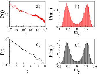
Figure 5: (Color online) Magnetic relaxation probability $P(t)=\frac{P_{+}(t)-1/2}{P_{+}(0)-1/2}$ and probability distributions of $m_{y}$ in the quasi–integrable ($J=0.5$, $\epsilon=-0.8$) (red panels a),b)), and chaotic ($J=3$,$\epsilon=-0.9$) (black panels c),d)) regimes. For both cases, $N=6$ and $B=1$. The specific energies for the two cases have been chosen in such a way that $P_{max}/P_{0}$ is the same (see panels $b)$ and $d)$). We compare $P(t)$ for the two different dynamical regimes. In the fully chaotic regime, panel $c)$, $P(t)$ decays exponentially with time $t$, and the average relaxation time is of order $1$. In the quasi–integrable regime, panel $a)$, the decay of $P(t)$ is much slower (observe the difference in the time axis scale).

To better understand the origin of this quasi-integrable regime, it is interesting to compare the dynamics obtained from the full Hamiltonian (3) with the dynamics obtained from the Mean-Field Hamiltonian (12). Taking into account the conservation of the total angular momentum $M^{2}=m_{x}^{2}+m_{y}^{2}+m_{z}^{2}$, a change of variable maps (12) onto a 2 degrees of freedom Hamiltonian; the dynamics of the global magnetization is then obviously integrable.

In Fig. 6 we show the projection of some trajectories on the $(m_{x},m_{y})$ plane. We considered the two different dynamical regimes described above. For definiteness, we vary $J$ but we choose the specific energy in order to keep the same value of $P_{max}/P_{0}\sim 20$. Let us first discuss Fig. 6a. Dark lines represent orbits of the Mean-Field Hamiltonian (12). The orbits of the macroscopic variable $\vec{m}=(m_{x},m_{y},m_{z})$ cover tori, since the Mean-Field Hamiltonian (12) is exactly integrable. Nevertheless, trajectories display different features: while trajectory $(1)$ crosses the line $m_{y}=0$, trajectory $(2)$ remains confined in the negative ($m_{y}<0$) branch belonging to the same energy surface. Two trajectories of the full Hamiltonian (3) and the same initial conditions are then considered, labeled by $(3)$ and $(4)$. As one can see these orbits stay for a long time sufficiently close to the Mean-Field orbits. Again, while $(4)$ displays a typical “ferromagnetic” behavior, $(3)$ is of “paramagnetic” nature. Both trajectories $(3)$ and $(4)$ have a positive maximal Lyapunov and are therefore chaotic. Upon increasing $J$, and keeping the same value of $P_{max}/P_{0}\sim 20$, we enter in the regime described by the lower panel in Fig. 6. In this case, as above, we show the orbit $(5)$ of the Mean-Field Hamiltonian (actually a “ferromagnetic” one). The corresponding orbit of the full Hamiltonian, $(6)$, is still characterized by a positive Lyapunov exponent and covers both branches, $m_{y}>0$ and $m_{y}<0$, thus inducing the demagnetization of the system. What is important to stress is that in this case the trajectories of the full Hamiltonian cover both the positive and the negative magnetization branch on the same energy surface. Having in mind the mechanism that produces the transition to global stochasticity in low-dimensional Hamiltonian systems Chirikov , we can conjecture that invariant curves, confining the motion, exist in the case of Fig. 6a. The breakdown of these invariant curves signals the transition to a globally chaotic motion. Of course, characterizing such a breakdown is an hard task, due to the high-dimensionality of the phase-space.

The determination of parameter regions in which the system is quasi–integrable or fully chaotic is still an open question. We can only make a few qualitative considerations. Let us consider Hamiltonian (3); it contains the sum of two terms: a mean-field integrable term plus the term $J/2\sum_{i}(S_{i}^{y})^{2}-(S_{i}^{x})^{2}$, which is responsible for the chaoticity of the system. The minimal specific energy of this term is $\epsilon_{chaos}\sim-J/2$. We can thus suppose that for $\epsilon<\epsilon_{chaos}$ the quasi–integrable regime prevails, while for $\epsilon>\epsilon_{chaos}$ a fully chaotic regime sets in. Thus, in order to have a fully chaotic regime in the energy region between $\epsilon_{dis}$ and $\epsilon_{stat}$, it is necessary that $\epsilon_{dis}>\epsilon_{chaos}$. This is always the case if $J>2B$ since for these values of $J$, $\epsilon_{dis}\sim\epsilon_{chaos}$. On the contrary, for $J<2B$ we expect a quasi–integrable regime between $\epsilon_{dis}$ and $\epsilon_{chaos}$, which should persist in the thermodynamic limit.

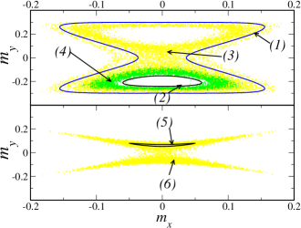
Figure 6: (Color online) Projections of the trajectories of $\vec{m}=(m_{x},m_{y},m_{z})$ over the $(m_{x},m_{y})$ plane for both the Mean-Field Hamiltonian (12) (heavy full lines : (1) blue and (2) black ) and the full Hamiltonian (3) (chaotically scattered dots (3) yellow and (4) green). In panel $a)$ ($J=0.2$, $\epsilon=-0.3$), the system is in a quasi–integrable regime. The orbits of the full Hamiltonian remain close to the orbits of the Mean-Field Hamiltonian for all the integration time considered ($10^{4}$). Note also that in the some of the orbits cross the $m_{y}=0$ line, thus demagnetizing the system, and some do not. In panel $b)$ ($J=3$, $\epsilon=-0.32$) the system is in a highly chaotic regime. In this case the orbit of the full Hamiltonian (6-yellow) does not remain close to the one of the Mean-Field Hamiltonian (5-black) and covers most of the available phase–space. The integration time is, also in this case, $10^{4}$.

V Other Models

Till now, we have concentrated our analysis on a spin system with all-to-all anisotropic coupling. The results obtained concerning the TNT and the time scales for magnetic reversal can be extended to more general situations. In this Section, we consider two possible generalizations, and discuss how our results can be extended to: $i)$ distance dependent interactions and $ii)$ metastable states.

$i)$ Distance dependent coupling. In Ref.brescia it has been considered a spin coupling which decays with the distance as $R^{-\alpha}$. It is possible to prove that in the $N\to\infty$ limit, for $\alpha<d$, a finite portion $r$ of the energy range corresponds to a disconnected energy surface. For $\alpha>d$, this portion vanishes in the $N\to\infty$ limit. For finite $N$, however, a well defined non connectivity threshold $\epsilon_{dis}>\epsilon_{min}$ exists in both the short and the long case when the anisotropy of the coupling induces an easy–axis of the magnetization. Numerical simulations support the conjecture that the behavior of the average magnetization reversal time is qualitatively similar to the $\alpha=0$ case. A power law divergence of the average reversal time when $\epsilon$ approaches $\epsilon_{dis}$ is observed, see Fig. 7.

More realistic models of micromagnetic systems include 3D clusters of spins interacting only with their neighbors. Again, for large $N$, the non connectivity threshold energy $\epsilon_{dis}$ converges to the ground state energy $\epsilon_{min}$. However, for small clusters a significant portion of the energy range corresponds to a disconnected energy surface. We have performed numerical simulations on a cluster of 9 spins, arranged on a cube, with one spin in the middle. Each spin of the cube interacts with its 3 neighbors and with the middle spin. Fig. 7 shows that the divergence of the magnetic relaxation time close to $\epsilon_{dis}$ is again compatible with a power law.

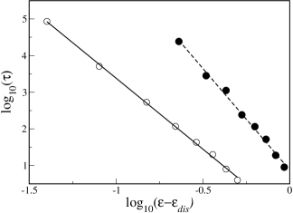
Figure 7: Magnetization relaxation time $\tau$ vs. energy density for two different models. (open symbols) a chain of $N=6$ Heisenberg spins with $R^{-\alpha}$ interaction and $\alpha=2$. A best fit gives $log(\tau)\sim-3.9\ \log(\epsilon-\epsilon_{dis})$, with $\epsilon_{dis}\simeq-0.71$. Here, $\epsilon_{min}=-1.083$. (full symbols) $3$-D cube with an additional spin at the center and nearest neighbor interaction. A best fit gives $log(\tau)\sim-5.5\ \log(\epsilon-\epsilon_{dis})$, with $\epsilon_{dis}\simeq-1.33$. Here, $\epsilon_{min}=-20/9$.

$ii)$ Metastable states. The existence of the TNT has important consequences for the decay time from metastable states. In order to discuss this feature for a simple example, let us consider Hamiltonian (1), adding a term, $B_{y}\sum S_{i}^{y}$, which contains a coupling to an external field directed along the easy–axis of the magnetization. In this case the non–connectivity threshold still exists (it has the same value as before) but the two peaks of $P(m_{y},\epsilon)$ below $\epsilon_{stat}$ do not have the same height, see Fig. 8a. Thus, we can consider the time needed to reach the equilibrium value of the magnetization if we start from a metastable state. Below $\epsilon_{dis}$ metastable states becomes stable for any finite $N$. Above $\epsilon_{dis}$ the decay time diverges at $\epsilon_{dis}$ as a power law, see Fig. 8b. This decay time can be estimated from the statistical properties of the system. Indeed, employing the same simple model described in Sec. (IV.1.1), we can evaluate the decay time scale. Denoting by $P^{+}_{max}$, $P^{-}_{max}$ and $P_{min}$ the probabilities of the thermodynamic stable, metastable and unstable state, respectively (see Fig. 8a), and setting $\lambda_{\pm}=P^{\pm}_{max}/P_{min}$, and $q=P^{+}_{max}/P^{-}_{max}$ we get the following estimate of the decay time:

$$\tau\sim\frac{q}{1+q}\frac{P^{-}_{max}}{P_{min}}.$$ (32)

The good agreement of this estimate with the computed decay times is shown by the crosses in Fig. 8b.

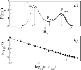
Figure 8: Decay time from a metastable state. In panel $a)$ $P(m_{y})$ is shown for $\epsilon=-0.5$. In panel $b)$ we show the power law divergence of the decay time from a metastable state (full circles). To compute this decay time, $n=100$ initial conditions have been considered for each energy. The best linear fit $log(\tau)=0.309-5.27log(\epsilon-\epsilon_{dis})$ is also shown (dashed line). The decay times computed from Eq. (32) are shown as crosses. Apart from a deviation for high specific energy, the statistically computed decay times are in good agreement with the numerically computed ones (full circles). Parameter values are: $N=6$, $J=3$, $B=0$, $B_{y}=1$

VI Conclusions

Anisotropic Heisenberg spin models with all-to-all coupling show a Topological Non-connectivity Threshold (TNT) energy jsp . Below this threshold the energy surface splits in two components, with opposite easy-axis magnetizations, and ergodicity is broken, even with a finite number $N$ of spins. In the same model, a second order phase transition is present, at an energy higher than the TNT energy. We have fully characterized this phase transition in the microcanonical ensemble, using a newly developed method, based on large deviation theory thierry . For energies in the range between the TNT and the phase transition, magnetization randomly flips if certain strong chaotic motion features are present: the statistics of magnetization reversals is Poissonian. Based on the knowledge of the microcanonical entropy as a function of both energy and magnetization, we have derived a formula for the average magnetic reversal time, which is valid in the large $N$ limit. This formula agrees well with numerical results. The formula also predicts a power law divergence of the mean reversal time at the TNT energy, which is also well verified in numerical experiments. The exponent of the power-law divergence is also in reasonable agreement, although finite $N$ effects are quantitatively important.

Finally, we have shown that all these features (presence of a TNT, power-law divergence of the reversal time, etc.) are not limited to systems with all-to-all coupling. The phenomenology is qualitatively the same for anisotropic Heisenberg spin models with distance dependent interactions and for small clusters of Heisenberg spins with nearest neighbor coupling. We also considered systems where metastable states are present. In this case, while below the TNT they are trapped, above it their decay time diverges as a power law at the TNT. Therefore, we conjecture that the power–law divergence of the magnetic reversal time may be a universal signature of the presence of the TNT, which is a generic feature of systems with long–range interactions or small systems for which the range of the interaction is of the order of system size, if the anisotropy of the coupling is such to determine an easy-axis of the magnetization.

VII Acknowledgments

SR acknowledges financial support under the contract COFIN03 Order and Chaos in Nonlinear Extended Systems. Work at Los Alamos National Laboratory is funded by the US Department of Energy. We thank T. Dauxois, E. Locatelli, F. Levyraz, F. M. Izrailev and R. Trasarti-Battistoni for useful discussions.

Appendix A Minimum energy

In this section we find the minimum of the Mean-Field Hamiltonian (12):

$$\epsilon=m_{z}+\frac{I}{2}(m_{x}^{2}-m_{y}^{2}).$$ (33)

It is sufficient to find the absolute minimum of

$$m_{z}-(I/2)m_{y}^{2},$$

and verify that it satisfies $m_{x}=0$. Taking derivatives

$$\begin{array}[]{lll}\displaystyle\frac{\partial N\epsilon}{\partial\phi_{i}}&=Im_{y}\sin\theta_{i}\cos\phi_{i}=0\\ &\\ \displaystyle\frac{\partial N\epsilon}{\partial\theta_{i}}&=-\sin\theta_{i}-Im_{y}\cos\theta_{i}\sin\phi_{i}=0~{}.\\ \end{array}$$ (34)

one gets two kinds of solutions (both with $m_{x}=0$):

• $\theta_{i}=\pi$ and $\phi_{i}=0,\pi$

• $\phi_{i}=\pm\pi/2$ and $\tan\theta_{i}=\pm Im_{y}.$

Let us define $Nn_{1}$ the number of solutions of type 1) and $Nn_{2}$ the number of solutions of type 2) so that $n_{1}+n_{2}=1$. Since $m_{z}=-n_{1}-n_{2}\cos\bar{\theta}$ and $m_{y}=\pm n_{2}\sin\bar{\theta}$ where $\bar{\theta}$ is the solution of type 2), condition 2) is equivalent to $\cos\bar{\theta}=1/In_{2}$. Therefore, when $In_{2}<1$ the set defined from 2) is empty and only solutions in the class 1) can be obtained. It is also easy to find the expression for the energy in terms of $1/I\leq n_{2}\leq 1$:

$$\epsilon=-1-\frac{1}{2I}+n_{2}-\frac{I}{2}n_{2}^{2}.$$ (35)

Minima must be sought among the extrema so that when $n_{2}=1$ then $e_{min}=-1/2I-I/2$ and when $n_{2}=1/I$ then $\epsilon_{min}=-1$. In terms of $I$, one then has

$$\epsilon_{min}=\left\{\begin{array}[]{lll}&-1/2I-I/2\ {\rm~{}~{}~{}for}\qquad I\geq 1\\ &\\ &-1\quad{\rm~{}~{}~{}~{}~{}~{}~{}~{}for}\qquad I<1.\end{array}\right.$$ (36)

From Eq. (36) we have (10), using transformations in (11).

Appendix B Critical exponents

In this section, we study the divergence of the reversal time for $\epsilon\to\epsilon_{dis}^{+}$, at fixed $N$. Let us assume that it is given by

$$\tau\simeq\max_{m_{y}}P(m_{y},\epsilon)/P(m_{y}=0,\epsilon)~{},$$

we show that

$$\tau\simeq\frac{1}{(\epsilon-\epsilon_{dis})^{\alpha N}}~{},$$ (37)

with $\alpha$ a constant independent of $N$; we find $\alpha=1$ or $\alpha=3/4$, depending on the parameters of the Hamiltonian.

First, we note that although $\max_{m_{y}}P(m_{y},\epsilon)$ increases exponentially with $N$ at fixed $\epsilon$, it does not change much at fixed $N$ when $\epsilon\to\epsilon_{dis}^{+}$; the behavior of $\tau$ is dominated by the value of $P(m_{y}=0,\epsilon)\propto e^{-Ns(m_{y}=0,\epsilon)}$. The problem is then reduced to the computation of $s(m_{y}=0,\epsilon)$.

Before turning to the actual calculation of $s(m_{y}=0,\epsilon\to\epsilon_{dis})$, we consider the following problem, which will be useful later. Let us consider the random variable $x$ in $[-1,1]$ with distribution $\rho(x)$; we call $m=\sum_{i=1}^{N}x_{i}/N$, and ask the question: what is the behavior of $P(m=1-\delta),~{}\delta<<1$, for fixed $N$ reasonably large? Using Cramér’s theorem, we write

$$\Psi(\lambda)=\int_{-1}^{1}\rho(x)\exp(\lambda x)dx$$ (38)

and

$$s(m)=-\sup_{\lambda}\left(\lambda m-\ln\Psi(\lambda)\right)~{}.$$ (39)

$m\to 1$ implies $\lambda\to\infty$, so the behavior of $\rho$ close to $x=1$ dominates (38). We write $\rho(x)\sim a(1-x)^{\gamma}$, close to $x=1$, with $\gamma>-1$. Then for $\lambda\to\infty$,

$$\Psi(\lambda)\sim a\frac{e^{\lambda}}{\lambda^{\gamma+1}}\int_{0}^{\infty}u^{\gamma}e^{-u}du~{}.$$

Then the maximizing $\lambda$ in (39) is given by $m=1-(\gamma+1)/\lambda$. Substituting into (39), we get $s(m=1-\delta)\sim(\gamma+1)\ln\delta$, and finally, $P(m=1-\delta)\sim\delta^{N(\gamma+1)}$.

We now apply this result to the easiest case, the simplified Hamiltonian $H=N(m_{z}+I(m_{x}^{2}-m_{y}^{2})/2)$. The threshold is $\epsilon_{dis}=-1$ (we consider the case $I>1$); we write $\epsilon=-1+\delta$, with $\delta<<1$. We want to compute the entropy $s(m_{x},m_{y}=0,m_{z}=-1+\delta-Im_{x}^{2})$. Noticing that a small $\delta$ implies a small $m_{x}$, we simplify the calculation to $s(m_{x}=0,m_{y}=0,m_{z}=-1+\delta)$. We now use once again Cramér’s theorem.

$$\Psi(\lambda_{x},\lambda_{y},\lambda_{z}) = \frac{1}{4\pi}\int_{0}^{\pi}~{}\sin\theta d\theta\int_{0}^{2\pi}d\phi\exp(\lambda_{x}\sin\theta\cos\phi)$$ (40)

$$\exp(\lambda_{y}\sin\theta\sin\phi+\lambda_{z}\cos\theta)~{}.$$

Then $s$ is given by:

$$s(m_{x},m_{y},m_{z}) = -\sup_{\lambda_{x},\lambda_{y},\lambda_{z}}\left[m_{x}\lambda_{x}+m_{y}\lambda_{y}+m_{z}\lambda_{z}\right.$$ (41)

$$\left.-\ln\Psi(\lambda_{x},\lambda_{y},\lambda_{z})\right]~{}.$$

For $m_{x}=m_{y}=0$, the maximizing $\lambda_{x}$ and $\lambda_{y}$ are found to vanish. Thus, the problem reduces to calculating $s(m_{z}=1-\delta)$ (using also the symmetry $m_{z}\to-m_{z}$). Recalling that $m_{z}=\langle\cos\theta\rangle$, with $\theta$ the latitude of a point taken randomly on the sphere with uniform probability. This is equivalent to saying that $m_{z}=\langle q\rangle$, with $q$ a random variable uniformly distributed between $-1$ and $1$. Using the general result derived above with $\gamma=0$, we find that $\tau\sim(\epsilon-\epsilon_{dis})^{\alpha N}$, with $\alpha=1$.

We turn now to the complete Hamiltonian, with $B=0$, $H=N(I(m_{x}^{2}-m_{y}^{2})/2-J\Delta/2)$. The threshold is now $\epsilon_{dis}=-J/2$. We set $\epsilon=-J/2~{}(1-\delta)$. Noticing that again, a small $\delta$ implies a small $m_{x}$, we compute $s(m_{x}=0,m_{y}=0,\Delta=1-\delta)$, in the limit of small $\delta$. $\Delta$ is defined as $\langle\sin^{2}\theta\cos 2\phi\rangle$, for $\theta$ and $\phi$ coordinates of points taken randomly on the sphere with uniform probability. Again, this is equivalent to saying that $\Delta=\langle q\rangle$, with $q$ now having a non uniform distribution $\rho(q)$ in $[-1,1]$. However, $\rho(q)$ tends to a constant value as $q\to 1^{-}$ (the calculation is detailed at the end of the appendix), which means $\gamma=0$; thus Eq.(37) holds, again with $\alpha=1$. The conclusion is the same for all $B\neq J$.

Finally, we consider now the case $B=J=1$. Then $H=N(m_{z}+N(m_{x}^{2}-m_{y}^{2})/2-\Delta/2)$. Setting $\epsilon=-(1-\delta)$, we want to compute $s(m_{x}=0,m_{y}=0,m_{z}-\Delta/2=1-\delta)$. Calling $M=m_{z}-\Delta/2$, we have $M=\langle q\rangle$, with $q=\cos\theta-(\sin^{2}\theta\cos 2\phi)/2$ a random variable in $[-1,1]$ with distribution $\rho(q)$. The calculations in the next paragraph show that $\rho(q)$ diverges at the boundary like $(1-q)^{\gamma}$, with $\gamma=-1/4$; thus Eq.(37) still holds, now with $\alpha=3/4$.

Derivation of the exponent $\gamma$ :

1. $\mathbf{B=0}$: we need to compute the distribution $P(y=\sin^{2}\theta\cos 2\phi)$, close to $y=1$. We have, with $u=\cos\theta$:

$$P(y)=\int_{-1}^{1}du\int_{0}^{2\pi}d\phi~{}\delta_{D}\left(y-(1-u^{2})\cos 2\phi\right)~{},$$ (42)

where $\delta_{D}(x)$ is the Dirac delta function. Writing $y=1-\delta$, with $\delta\ll 1$, we see that only the values of $u$ such that $u^{2}<\delta$ contribute. Integrating over $\phi$ we obtain:

$$P(1-\delta)=4\int_{-\sqrt{\delta}}^{\sqrt{\delta}}\frac{du}{2((1-u^{2})^{2}-(1-\delta)^{2})^{1/2}}~{};$$ (43)

the factor of $4$ in front comes from the four values of $\phi$ that contribute the same amount to $P$. Expanding the denominator, neglecting order $\delta^{2}$ terms and performing the change of variable $u=\sqrt{\delta}t$, we get:

$$P(1-\delta)\simeq\int_{-1}^{1}\frac{\sqrt{2}dt}{\sqrt{1-t^{2}}}~{}.$$ (44)

Since this last integral does not depend on $\delta$ and has a finite value, we conclude that $\gamma=0$ for $B=0$.

2. $\mathbf{B=J=1}$: we need to compute now $P(y=u-(1/2)(1-u^{2})\cos 2\phi)$ close to $y=1$. This reads:

$$P(y)=\int_{-1}^{1}du\int_{0}^{2\pi}d\phi\delta_{D}\left(y-u+\frac{1}{2}(1-u^{2})\cos 2\phi\right)~{}.$$ (45)

Solving for $\phi$ inside the delta function, we get

$$\cos 2\phi=\frac{2(u-y)}{1-u^{2}}~{}.$$ (46)

This time, only the values of $u$ close to $u=1$ contribute to $P$; thus, we write $u=1-s$, $y=1-\delta$. From the inequalities $-1\leq\cos 2\phi\leq 1$, we get, neglecting terms of order $s^{2}$, $\delta/2\leq s\leq\sqrt{2\delta}$. Integrating the delta function over $\phi$, we have the expression for $P$:

$$P(1-\delta)\simeq 4\int_{\delta/2}^{\sqrt{2\delta}}\frac{ds}{\left((2s-s^{2})^{2}-4(\delta-s)^{2}\right)^{1/2}}~{};$$ (47)

the change of variable $t=2s/\delta$ yields

$$P(1-\delta)\simeq\int_{1}^{\sqrt{8/\delta}}\frac{dt}{\sqrt{t-1}}~{}.$$ (48)

This integral converges close to $t=1$; it diverges however at large $t$, like $t^{1/2}$; since $t$ diverges as $\delta^{-1/2}$, we finally get $\gamma=-1/4$.

3. General case $\mathbf{B\neq J}$: we do not detail here the calculations, which are similar to those above. As soon as $B\neq J$, the result is $\gamma=0$, and thus $\alpha=1$.

References

- (1) D. H. E. Gross Microcanonical Thermodynamics: Phase Transitions in Small Systems, Lecture Notes in Physics 66, World Scientific, Singapore, 2001.
- (2) F. Borgonovi, G. Celardo, F. M. Izrailev, and G. Casati Phys. Rev. Lett., 88, 054101 (2002); V. V. Flambaum and F. M. Izrailev, Phys. Rev. E, 56, 5144, (1997); F. Borgonovi and F. M. Izrailev, Phys. Rev. E, 62, 6475 (2000); F. Borgonovi, I. Guarneri, F. M. Izrailev and G. Casati, Phys. Lett. A, 247, 140 (1998).
- (3) M. Hartmann, G. Mahler and O. Hess. Phys. Rev. Lett. 93, 80402 (2004).
- (4) F. Borgonovi, G. L. Celardo, M. Maianti, E. Pedersoli, J. Stat. Phys., 116, 1435 (2004).
- (5) F. Borgonovi, G. L. Celardo, A. Musesti, R. Trasarti-Battistoni and P. Vachal, cond-mat/0505209.
- (6) L. Q. English, M. Sato and A. J. Sievers, Phys. Rev. B , 67, 24403 (2003); M. Sato et al., Jour. of Appl. Phys., 91 , 8676 (2002).
- (7) T. Dauxois, S. Ruffo, E. Arimondo, M. Wilkens Eds., Lect. Notes in Phys., 602, Springer (2002).
- (8) R. S. Ellis, Physica D, 133, 106 (1999); J. Barré, F. Bouchet, T. Dauxois, S. Ruffo, J. Stat. Phys. 119, 677 (2005); J. Barré, Phd Thesis, ENS-Lyon, (2003).
- (9) We simulated the dynamic of the system through a Runge Kutta -th order integrator.
- (10) G. L. Celardo, PhD Thesis, Univ. of Milan (2004).
- (11) For the results for odd and even coincide up to () corrections.
- (12) E. M. Chudnovsky and J. Tejada, Macroscopic Quantum Tunneling of the Magnetic Moment, Cambridge University Press, (1998).
- (13) A. Dembo, O. Zeitouni, Large Deviations Techniques and Applications, (Springer, Berlin, 1998).
- (14) Note that the same distribution can be obtained, in a fully chaotic regime, from the time series of .
- (15) Sh. Kogan, Electron Noise and Fluctuations in Solids Cambridge Univ. Press., Cambridge (1996).
- (16) M. Antoni, S. Ruffo and A. Torcini, Europhys. Lett., 66, 645 (2004).
- (17) P. H. Chavanis and M. Rieutord Astronomy and Astrophysics, 412, 1 (2003); P. H. Chavanis, astro-ph/0404251.
- (18) L. D. Landau and E. M. Lifshitz, Statistical Physics Pergamon Press, Oxford (1985).
- (19) R. B. Griffiths, C. Y. Weng, and J. S. Langer, Phys. Rev., 149, 1 (1966).
- (20) M. Kac, G. E. Uhlenbeck and P. C. Hemmer, J. Math. Phys., 4, 216 (1963).
- (21) B.V.Chirikov Phys. Rep., 52, 253 (1979).