Abstract

In this study, the additional heat capacity which appear during the water dissociation of the proteins that are one of the soft materials, have been considered by the statistical mechanical methods. For this purpose, taking the electric field E and total dipole moment M as the thermodynamical variables and starting with the first law of thermodynamics an equation which reveals the thermodynamical relation between the additional heat capacity in effective electric field $\triangle C_{E}$ and the additional heat capacity at the constant total dipole moment $\triangle C_{M}$, has been obtained. It is found that, the difference between the heat capacities depends linearly on the temperature. To bring up the hydration effect during the folding and unfolding of the proteins the physical properties of the apolar dissociation have been used. In the model used for this purpose; the folding and unfolding of the proteins in the formed electric field medium have been established on this basis. In this study with the purpose of revealing the additional effect to the heat capacity, the partition functions for the proteins which have been calculated in single protein molecule approach by A. Bakk, J.S. Hoye and A. Hansen; Physica A, 304, (2002), 355-361 have been taken in order to obtain the free energy. In this way, the additional free energy has been related to the heat capacities. By calculating the heat capacity in the effective electric field $\triangle C_{E}$ theoretically and taking the heat capacity at constant total dipole moment $\triangle C_{M}$ from the experimental data, the outcomes of the performed calculations have been investigated for Myoglobin and other proteins.

Keywords: Thermodynamics, Classical statistical mechanics

PACS 05.70-a, 05.20-y

^∗ Corresponding Authors:e-mail:oylum@sci.ege.edu.tr, Phone:+90 232-3881892 (ext.2363) Fax:+90 232-3881892

^∗∗ e-mail:fevzi@sci.ege.edu.tr, Phone:+90 232-3881892 (ext.2846)
^∗∗∗ e-mail:dogan@sci.ege.edu.tr, Phone:+90 232-3881892 (ext.2381)

1 Introduction

Now a days, a progress in the direction of investigation of the soft materials by the methods of statistical physics is realized. It is not possible to think a way of life without the soft materials; all biological structures, the molecules of the genetic code, proteins and membranes contain soft materials. Soft materials are the fundamentals of the life and an important component of the future technological developments.

Proteins is a common name for the complex macromolecules which are formed by unification of a great number of amino-acids and which play unabandonable roles in the life times of all the living creatures. When considering the physical problem of formation of the structure of the natural proteins, one must keep in mind that proteins are quite different molecular objects. As a physical object the protein molecule is rather a big polymer composed of thousands of atoms and is such a soft material that from the physical point of view it is a macroscopic system.

Every single atom forming the proteins occupies a place at a certain position as in the crystals. However, unlike to the crystals the position of each atom is unique to itself with respect to the neighboring atoms. Consequently, proteins represent a macroscopic system which is different from the crystals such that here the order is not periodical. A protein could be synthesized as a linear heterogeneous polymer which is formed by a genetically determined order where the remainders of different amino-acids are bounded to each other by peptide bounds. This polypeptide chain folds to a self unique conformation which is completely determined by the information in the ordering of the remainders of the amino-acids. The folding of the polypeptide chain to a three dimensional structure, principally is a reversible process and this depends on environmental conditions. In other words, thermodynamically, this process is passing from an unfolded state to another rather ordered macroscopic state. This case is named as the natural state of the protein molecule.

2 Model

For different aspects of the folding and unfolding transitions of the proteins various models have been proposed [1, 2]. Simple but yet a notable model among then is the zipper model which defines the helix chain. In another model, the idea of representing the solvent as dipoles in the unfolding of proteins was given by the work of Warshel and Levitt and later on in the applications of Rushell, Fan and Avbelj [3, 4]. In order to model the effect of the folding of the proteins Bakk asked for the inclusion of important physical properties in apolar dissolution. For this purpose he started by choosing the water molecules as classical dipoles [5].

2.1 First Law of the Thermodynamics for the Proteins

By taking the electric field E and the total dipole moment M as thermodynamical variables the first law of thermodynamics could be written for the proteins:

$$dU=TdS-MdE.$$ (1)

Here, the electric field is not an external field but is used to model the ice-like behavior of the water molecules around non-polar surfaces. The electric field is a result of the effective behavior of the non-polar solvent applied in the unfolding of the protein. By considering the proteins as soft materials, the thermodynamical relation between the heat capacity at effective electric field $\triangle C_{E}$ and the heat capacity at constant total dipole moment $\triangle C_{M}$ has been put forward. Re-arranging Eq.(1) one could write

$$dQ=dU+MdE.$$ (2)

To constitute such a relation, first of all the internal energy U is written as the total differential of the variables T and E and then substituted in Eq.(2) giving

$$dQ=(\frac{\partial U}{\partial T})_{E}dT+[M+(\frac{\partial U}{\partial E})_{T}]dE.$$ (3)

When the relevant heat capacities for constant M and E are written down in Eq. (3) one obtains:

$$\triangle C_{M}=\triangle C_{E}+[M+(\frac{\partial U}{\partial E})_{T}](\frac{\partial E}{\partial T})_{M}$$ (4)

with the aim of expressing the term in the right hand side of Eq.(4) in terms of experimentally measurable quantities, Eq.(4) has been written in a different form, the total differentials of U(T,E) and S(T,E) have been calculated, the partial differentiations on both sides of equation have been performed and as a result the following expression has been found

$$\triangle C_{M}=\triangle C_{E}+T(\frac{\partial M}{\partial T})_{E}(\frac{\partial E}{\partial T})_{M}.$$ (5)

Now, using properties of the total differential and also Maxwell relations constituted for the proteins

$$\triangle C_{M}-\triangle C_{E}=-T(\frac{\partial M}{\partial E})_{T}[(\frac{\partial E}{\partial T})_{M}]^{2}$$ (6)

has been obtained.

Eq.(6) reveals the thermodynamical relation between the heat capacity at effective electric field $\triangle C_{E}$ and the heat capacity at constant total dipole moment $\triangle C_{M}$. It is seen in the equation that; the difference of the heat capacities depend linearly on the temperature. $\triangle C_{E}$ in Eq.(6) could easily be calculated theoretically and if $\triangle C_{M}$ is measured experimentally, one could get a means of investigating the system in terms of thermodynamical quantities.

2.2 Single Protein Approach

Let us suppose that each atom has a dipole moment $\overrightarrow{p}$ and interatomic interactions could be neglected. In the absence of an electric field each of the molecules has a continuous and randomly oriented dipole moment.

On the non-denatured protein surface, in the positive bound charges (ions) of the water molecules an ice-like construction by the solvent effect becomes a matter of question. This in turn leads to the orientation of the dipole moments of the polar water molecules in the direction of field as if an external field were applied on the water molecules. This rigidness is for providing the water molecules to stay around the apolar surfaces. Thus this is not a real external field but reflects the characteristics of the solvation of the water molecules around the positive ions the non-polar surface in the protein folding.

In this case the force on each dipole solely originates from the produced electric field. Since each atom experiences thermal agitation, the energy distributions of these atoms could be investigated by Classical Maxwell-Boltzmann Statistics [6]. The number of atoms $dN$ in the energy internal $U$ and $U+dU$ is written as;

$$dN=C\exp(-U\beta)dU$$ (7)

where $\beta=1/kT$, k is the Boltzmann constant, T is the absolute temperature and C is a constant. $U$ being the energy of the proteins, the energy gained by the dipole due to the applied field is given by

$$U=-\overrightarrow{p}\cdot\overrightarrow{E}.$$ (8)

Let the angle between the axis of the dipole and the electric field be $\theta$, then change in the amount of the electrical potential energy that the dipole possessed is obtained as

$$dU=pE\sin\theta d\theta.$$ (9)

When $dU$ is substituted in Eq.(7), the number of atoms in the energy interval $U$ and $U+dU$ could be obtained in the following form

$$dU=C\exp(pE\beta\cos\theta)pE\sin\theta d\theta.$$ (10)

If total number of atoms per unit volume is defined as $N=\int^{\pi}_{0}dN$, then one writes for the total dipole moments as

$$M=N<m>=\int^{\pi}_{0}m\cos\theta dN$$ (11)

where $<m>=\overline{m}$ which is the average dipole moment per atom in the direction of the formed electric field. When the equation expressing the total number of atoms is substituted in Eq.(11) the solution in terms of the Langevin function is found as

$$M=mL(a)$$ (12)

where $pE\beta=a$.

2.3 Hydration Effect to the Single Protein Approach

In addition to the energy coming from the external field, in order to introduce the pair interactions to the model pairing term must be added. For the purpose of obtaining an effective field in $U_{e}$ if two equations written initially are combined for a water molecule the effective field for this case becomes [4, 5]

$$U_{e}=U_{DPE}+U_{MF}.$$ (13)

Substituting the mean-field solution of the hydration effect in the single protein approximation, one obtains for the dipole moment [4, 7]

$$m=\int^{2\pi}_{0}d\phi\int^{\pi}_{0}d\theta\cos\theta\sin\theta\exp(-\beta U_{e}).$$ (14)

Supposing that, distribution of the electric dipole moments has canonical distribution forms and making use of the fact that the orientations of p vectors stay in the intervals $\theta+d\theta$ and $\phi+d\phi$, from the definition of the solid angle $d\Omega=\sin\theta d\theta d\phi$, one gets the partition function for a protein as

$$z=\int\int\exp(-\beta U_{e})d\Omega.$$ (15)

When solid angle $d\Omega$ and the explicit expression for $U_{e}$ are substituted in the integral, one gets

$$z(T,E,N=1)=4\pi\exp^{-\frac{\beta bm^{2}}{2}}\frac{1}{\beta\epsilon_{e}}{\sinh\beta\epsilon_{e}}.$$ (16)

By making use of the definition for the average dipole moment $<m>=m/z$; it is obtained in the form $<m>=L(\beta\epsilon_{e})$. Here the effective energy is given by $\epsilon_{e}=\epsilon+b<m>$. The partition function of the system is the multiplication of N number of single particle partition functions.

In thermodynamical investigation of the protein system, in order to introduce the chemical potential $\mu$ (here takes the place of pH), one has to take the system in a macro-canonical ensemble. In this study, the macro-canonical ensemble is obtained from the canonical ensemble. Here in addition to be heat bath, it is supposed that the system is in a particle reservoir and if this reservoir is large, in the equilibrium, the particles reach an average value.

In the first approximation, if the expression found in Eq.(16) for the canonical ensemble is extended for the macro-canonical case, without putting any limit on the particle number [6] one could use the relation

$$Z(T,E,\mu)=\sum^{\infty}_{N=0}\frac{1}{N!}[\exp(\frac{\mu}{kT})z(T,E,N=1)]^{N}.$$ (17)

The partition function of the undistinguishable particles which is given by Eq.(17) is obtained as

$$Z(T,E,\mu)=\exp[\exp(\frac{\mu}{kT})z(T,E,N=1)]$$ (18)

where the expression $\zeta=\exp(\beta\mu)$ corresponds to the pH of the system and is the weight factor. In this case,

$$<U>=-\frac{1}{Z}\frac{\partial}{\partial\beta}(Z)_{\zeta},_{E}$$ (19)

is written for the energy of the system. Here, the expression $\Phi(T,E,\mu)=-\frac{\ln Z(T,E,\mu)}{\beta}$ is the thermodynamical potential. After the partition function obtained by the substitution of Eq.(16) in Eq.(18) the thermodynamical quantities of the system are found as follows:

Entropy is given by the formula

$$S(T,E,\mu)=-(\frac{\partial\Phi}{\partial T})_{E},_{\mu}$$

which then leads to

$$S(T,E,\mu)=k[\ln[\exp(\frac{4\exp\beta(\mu-\frac{bm^{2}}{2})}{\epsilon_{e}\beta})]$$

$$+\frac{\exp\beta(\mu-\frac{bm^{2}}{2})[-4\pi\epsilon_{e}\beta\cosh(\epsilon_{e}\beta)}{\beta\epsilon_{e}}+$$

$$\frac{2\pi(2+\beta bm^{2})\sinh(\epsilon_{e}\beta)]}{\beta\epsilon_{e}}]$$

total dipole moment is given by the formula

$$M(T,E,\mu)=-(\frac{\partial\Phi}{\partial E})_{T},_{\mu}$$ (20)

which then leads to

$$M(T,E,\mu)=\frac{4\pi\exp(\beta(\mu-\frac{bm^{2}}{2}))}{\epsilon_{e}^{2}\beta^{2}}$$

$$(\epsilon_{e}\beta\cosh(\epsilon_{e}\beta)-\sinh(\epsilon_{e}\beta))$$

and lastly the particle number is given by the formula

$$N(T,E,\mu)=-(\frac{\partial\Phi}{\partial\mu})_{T},_{E}$$ (21)

leading to

$$N(T,E,\mu)=\frac{4\exp(\beta(\mu-\frac{bm^{2}}{2}))\pi\sinh(\epsilon_{e}\beta)}{\epsilon_{e}\beta}.$$

3 Variation of the Additional Heat Capacity with Temperature

In this study the variation of $\triangle C_{M}$ with temperature has been investigated. In the macro-canonical ensemble the additional heat capacity in the effective electric field for the protein system is calculated from the expression

$$\triangle C_{E}=(\frac{\partial U}{\partial T})_{\zeta},_{E}-\frac{1}{T}(\frac{\partial N}{\partial\mu})_{E},_{T}[(\frac{\partial U}{\partial N})_{T},_{E}]^{2}.$$ (22)

On the other hand, the variation of the internal energy with temperature is given by

$$(\frac{\partial U}{\partial T})_{\zeta},_{E}=(\frac{\partial U}{\partial T})_{E},_{N}+(\frac{\partial U}{\partial N})_{T},_{E}(\frac{\partial N}{\partial T})_{\zeta},_{E}.$$ (23)

For $(\frac{dU}{dN})_{T,E}$ in Eq.(23)

$$(\frac{\partial U}{\partial N})_{T},_{E}=\frac{(\frac{\partial U}{\partial T})_{\zeta},_{E}-(\frac{\partial U}{\partial T})_{E},_{N}}{(\frac{\partial N}{\partial T})_{\zeta},_{E}}$$ (24)

is substituted which is attained from Eq.(24).

$\triangle C_{E}$ is substituted in Eq.(6). $M,S$ and $N$ that are necessary in Eq.(6) and Eq.(25) have been taken from Eq.(21), Eq.(20) and Eq.(22) respectively. The explicit forms of the above expressions are lengthy and thus are not written down.

In order to compare $\triangle C_{M}$ which is found theoretically with the experimental values of $\triangle C_{M}$ they are shown on the same plot in Fig(1). The dashed curves represent the experimental study and the solid curves represent the theoretical result. In this semi-phenomenological theory, the physical quantities $\epsilon$ , $b$ and $\mu$ curves have been determined by fitting to the results of Privalov and Bakk .

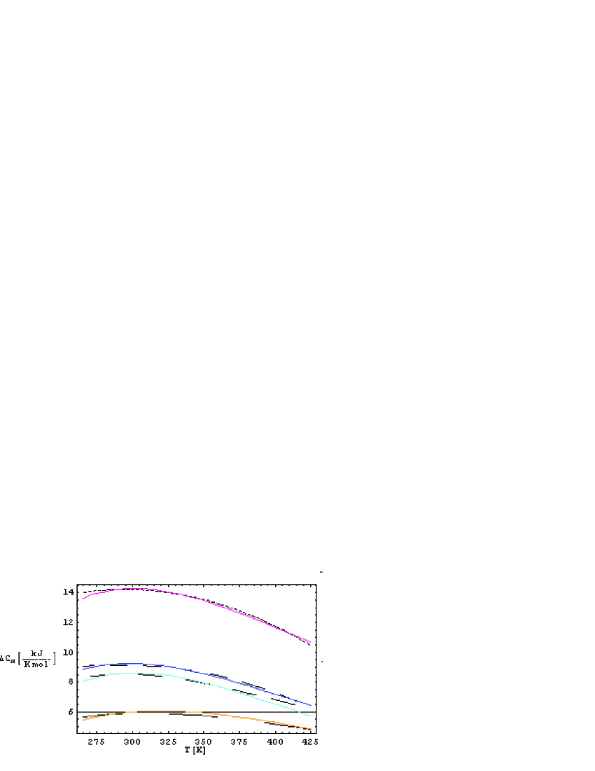
Figure 1: Graph of the variation of the additional heat capacities with temperature.

Red (Myoglobin), blue (Lysozyme), green (Cytochrome) and Yellow (Ribonuclease) solid curves represent the variation of the additional heat capacity difference with temperature obtained from theoretical result.

Table 1: Additional heat capacity values corresponding to transition temperature for four different proteins.

Color	Protein	AHCD$(\frac{kJ}{Kmol})$	Trans. Temp.$(K)$
Red	Myoglobin	14.3	301
Blue	Lysozyme	9.3	298
Green	Cytochrome	8.6	302
Yellow	Ribonuclease	6.1	320

A H C D :  Additional Heat Capacity Differences

4 Conclusions

In this study a theory of the heat capacity depending on electrostatic field and constant dipole moment in the transition between the fold and unfold states of the protein molecule according to Bakk [4] model, has been presented. The foresight of the performed calculations have been discussed by taking into account the experimental studies of Privalov and Makhatadze on Myoglobin, Lysozyme, Cytochrome and Ribonuclease in the interval $275-350K$ [8, 9].

Biological and other macromolecular systems exhibit great variations in heat capacity with respect to temperature. The unfolding of the globular proteins in water is a classical example. Change in the environmental conditions such as temperature, increase or decrease in pH, interaction of the solution dissolvers with protein molecule groups, gives rise to the change in the structure of the proteins.

When the conditions return to their initial state these molecules return to their former structures. The folding and then unfolding of these molecules occur by a thermodynamical mechanism. When the graph of the variation of the additional heat capacities with temperature is examined one could state that the behavior of the proteins exhibits approximately an universal behavior. The apex in the heat capacity curve indicates the denaturation transition. For each of the four proteins; additional heat capacity difference and transition temperatures $T_{t}$ correspond to different values and the numerical values have been presented in Table 1. For every protein in native state the heat capacity is less than the value in the denature field. The transition between the native and denature state is a first order transition.

An additional reason of the observed increase in the heat capacity is the hydration effect. The transformation of the apolar solvents into water, takes place with a considerable increase in the heat capacity. A conclusion drawn here is that; depending on the unfolding of the proteins, the additional increase in the heat capacity is a consequence of the contact of the internal groups during the unfolding of the proteins. The hydration effect originates from the low solubility of the apolar compounds in water.

One of the characteristics of the folding and unfolding of the proteins is that, the temperature interval of the process depends on environmental conditions and particularly on the pH values of the solution. This task is supplied by the term $\zeta=\exp(\beta\mu)$ in the partition function. Variations in the enthalpy difference relevant to pH will be presented in a forthcoming article.

5 Acknowledgment

One of the authors, G.O. thanks to Prof. Dr. Sener Oktik, rector of the Mugla University for his contributions as well as his support to stay in Ege University, Physics Department where this study has been carried out.

References

- [1] A. Hensen, H. Jensen, K. Sneppen and G. Zocchi, EPJ B6, (1998) 157-161.
- [2] A. Hensen, H. Jensen, K. Sneppen and G. Zocchi, Pyhsica A 270, (1999) 278-287.
- [3] H.S. Frank and M.W. Evans, J. Chem. Phys. 13, (1945) 507-532.
- [4] A. Bakk, J.S. Hoye and A. Hansen, Pyhsica A 304, (2002) 355-361
- [5] B. Madan and K. Sharp, J. Phys. Chem. B 101, (1997) 11237-11242.
- [6] W. Greiner, L. Neise and H. St cher, Thermodynamics and Statistical Mechanics (Springer-Verlag, 1995) 246-253
- [7] P. Bruscolini, xxx.lanl.gov cond-mat 0305288v1.
- [8] P.L. Privalov, J. Chem. Thermodynamics 29, (1997) 447-474.
- [9] T.E. Creighton, Protein Folding (W.H. Freeman And Company New York, 1995) 83-151