A few bubbles in a glass

Abstract

I briefly review a recent series of papers putting forward a coarse-grained theoretical approach to the physics of supercooled liquids approaching their glass transition. After a suitable coarse-graining, the dynamics of the liquid is replaced by that of a mobility field, which can then be analytically treated. The statistical properties of the mobility field then determine those of the liquid. Thermodynamic, spatial, topographic, dynamic properties of the liquid can then be quantitatively described within a single framework, and derive from the existence of an underlying dynamic critical point located at zero-temperature, where timescales and lengthscales diverge.

I Why do glasses exist?

One of the peculiarities of the field of glass transition phenomena is that the object of study itself was already known to mankind thousands of years ago. Therefore, obtaining the material to be studied is straightforward, and Nature itself produces abundant quantities of amorphous solids review1 ; review2 ; review3 . The point is rather to understand why glasses exist. What is the microscopic mechanism that produces glassy materials? Does a glass state truly exist? Can one describe the glass formation in theoretical terms similar to the ones used for other cooperative phenomena, such as continuous phase transitions?

Experiments performed on liquids supercooled through their melting transition towards the glass transition have characterized static and dynamic aspects in much detail, so that a number of “canonical features” associated to the formation of glasses are well-known review3 : broad relaxation patterns, extremely fast increase of relaxation times when temperature is decreased, non-conventional hydrodynamics, dynamic heterogeneity, all phenomena being accompanied by no drastic change in the structure of the material that simply resembles that of a normal liquid.

In a recent series of paper p1 ; p2 ; p25 ; p3 ; p4 ; p6 ; p5 ; p8 ; p9 ; p7 ; p30 ; fss , it was shown that all these phenomena can be explained within a relatively simple and unique framework after a suitable coarse-graining mapping the density field to a mobility field. After coarse-graining, the system becomes simple enough that the statistical properties of the mobility field can be worked out in an essentially non-mean-field manner, yielding analytical results and a set of quantitative predictions. The physics is qualitatively explained in terms of non-trivial spatio-temporal correlations of the mobility field, that have been called bubbles. Analytical results suggest that these fluctuations are critical in the sense that they reflect the presence of a zero-temperature dynamic critical point where lengthscales and timescales diverge, which was therefore proposed to be responsible for the experimentally observed glass transition.

The paper is organized as follows. We first explain how the dynamics of supercooled liquids is mapped onto a mobility field exhibiting non-trivial spatio-temporal correlations. We then show that the presence of these dynamic bubbles is sufficient to qualitatively explain the physics. We finally show that bubbles are the direct manifestation of dynamic critical fluctuations that can be analyzed through the renormalization group.

II From molecules to bubbles

II.1 Coarse-graining

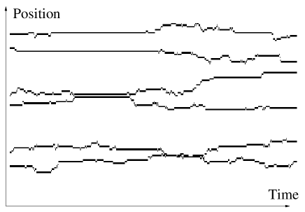
Figure 1: A piece of trajectory of six randomly chosen probe molecules in one of the coarse-grained models discussed in this paper. Molecules are caged for long periods of time (horizontal lines) before hopping and becoming trapped again. Note that two molecules coming sufficiently close to one another have correlated dynamics. At a given time step, some molecules are hopping while others are trapped, and the system is therefore dynamically heterogeneous.

Traditionally, simple liquids are described in terms of the density field,

$$\rho(x,t)=\sum_{i=1}^{N}\delta\big{(}x-x_{i}(t)\big{)},$$ (1)

where $x_{i}(t)$ is the position of particle $i\in\{1,\cdots,N\}$ at time $t$. This is because the structure of the liquid can be expressed in terms of various density correlators, whose analytical treatment can be found in classic textbooks jl . When the temperature of a supercooled liquid is decreased towards the glass temperature, the static structure barely evolves despite dramatic changes in the particles’ dynamics, indicating that standard liquid theory might be of modest utility here.

An amorphous solid is obtained when the diffusion constant of the particles becomes unmeasurably small. Above the glass transition, however, diffusion holds at sufficiently large time and length scales. A closer inspection of the particles’ trajectories reveals the specificities of supercooled liquids, see Fig. 1. On timescales of the order of the relaxation time, $\tau_{\alpha}$, trajectories do not resemble a classic random walk. Rather, particles are immobile for long periods of time, before diffusing and eventually being stuck again. In the traditional jargon, particles are “caged”, or “trapped”, before “hopping”. This leads to a two-step decay of dynamic correlators, corresponding to a fast “rattling” of the particles within their cages, and a much slower decay corresponding to the “structural” decay of the liquid associated to hopping. Explaining this two-step decay, and elucidating the properties of both processes is the main theoretical task in the field.

The main idea of the approach described in this paper is to map the density field, $\rho(x,t)$, to a mobility field, $\varphi(x,t)$. The mapping is illustrated in Fig. 2, where the trajectories of Fig. 1 are superposed to the dynamics of a binary mobility field, $\varphi(x,t)=0,1$. A particle immersed in a sea of immobility (white) does not move, it is caged. A particle can move when sitting on a mobile region, or “defect” (black). It turns out that the dynamics of $\varphi(x,t)$ can be empirically determined, leading to well-defined, solvable models from which predictions can be made. The obtained theory does not start from first-principles, but it allows one to address analytically all desired aspects of the physics. Comparison to experiments or simulations provides then the necessary check of the correctness of the approach.

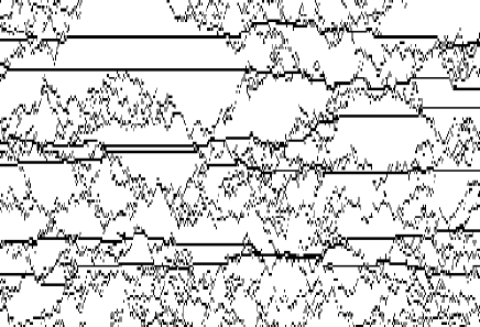
Figure 2: From molecules to bubbles. The molecular trajectories of Fig. 1 are superposed with the trajectory of an underlying binary mobility field. Black denotes mobile regions, $\varphi=1$, white immobile ones, $\varphi=0$.

Schematically, the mobility field can be obtained via a temporal and spatial coarse-graining p1 ,

$$\varphi(x,t)=1-\frac{1}{V_{x}}\int_{V_{x}}d^{d}x^{\prime}\left(\frac{\rho(x^{\prime},t)\rho(x^{\prime},t+\delta t)-\langle\rho\rangle^{2}}{\langle\rho^{2}\rangle-\langle\rho\rangle^{2}}\right),$$ (2)

so that $\varphi(x,t)\approx 0$ if the local mobility is low, $\varphi(x,t)\approx 1$, otherwise. The coarse-graining procedure makes use of a volume $V_{x}\sim\xi_{\rm s}^{d}$ centered in $x$, where $d$ is the space dimensionality, and $\xi_{\rm s}$ is the static correlation length as given by the structure factor, and a microscopic time scale, $\delta t$, of the order of ps. Doing so, we lose track of the fast vibrational properties of the liquid, which are thought to be irrelevant for the glass transition problem. In that sense, the approach is close in spirit to inherent structure studies where real trajectories are mapped onto local minima of the potential energy surface, also removing fast vibrations, see Refs. still ; is1 ; is2 .

Note finally that more complex, e.g. vectorial, mobility field can be defined, in order to capture a possible local anisotropy of the dynamic facilitation east . Persistence or absence of directionality of the dynamic constraint can be shown to lead to fragile and strong behaviours, as analyzed in detail in Ref. p1 .

II.2 Link with kinetically constrained models

After coarse-graining, Eq. (2), the properties of the mobility field $\varphi(x,t)$ remain to be described. Here, two phenomenological assumptions are made.

(i) Since dynamics at low temperature is very slow, it is natural to expect that $\langle\varphi(x,t)\rangle\ll 1$ at low temperatures. Therefore, the simplest choice is to assume that mobile regions are so sparse that they do not interact. Thermodynamics is then assumed to be that of a non-interacting gas of point defects of mobility.

(ii) The time evolution of $\varphi(x,t)$ makes use of the concept of dynamic facilitation, introduced long ago fa ; prl . It is assumed that a region can evolve, and therefore satisfy $\partial_{t}\varphi\neq 0$, if and only if surrounded by regions of high mobility. The simplest rule is to assume that

$$\frac{\partial\varphi(x,t)}{\partial t}\propto\int_{\partial V_{x}}d^{d}x^{\prime}\,\varphi(x^{\prime},t),$$ (3)

where the integral is performed over the volume $\partial V_{x}$ surrounding, but excluding, position $x$. More complex rules can of course be envisaged jackle ; sollich .

It is now obvious that this approach is close to the kinetically constrained views put forward some twenty years ago in two seminal papers fa ; prl . The connection is immediate if one wants to define the simplest lattice model making use of coarse-graining and assumptions (i) and (ii) described above. Assumption (i) leads to $H=\sum_{i}\varphi_{i}$, with binary variables $\varphi_{i}=0,1$, living on a regular lattice, and (ii) implies that $\varphi_{i}\leftrightarrow(1-\varphi_{i})$ if and only if at least one of the neigbours of site $i$ is mobile, $\sum_{j}^{\prime}\varphi_{j}>0$, where the sum is over nearest neighbours. This model is precisely one of the models defined by Fredrickson and Andersen (FA) in Ref. fa . The pictures presented in Figs. 1 and 2 are obtained in the $d=1$ version of the FA model. The trajectories of the probe molecules are implemented as in Ref. p2 .

III Canonical features revisited

We now forget about the molecules composing the fluid, and consider instead the mobility field, $\varphi(x,t)$. In this section, we show how the dynamical behaviour of $\varphi$ alone can lead to a good understanding of the physics of supercooled liquids and we shall therefore discuss Fig. 3.

At this stage, it is crucial to note that as far as qualitative physics is discussed, the $d=1$ models are just as good as $d=3$ ones since it is known that physics is unaltered if dimensionality or other details like the form of kinetic constraint are changed sollich . Of course, these features become crucial when quantitative comparisons to experiments or simulations are made p1 ; p25 . This modest influence of dimensionality applies to the coarse-grained models only, and we do not expect $d=1$ liquids to behave as, say, the $d=1$ FA model. This is because even $d=1$ models are empirically defined from observations made in three-dimensional supercooled liquids.

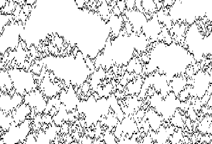
Figure 3: The mobility field of Fig. 2 is shown without the molecule trajectories. We are left with compact domains of immobility (white surfaces, the “bubbles” mentioned in the title of the paper), delimited by excitation lines shown in black.

In Fig. 3, one observes diffusion, creation and coagulation of mobility defects p3 . Therefore, trajectories look like a mixture of compact domains of immobility (white domains in Fig. 3), separated by excitation lines (black lines). These white domains are the bubbles mentioned in the title of the paper. We now list a number of canonical features that directly and generically follow from the bubble structure of the trajectories of the mobility field.

III.1 (Super-)Activated dynamical slowing down

From the trajectories of the molecules shown in Fig. 2, it it evident that the mean temporal extension of the bubbles represents a good measure of the structural relaxation time of the system, usually noted $\tau_{\alpha}(T)$, where $T$ is the temperature. In terms of the mobility field, a natural correlator is the local persistence, $P(x,t)$, from which $\tau_{\alpha}$ can be readily evaluated p4 . It is found that $\tau_{\alpha}(T)$ rapidly increases when $T$ is decreased. In the simple case of the $d=1$ FA model, Arrhenius behaviour is found, while super-Arrhenius behaviour can be found in more constrained models sollich . The dynamical slowing down results from the fact that mobility is locally needed to facilitate the dynamics, but the mean mobility decreases at $T$ decreases. Note the essentially non-mean-field character of this mechanism for relaxation that relies on local fluctuations of the mobility which will be hardly captured by mean-field treatments szamel .

III.2 Broad distributions of relaxation times

From Fig. 3, it is evident that the time extension of the bubbles is very broadly distributed, with small bubbles coexisting in space with very large ones. Calculations show that the time decay of $\langle P(x,t)\rangle$ is described, at low temperatures, by a stretched exponential form p3 ; p4 ,

$$\langle P(x,t)\rangle=\exp\left[-\left(\frac{t}{\tau_{\alpha}(T)}\right)^{\beta}\right],$$ (4)

where the stretching exponent is constant, $\beta=1/2$, for the $d=1$ FA model, but can be temperature dependent in more constrained dynamics. Therefore, the commonly used stretched exponential form (4) is a natural consequence of the spatial heterogeneity observed in Fig. 3. Moreover, detailed studies of the distributions of relaxation times reveal many additional features at intermediate times or temperatures, that compare well to simulations and experiments p25 ; p6 .

III.3 Thermodynamics

In this approach, thermodynamics is trivially given by that of a non-interacting gas of point defects. For the FA Hamiltonian, one gets the mean mobility

$$c(T)\equiv\langle\varphi\rangle=\frac{1}{1+\exp(1/T)},$$ (5)

and the free energy, $f(T)=-T\ln{\left(1+e^{-1/T}\right)}$.

A traditional quantity characterizing the loss of ergodicity taking place experimentally at the glass temperature, $T_{g}$, is the jump in specific heat $\Delta C_{p}$. The configurational contribution to this jump can be readily estimated within this approach from the free energy,

$$\Delta C_{p}(T_{g})\approx\left(\frac{J}{T_{g}}\right)^{2}{\cal N}c(T_{g}),$$ (6)

where $J$ sets the energy scale of the non-interacting Hamiltonian, and ${\cal N}\propto V_{x}$ is the number of molecules that contribute to enthalpy fluctuations per mobile cell, cf Eq. (2). This shows that the concentration of mobile regions at $c(T)$ plays again the key role, since the jump in specific heat is given in this approach by the number of defects that freeze at $T_{g}$. Formula (6) was successfully used in Ref. p1 to analyze experimental data for the jump in specific heat. Other thermodynamic aspects of supercooled liquids remain to be studied within this approach.

III.4 Topography of the potential energy surface

The potential energy surface of glass-forming liquids is an object of study which attracted a lot of attention in recent years review2 . It was shown in Ref. p5 that the kinetically constrained approach reviewed here is instead characterized by a trivial potential energy surface. However, this highly dimensional space is associated to a non-trivial metric so that displacements are performed, at low temperatures, along its geodesics which may be highly non-trivial. In physical terms, this implies once more that dynamical trajectories capture the specificities of the physics, which are ignored if only the statics is considered.

A detailed analysis of local minima and saddles of the potential energy surface of kinetically constrained models was performed in Refs. p4 ; p6 , based on the analysis of trajectories similar to Fig. 3. The results are in nice agreement with known numerical studies of molecular liquids. This analysis provides therefore a consistent physical interpretation in the “real space” of the topography found numerically in liquids. Interestingly, this interpretation contradicts on several key aspects the current popular views of the mechanisms of relaxation of supercooled liquids, see Ref. p6 for a more exhaustive description.

In particular, it was found that reports of several changes of mechanisms supposedly arising at the so-called “mode-coupling singularity temperature”, $T_{c}$ mct , in fact result from a biased interpretation of numerical data, as already discussed by several groups review3 ; o1 ; o2 ; o3 ; o4 . These results cast some doubts on the existence of a physically meaningful crossover temperature $T_{c}$ defined from a quantitative use of the mode-coupling theory of the glass transition, and indicate that the topographic “confirmations” of a change of mechanism of diffusion near $T_{c}$ might be spurious.

Similarly, it is found that the configurational entropy is always a positive quantity for all $T>0$ ritort . Therefore there is no Kauzmann temperature, $T_{K}>0$, where the configurational entropy vanishes. However, the shape of $S_{c}(T)$ explains in simple terms why numerical or experimental extrapolations might lead to an apparent finite Kauzmann temperature. In this view, the “Kauzmann paradox” arises simply because an invalid extrapolation is performed.

III.5 Spatially heterogeneous dynamics

Dynamics in Fig. 3 is evidently spatially heterogeneous. The fact that kinetically constrained models are heterogeneous was noted long ago by Harrowell and coworkers h1 ; h2 ; h3 ; h4 .

First, it is obvious that different parts of the same system possess, at a given time, very different dynamics. Secondly, it is clear that two sites belonging to the same bubble have similar dynamics, while two sites belonging to far away bubbles don’t. This implies the existence of spatial dynamical correlations, and therefore of a dynamic correlation length, $\ell(T)$, which is given by the mean spatial extension of the bubbles. These correlations can be quantified through the following dynamic structure factor p3 ; p6 ,

$$S(q,t)=\int d^{d}x\,e^{iq\cdot x}\left[\langle P(0,t)P(x,t)\rangle-\langle P(x,t)\rangle^{2}\right],$$ (7)

which quantifies spatial correlations of the local dynamics. This structure factor is built from two-time, two-point objects, and appears to be the minimal correlator to study bubbles, which are indeed spatio-temporal domains.

In the $d=1$ FA model, it is found that $\ell(T)\sim c^{-1}(T)$, while more complex scaling forms can be obtained in other models p25 ; p8 ; p9 . Again, features such as “stringy” clusters string , increasing “four-point” susceptibilities silvio , non-Gaussian particle displacements weeks ; blaad , or results from single molecule experiments vandenbout can be easily accounted for by a detailed analysis of Fig. 3, see Refs. p25 ; p3 ; p8 ; p9 ; p7 .

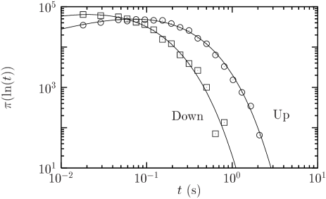
Figure 4: The points are distributions of flipping times for the molecular polarizations in supercooled polyvinylacetate recorded at the nanometer scale with an AFM tip by Vidal-Russel and Israeloff isr . The full lines are theoretical fits using Eq. (8) derived from the theoretical approach discussed in this paper which perform much better than the original phenomenological fit used in isr .

As a single concrete example, we present in Fig. 4 experimental data obtained by Vidal-Russel and Israeloff isr . In this experiment, time series of molecular polarizations are recorded with an AFM tip. This means that the dynamics of a very small volume is accessed, typically $(20\,{\rm nm})^{3}$ isr . Translated in our language, this experimental setup probes fluctuations at the scale of a few bubbles. The full lines in Fig. 4 are a fit using the distribution of relaxation times found in kinetically constrained spin models,

$$\pi(t)=\frac{1}{\tau_{\alpha}(T)\cal N}\left(\frac{t}{\tau_{\alpha}(T)}\right)^{\beta-1}\exp\left[-\left(\frac{t}{\tau_{\alpha}(T)}\right)^{\beta}\right],$$ (8)

where $\cal N$ normalizes the distribution, $\int dt\,\pi(t)=1$. It is interesting to note that the power law prefactor was omitted in the original experimental paper, but is necessary for a successfull fit of the whole experimental distributions p4 .

III.6 Decoupling and diffusion

We end our short tour of the phenomenology of supercooled liquids with the phenomenon of decoupling, which attracted a lot of attention in the last decade. It was indeed discovered at the beginning of the 90’s that the temperature dependences of various dynamic measures of the relaxation time of a given liquid do not necessarily coincide. In particular, viscosity, $\eta\sim\tau_{\alpha}$, and diffusion constant, $D$, have temperature dependences which result in a breakdown of the phenomenological Stokes-Einstein relation between these two quantities dec1 ; dec2 ; dec3 .

Once again, Fig. 2 provides a simple explanation of this result, as was in explained in full detail in Ref. p2 . We observe indeed that once trapped, it takes a long time to particles to start to move, which happens when they are hit by a diffusing defect. However, once in movement, particles can make several moves very rapidly because they might be “advected” by the diffusing defects. Schematically, this means that a major bottleneck for diffusion is the first move, but once in movement diffusion takes place on a much shorter time scale. Since viscosity is roughly associated to the first move, while diffusion averages over many, decoupling naturally follows.

Quantitatively, it is found for the $d=1$ FA model that $\tau_{\alpha}(T)\sim c^{-3}(T)$, while $D(T)\sim c^{2}(T)$, so that the product $D\tau_{\alpha}$ is not constant but rapidly increases when $T$ decreases, as found in experiments. Quantitative predictions for $d=3$ systems of various fragilities can also be found in Ref. p2 .

This decoupling phenomenon is again a direct consequence of the structure of trajectories shown in Fig. 3. Note that decoupling might arise even in a case where distributions of time scales do not broaden as $T$ decreases. In the $d=1$ FA model, for instance, $\pi(t,T)=\Pi(t/\tau_{\alpha}(T))$. This directly contradicts the naive argument very often put forward that since $D$ and $\eta$ correspond to different averages, respectively to $\langle t^{-1}\rangle$ and $\langle t\rangle$, over broader and broader distributions, they have different $T$-dependences dec4 . This is actually a crucial point since it may help to discriminate various approaches. Experimentally, decoupling is indeed found in a system for which distributions do not broaden dec3 .

Finally, note that naive dimensional analysis using the Stokes-Einstein relation allows one to define a “Stokes” length scale, $a$, via dec2 ; dec5

$$a\sim\frac{T}{D\eta},$$ (9)

which decreases when $T$ decreases. This is apparently puzzling since spatial correlations increase when $T$ decreases. In fact, it was recently showed by a statistical treatment of the trajectories shown in Fig. 1 that a different dimensional analysis in fact holds p7 . Since $\eta\sim\tau_{\alpha}$, it is possible to define a “diffusive” length scale, $\ell^{\star}$, as p7

$$\ell^{\star}\sim\sqrt{D\eta},$$ (10)

which increases when $T$ decreases. This length scale has a simple physical meaning p7 : it is the length scale beyond which Fickian diffusion holds. This new length scale was recently observed in a numerical experiment of an atomistic supercooled liquid ellstar , and experimentally in supercooled liquid TNB mark .

IV The zero-temperature dynamic critical point

The previous section was mainly qualitative since we discussed physics from a “pictorial” point of view, in order to convince readers that the bubble picture shown in Fig. 3 contains interesting physical informations when thoroughly analyzed.

In order to get a quantitative theory on top of a pleasant physical scenario, one has to arrive at quantitative predictions for three-dimensional systems. In this approach, this means being able to solve $d=3$ coarse-grained kinetically constrained models. Moreover, exact solutions of simple models have always played an inspiring role in statistical mechanics in general, the literature of glassy systems being no exception.

Recently, the $d=3$ version of the FA model described above was studied using a dynamic field-theoretic approach p8 ; p9 . This approach is justified since we already mentioned several times that the physics in these models is governed by increasing time and length scales, so that a continuous field theory can a priori prove useful. Moreover, the bubbles discussed above are the result of a reaction-diffusion type of process in terms of the point defects of mobility. Reaction-diffusion problems are usually described field-theoretically, the large scale properties being studied using the renormalization group review . This is the path followed in Refs. p8 ; p9 . In $d=1$, however, the problem can instead be mapped to interacting quantum spins, and again be studied with real space renormalization procedures p30 .

In $d=3$, the problem is solved in two steps. First, one has to derive a continuous field theory describing the physics. This is done using standard techniques, starting from a discrete master equation for the mobility, and ending with a continuous action. For a non-conserved mobility field, and a dynamic constraint as in Eq. (3), one gets the following action,

$$\mathcal{S}[\bar{\varphi},\varphi,t_{0}]=\int d^{d}x\,\int_{0}^{t_{0}}dt{\big{\lgroup}}\bar{\varphi}\left(\partial_{t}-D_{0}\nabla^{2}-\kappa_{0}^{(m)}\right)\varphi$$ (11)

$$+\bar{\varphi}\varphi(\lambda_{0}^{(1)}+\nu_{0}^{(1)}\nabla^{2})\varphi+\bar{\varphi}\varphi(\lambda_{0}^{(2)}+\nu_{0}^{(2)}\nabla^{2})\bar{\varphi}\varphi$$

$$-\bar{\varphi}\varphi(\kappa_{0}^{(v)}+\sigma_{0}\nabla^{2})\bar{\varphi}{\big{\rgroup}},$$

In this expression, $\varphi(x,t)$ can be thought of as a continous mobility field, while $\bar{\varphi}(x,t)$ stands for its conjugated response field. Several coupling constants have also been introduced, see p8 . Since the hypothesis to derive (11) are the same as in the FA model, we expect that both models belong to the same universality class.

The large scale properties of the action are then analyzed in detail. The action (11) has the form of a single species branching and coalescing diffusion-limited reaction with additional momentum dependent terms review . By integrating out the response field, a Langevin equation for the evolution of $\varphi$ is obtained. This equation has a critical point at $c=0$, i.e. $T=0$, describing the crossover from an exponential decay of mobility at finite $c$, i.e. $T>0$, to an algebraic decay at $c=0$. In the absence of noise, corresponding to neglecting terms quadratic in $\bar{\varphi}$, (11) admits the Gaussian exponents $(\nu_{\perp}^{G},\nu_{\parallel}^{G},\beta^{G})=(\frac{1}{2},1,1)$. Here $\nu_{\perp}$ and $\nu_{\parallel}$ control the growth of spatial $(\xi_{\perp})$ and temporal $(\xi_{\parallel})$ length scales near criticality, $\xi_{\perp}\sim c^{-\nu_{\perp}}$ and $\xi_{\parallel}\sim c^{-\nu_{\parallel}}$, while $\beta$ governs the long-time scaling of the energy density, $n\sim c^{\beta}$.

These Gaussian power laws are modified by fluctuations which are treated using the RG. It is found that the critical point remains at $c=0$. There is thus no finite temperature phase transition. Dimensional analysis shows that the upper critical dimension of the model is $d_{c}=4$. For $d\leq 4$ fluctuations are accounted by studying the behaviour of the effective couplings. For $1<d\leq 4$, all interaction terms in (11) except for $\lambda^{(1)}$ and $\kappa^{(v)}$ are irrelevant. It follows that our system is described for intermediate length and time scales by the directed percolation (DP) critical point and its associated power laws review . To order $\epsilon=d_{c}-d$ they are $(\nu_{\perp},\nu_{\parallel},\beta)=(\frac{1}{2}+\frac{\epsilon}{16},1+\frac{\epsilon}{12},1-\frac{\epsilon}{6})$.

This analysis implies that the slowdown is a dynamical critical slowing down as the critical point is approached from above. Correlation time and length scales grow as inverse powers of $c$. Thermal activation results from $c\sim e^{-1/T}$. Dynamical scaling is predicted to occur when the dynamic correlation length becomes appreciably larger than the lattice spacing. This happens therefore for temperatures lower than $T_{o}$, the onset temperature for dynamic heterogeneity p6 ; Brumer-Reichman .

These analytical results apply to systems with isotropic dynamic facilitation. They are therefore expected to apply to strong liquids, and to those which exhibit a crossover from fragile to strong behaviour p1 . While DP behaviour is not expected for the case of anisotropic constraints or conserved order parameters p25 ; p9 , a zero-temperature critical point is likely to be a generic feature of both strong and fragile glass formers p8 ; p9 ; Aldous-Diaconis-Toninelli-et-al , so that scaling properties of liquids in their fragile regime can also be described by a field theory p9 . Criticality also implies that techniques used to study continuous phase transitions, such as finite size scaling, can be employed to study the glass transition fss .

This field theorical approach suggests the following physical picture. The viscosity of a supercooled liquid increases rapidly as $T$ is lowered, because the dynamics becomes increasingly spatially correlated. A glass is obtained when the liquid’s relaxation time exceeds the experimental time scale. The scaling properties of time and length scales and therefore the physical properties of supercooled liquids are governed by a zero temperature dynamic critical point. It was therefore proposed that this critical point is responsible for the experimental existence of the glass state p8 .

V Conclusion

In this paper, I have very briefly summarized a recent series of papers dedicated to the derivation and analysis of a coarse-grained approach to the physics of supercooled liquids. The main idea is to map the liquid’s degrees of freedom onto a mobility field. After coarse-graining, simple empirical rules are used to specify the dynamics of the mobility field, resulting in well-defined models, that are simple enough that a number of analytical results can be derived. I have shown that a wide number of physical quantities can then be deduced from the statistical properties of the mobility field, leading to a consistent theoretical description of all aspects of glass transition phenomena.

The generic scenario is that the glass formation is driven by an underlying zero-temperature critical point where both timescales and lengthscales diverge, in the form of non-trivial dynamic correlations, the bubbles of Fig. 3. A key temperature scale in the problem is $T_{o}$, which marks the onset of slow dynamics. Physically, $T_{o}$ delimits the the critical region, $T\in[0,T_{o}]$, influenced by the $T=0$ critical point. Other popular crossover temperatures, such as $T_{c}$ and $T_{K}$, play no role in this approach. Interestingly, this approach contradicts on several important points alternative theories, so that numerics or experiments might clarify its status in a relatively near future.

References

- (1) M.D. Ediger, C.A. Angell and S.R. Nagel, J. Phys. Chem. 100, 13200 (1996).
- (2) P.G. Debenedetti and F.H. Stillinger, Nature 410, 259 (2001).
- (3) G. Tarjus and D. Kivelson, in Jamming and Rheology, Eds: A.J. Liu and S.R. Nagel (Taylor and Francis, New York, 2001).
- (4) J.P. Garrahan and D. Chandler, Proc. Natl. Acad. Sci. USA 100, 9710 (2003).
- (5) Y.J. Jung, J.P. Garrahan, and D. Chandler, Phys. Rev. E 69, 061205 (2004).
- (6) L. Berthier and J.P. Garrahan, cond-mat/0410076.
- (7) J.P. Garrahan and D. Chandler, Phys. Rev. Lett. 89, 035704 (2002).
- (8) L. Berthier and J.P. Garrahan, J. Chem. Phys. 119, 4367 (2003).
- (9) L. Berthier and J.P. Garrahan, Phys. Rev. E 68, 041201 (2003).
- (10) S. Whitelam and J.P. Garrahan, J. Phys. Chem. B 108, 6611 (2004).
- (11) S. Whitelam, L. Berthier, and J.P. Garrahan, Phys. Rev. Lett. 92, 185705 (2004).
- (12) S. Whitelam, L. Berthier, and J.P. Garrahan, cond-mat/0408694.
- (13) L. Berthier, D. Chandler, and J.P. Garrahan, cond-mat/0409428.
- (14) S. Whitelam and J.P. Garrahan, Phys. Rev. E (in press); cond-mat/0405647.
- (15) L. Berthier, Phys. Rev. Lett. 91, 055701 (2003).
- (16) J.-L. Barrat and J.-P. Hansen, Basic concepts for simple and complex fluids (CUP, Cambridge, 2003).
- (17) F.H. Stillinger and T.A. Weber, Phys. Rev. A 25, 978 (1982); Phys. Rev. A 28, 2408 (1983); Science 225, 983 (1984).
- (18) T.B. Schrøder, S. Sastry, J.C. Dyre, and S.C. Glotzer, J. Chem. Phys. 112, 9834 (2000).
- (19) C.Y. Liao and S.-H. Chen, Phys. Rev. E 64, 031202 (2001).
- (20) J. Jäckle and S. Eisinger, Z. Phys. B 84, 115 (1991).
- (21) G.H. Fredrickson and H.C. Andersen, Phys. Rev. Lett. 53, 1244 (1984).
- (22) R.G. Palmer, D. L. Stein, E. Abrahams, and P.W. Anderson, Phys. Rev. Lett. 53, 958 (1984).
- (23) J. Jäckle, J. Phys. C: Condens. Matter 14, 1423 (2002).
- (24) F. Ritort and P. Sollich, Adv. in Phys. 52, 219 (2003).
- (25) G. Szamel, J. Chem. Phys. 121, 3355 (2004).
- (26) W. Götze and L. Sjögren, Rep. Prog. Phys. 55, 55 (1992).
- (27) J.P.K. Doye and D.J. Wales, J. Chem. Phys. 116, 3777 (2002).
- (28) B. Doliwa and A. Heuer, Phys. Rev. E 67, 031506 (2003).
- (29) R.A. Denny, D.R. Reichman, and J.-P. Bouchaud, Phys. Rev. Lett. 90, 025503 (2003).
- (30) X.C. Zeng, D. Kivelson, and G. Tarjus, Phys. Rev. E 50, 1711 (1994).
- (31) A. Crisanti, F. Ritort, A. Rocco, M. Sellitto, J. Chem. Phys. 113, 10615 (2000).
- (32) S. Butler and P. Harrowell, J. Chem. Phys. 95, 4454 (1991).
- (33) S. Butler and P. Harrowell, J. Chem. Phys. 95, 4466 (1991).
- (34) P. Harrowell, Phys. Rev. E 48, 4359 (1993).
- (35) M. Foley and P. Harrowell, J. Chem. Phys. 98, 5069 (1993).
- (36) C. Donati, J.F. Douglas, W. Kob, S.J. Plimpton, P.H. Poole, and S.C. Glotzer, Phys. Rev. Lett. 80, 2338 (1998).
- (37) S. Franz and G. Parisi, J. Phys. C 12, 6335 (2000); S.C. Glotzer, J. Non-Cryst. Solids 274, 342 (2000).
- (38) W.K. Kegel and A. van Blaaderen, Science 287, 290 (2000);
- (39) E.R. Weeks, J.C. Crocker, A.C. Levitt, A. Schofield, and D.A. Weitz, Science 287, 627 (2000).
- (40) L.A. Deschenes and D.A. Vanden Bout, Science 292, 255 (2001).
- (41) E. Vidal Russell and N.E. Israeloff, Nature 408, 695 (2000).
- (42) F. Fujara, B. Geil, H. Sillescu, and G. Fleischer, Z. Phys. B 88, 195 (1992).
- (43) J.-L. Barrat, J.-N. Roux, and J.-P. Hansen, Chem. Phys. 149, 197 (1990).
- (44) S.F. Swallen, P.A. Bonvallet, R.J. McMahon, and M.D. Ediger, Phys. Rev. Lett. 90, 015901 (2003).
- (45) G. Tarjus and D. Kivelson, J. Chem. Phys. 103, 3071 (1995).
- (46) P. Bordat, F. Affouard, M. Descamps, and F. Müller-Plathe, J. Phys.: Condens. Matter 15, 5397 (2003).
- (47) L. Berthier, Phys. Rev. E 69, 020201(R) (2004).
- (48) M. Ediger et al., unpublished.
- (49) H. Hinrichsen, Adv. Phys. 49, 815 (2000).
- (50) Y. Brumer and D.R. Reichman, Phys. Rev. E 69, 041202 (2004).
- (51) This has also been shown rigorously to be the case for the East model east in D. Aldous and P. Diaconis, J. Stat. Phys. 107, 945 (2002) and the Kob-Andersen lattice model KA in C. Toninelli, G. Biroli and D.S. Fisher, Phys. Rev. Lett. 92, 185504 (2004).
- (52) W. Kob and H.C. Andersen, Phys. Rev. E 48, 4364 (1993).