Quasi-2D Confinement of a BEC in a Combined Optical and Magnetic Potential

Abstract

We have added an optical potential to a conventional Time-averaged Orbiting Potential (TOP) trap to create a highly anisotropic hybrid trap for ultracold atoms. Axial confinement is provided by the optical potential; the maximum frequency currently obtainable in this direction is 2.2 kHz for rubidium. The radial confinement is independently controlled by the magnetic trap and can be a factor of 700 times smaller than in the axial direction. This large anisotropy is more than sufficient to confine condensates with $\sim 10^{5}$ atoms in a Quasi-2D (Q2D) regime, and we have verified this by measuring a change in the free expansion of the condensate; our results agree with a variational model.

I Introduction

Two-dimensional systems are of great interest in condensed matter physics in general, and they have some special properties Binney et al. (1992),Cardy (1996). A two-dimensional Bose gas confined in a uniform potential does not undergo Bose-Einstein condensation (BEC); instead there is a Berezinskii-Kosterlitz-Thouless (KT) transition: a topological phase transition mediated by the spontaneous formation of vortex pairs which leads to a system that does not have long-range order but which is nevertheless superfluid. Many features of the KT transition have been observed in experiments with films of superfluid He⁴ on surfaces Bishop and Reppy (1978)Kosterlitz and Thouless (1973); (see Luhman and Hallock (2004) for some recent results). In experiments with a thin layer of spin-polarised atomic hydrogen gas on a liquid helium surface Safonov et al. (1998), evidence was found for the existence of a quasi-condensate: a system that only possesses local phase coherence, in contrast to a pure condensate that has a global phase.

The recent advent of laser cooling and subsequent Bose-condensation of the alkali metal atoms Anderson et al. (1995) has opened up a new avenue of investigation: while these bosonic gases are initially cooled to quantum degeneracy as three dimensional clouds, the addition of novel dipole force potentials can make these systems two dimensional to varying degrees. A condensate can be called quasi-two dimensional (Q2D) when the energy level spacing in one dimension exceeds the interaction energy between the atoms. In this case the particles obey 2D statistics but interact in the same way as in a three-dimensional system.

The first Q2D condensate was made with sodium atoms that were condensed in a magnetic trap and then loaded into an attractive optical dipole trap Gorlitz et al. (2001). The dipole trap was made by tightly focusing a laser beam along one direction with a cylindrical lens to achieve trap aspect ratios of 79. In this experiment the number of atoms, and hence the interaction energy, was reduced to enter the Q2D regime. A Q2D condensate of two thousand caesium atoms has also been made in a surface wave trap with an aspect ratio of 50 Rychtarik et al. (2004). In our experiment we use two sheets of blue-detuned light to increase the axial confinement of our magnetic trap, this approach allows anisotropies in excess of 700 to be achieved as the radial confinement is provided independently by the magnetic trap, which in turn allows more atoms to be loaded into the Q2D regime. The combination of our magnetic Time-averaged Orbiting Potential (TOP) trap and dipole potential creates a flexible system with the ability to rotate the condensate, so that vortex nucleation can also be studied.

Q2D condensates have many interesting properties that are not present in 3D: the effect of phase fluctuations has been examined theoretically in Petrov et al. (2000); the possibility of vortex production as a mechanism for the decay of a quadrupole mode is examined in Fedichev et al. (2003). Indeed while it has been shown that in a harmonically trapped non-interacting gas Bose-Einstein condensation can occur Bagnato and Kleppner (1991), there is still a question of when an interacting 2D system supports a KT rather than a BEC transition.

Our paper is structured as follows: in the second section we describe the design of our optical potential, in the third section we discuss its realisation and some initial calibration measurements, and in the final section we present our measurements of the condensate in free expansion which confirm it has been trapped in the Q2D regime.

II Dipole Trap Design

II.1 Optical Potential

In order to produce strong axial confinement, we trap the atoms in the nodal plane at the focus of a Hermite-Gaussian TEM₀₁-like mode. To produce this light field the output from a laser at wavelength $\lambda=532$ nm (Coherent Verdi) is passed through a phase-plate, which imprints the top half of the beam with a $\pi$ phase shift relative to the bottom half. The phase-plate was manufactured in house, and coated in such a way as to balance the reflective losses from the upper and lower surfaces. After focusing with a cylindrical lens with focal length $f=160~{}\text{mm}$ in the $z$ direction, the intensity pattern at the focus resembles a TEM₀₁ mode to a first approximation.

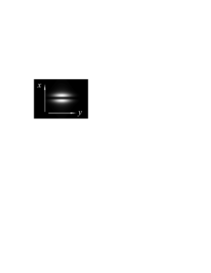
Figure 1: TEM₀₁-like intensity distribution at the focus of the final cylindrical lens. Axis convention is shown: $z$ is in the vertical direction, $y$ is horizontal across the beam and $x$ is along the direction of beam propagation, out of the page. The $y$ and $z$ directions are not to scale. The radial direction is to be interpreted as in the $xy$ plane.

We derive the exact expression for the intensity distribution below and also discuss any shortcomings together with the effects of various types of misalignment. The axis convention used in this paper is explained in Fig. 1 and the coordinate axes are denoted by capital letters for the input plane (at the position of the cylindrical lens) whereas they are denoted by small letters in the focal plane, where the atoms are trapped. The intensity distribution of the initial beam is given by

$$I_{\mathrm{init}}(Y,Z)=\frac{2P}{\sigma_{y}\sigma_{z}\pi}\exp{\left(-\frac{2Y^{2}}{\sigma_{y}^{2}}\right)}\exp{\left(-\frac{2Z^{2}}{\sigma_{z}^{2}}\right)},$$ (1)

where $\sigma_{y},\sigma_{z}$ are the beam waists in $Y$ and $Z$ direction, respectively, and $P$ is the power in the laser beam. The amplitude function $\tilde{\phi}(y,z)$ in the focal plane is given by

$$\tilde{\phi}(y,z)=\frac{1}{\sqrt{\lambda f}}\int_{-\infty}^{\infty}\exp\left(\mathrm{i}\tilde{k}Z\right)\phi(y,Z)dZ,$$ (2)

where $\phi(y,Z)=\phi(Y,Z)=\sqrt{I_{init}(Y,Z)}~{}\gamma(Z-Z_{0})$ is the amplitude function in the input plane. The function $\gamma(Z-Z_{0})=1$ for $Z<Z_{0}$ and $\gamma(Z-Z_{0})=-1$ for $Z>Z_{0}$. It represents the action of the phase-plate which, as we shall assume in the following, is aligned with the center of the Gaussian beam for $Z=Z_{0}$. The cylindrical lens performs a 1-d Fourier transform and $\tilde{k}=kz/f$, $k=2\pi/\lambda$. After some calculations we obtain for the intensity in the focal plane

$$I_{\mathrm{foc}}(y,z)=\left|\tilde{\phi}(y,z)\right|^{2}$$ (3)

$$=\frac{2P}{\lambda f}\frac{\sigma_{y}}{\sigma_{z}}\text{erfi}\left(\frac{k\sigma_{z}z}{2f}\right)^{2}\exp\left(-\frac{k^{2}\sigma_{z}^{2}z^{2}}{2f^{2}}\right)\exp\left(-\frac{2y^{2}}{\sigma_{y}^{2}}\right),$$

where the imaginary error-function $\text{erfi}(z)$ is defined in terms of the conventional error function $\text{erf}(z)$ evaluated for a purely imaginary argument: $\text{erfi}(z)=-\mathrm{i}~{}\text{erf}(\mathrm{i}z)$. To first order $\text{erfi}(z)\approx(2/\sqrt{\pi})z+O(z^{3})$. Inserting this approximation to erfi into the above equation and expanding it up to second order in $z$ we obtain

$$I_{\mathrm{foc}}(z)=\frac{8\pi P\sigma_{z}^{3}}{\lambda^{3}f^{3}\sigma_{y}}z^{2}+O(z^{4}).$$ (4)

Provided that $\Delta\gg\Delta_{FS}$ Grimm et al. (2001), where $\Delta$ is the detuning of the dipole trap from resonance with the atomic transition and $\Delta_{FS}$ is the fine structure splitting of the transition, the potential energy of an atom in the dipole trap is related to the intensity of the light field by

$$U_{\mathrm{dip}}(\textbf{r})=\frac{3\pi c^{2}}{2\omega_{0}^{3}}\frac{\Gamma}{\Delta}I(\textbf{r}),$$ (5)

where $c$ is the speed of light in vacuo, $\Gamma$ and $\omega_{0}$ are the linewidth and frequency of the atomic transition, and $I(\underline{r})$ is the intensity of the dipole trapping beam. In our experiment the atomic transition is the ${}^{2}S_{1/2}\rightarrow^{2}P_{1/2,3/2}$ in atomic Rb⁸⁷ which has a wavelength of 780 nm. From Eqs.(4,5) we obtain for the axial trap frequency $\Omega$ for atoms of mass $m$,

$$\Omega^{2}=\frac{24\pi^{2}P\sigma_{z}^{3}c^{2}\Gamma}{\lambda^{3}f^{3}\sigma_{y}\omega_{0}^{3}m\Delta}.$$ (6)

Going back to Eq.(3) we shall define the beam waists in the focal plane as $w_{y}=\sigma_{y}$ and $w_{z}=2f/(k\sigma_{z})$. The latter relation is exactly that between the input and the output waists of a Gaussian beam. A Gaussian beam of any order transforms into different sized Gaussian beam of the same order through the action of a lens. In our case the phase jump introduced by the phase-plate causes a zeroth order Gaussian to transform into something closely resembling a first order Gaussian beam (TEM₀₁) rather than a zeroth order. Using the expressions for the beam waists in the focal plane the intensity profile (3) can be written as

$$I_{\mathrm{foc}}(y,z)=$$

$$\frac{2P}{\pi w_{y}w_{z}}\text{erfi}\left(\frac{z}{w_{z}}\right)^{2}\exp\left(-\frac{2z^{2}}{w_{z}^{2}}\right)\exp\left(-\frac{2y^{2}}{w_{y}^{2}}\right).$$ (7)

The axial trap frequency $\Omega$ can then be expressed in terms of these waists as

$$\Omega^{2}=\frac{24c^{2}\Gamma P}{\pi m\omega_{0}^{3}w_{z}^{3}w_{y}\Delta}.$$ (8)

In order to determine the trap frequency $\Omega$ for our experimental parameters we can measure the TEM₀₀ profile in the input plane and then use Eq.(6) to calculate the resulting trap frequencies of the optical potential in the focal plane. Alternatively, we can measure the distance $d_{z}$ between the two intensity peaks in the focal plane and use the relation $d_{z}=1.8483~{}w_{z}$ to determine $\Omega$ from Eq.(8). The beam intensity profile, given by Eq.(3) differs somewhat from that of a perfect TEM₀₁ which is given by

$$I_{\mathrm{TEM_{01}}}(y,z)=\frac{8P}{\pi w_{z}^{3}w_{y}}z^{2}\exp{\left(-\frac{2z^{2}}{w_{z}^{2}}\right)}\exp{\left(-\frac{2y^{2}}{w_{y}^{2}}\right)}.$$ (9)

Substituting $\text{erfi}(z)\approx 2/(\sqrt{\pi})z$ into Eq.(7) we obtain Eq.(9) with the initial multiplying constant smaller by a factor of $\pi$. This approximation is only valid for small $z$ but it indicates that in the central region, where we want to confine the atoms, the intensity of the focused beam is reduced by a factor of $\pi$ with respect to that of a pure TEM₀₁ beam of the same power $P$. The reason is that much power is lost in the very broad wings of the focused beam which are much larger than those of a pure TEM₀₁. This can be seen in Fig.2a, where the solid line shows the actual potential given by Eq.(7) and the dotted line shows the potential of a TEM₀₁ given by Eq.(9) for comparison.

The initial amplitude distribution has a sudden jump in the middle where the amplitude goes from negative to positive. The focusing lens performs a Fourier transform and in order to resolve the sudden change in amplitude many higher spatial frequencies, represented by the wings of the intensity profile in the focus, are needed.

Combining the magnetic with the optical potential we find that the central position of the combined potential, in the axial direction, is given by

$$z_{c}(t)=\frac{z_{l}}{1+\frac{\omega_{m}^{2}}{\omega_{l}^{2}(t)}},$$ (10)

where $z_{c}$ is the position of the combined potential relative to the center of the magnetic trap, $z_{l}$ is the position of the center of the optical potential, and $\omega_{l}$ and $\omega_{m}$ are the angular frequencies of the optical and magnetic potentials respectively.

II.2 Beam Shaping and Misalignment Errors

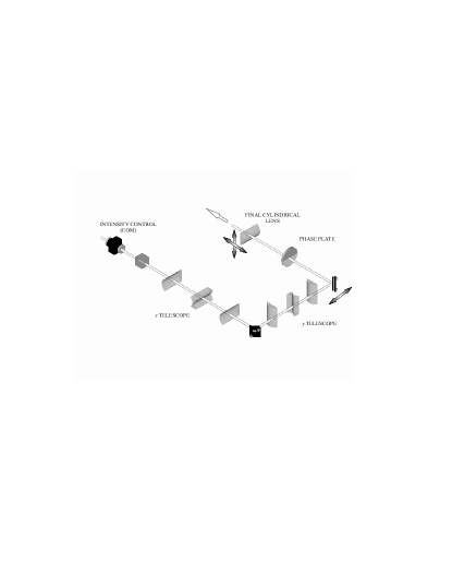
Figure 3: Schematic drawing of optical layout showing the cylindrical telescopes, the $\pi$ phase-plate and the final cylindrical lens. Shaded arrows indicate the location of sub-micron actuators for positional control over the focus.

A schematic diagram of the experimental setup is shown in Fig. 3. To achieve a high axial confinement frequency, a tight focus is required in the $z$ direction, as such the beam is expanded in this direction prior to focusing. A suitable choice of beam width is also required in the $y$ direction to determine the area in the $xy$ plane throughout which Q2D confinement can be realized. The $y$ and $z$ beam widths are not the same, and so some method of asymmetric beam expansion is required: for this experiment two orthogonal, cylindrical telescopes are used. To achieve a beam focus of 7.2 $\mu$m with a final lens of focal length f=160 mm, the beam waist in the $z$ direction before focusing must be 3.8 mm. The beam waist in the $y$ direction is chosen to be 410 $\mu$m. From Eq. (6) the resulting axial trap frequency is $\approx 2.7\text{kHz}$.

The potential height and frequencies are decreased by misaligning the phase-plate with respect to the incoming Gaussian beam. Two types of misalignment can occur. The first one is displacement of the phase step on the phase-plate from the center of the Gaussian beam. In this case $Z_{0}$, defined below Eq.(2), is not equal to zero. As a result the intensity dip in the central region is fills up for large values of the displacement parameter $\xi=Z_{0}/\sigma_{z}$. Fig. 2b shows a series of potential plots for various values of $\xi$. The central dip has completely disappeared for $\xi=1.5$. The resulting change in trap frequencies is shown in Fig. 4 (solid line) which plots $\Omega$ normalised by its value when $\xi=0$. The dotted line plots the potential height normalised by its value for $\xi=0$: $\Delta_{pot}=(I_{max}(\xi)-I_{min}(\xi))/(I_{max}(0)-I_{min}(0))$.

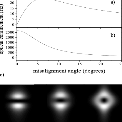
Figure 5: The effect of angular misalignment between the input beam and the final lens, calculated for $w_{z}$=7.2 $\mu$m and $P=4.5$ W. (a) Plot shows the confinement in the $y$ direction as a function of angular misalignment. (b) Plot shows decrease in axial trapping frequency as a function of misalignment. (c) Intensity distributions at the focus of the cylindrical lens for 2, 5 and 10 degrees of input beam misalignment (left to right; in all the plots the $y$ and $z$ axes are not the same scale).

The effect of rotational misalignments between the input beam, the phase-plate and the final cylindrical lens have been calculated numerically for our experimental parameters (see Fig. 5). The results show that the optical potential at the beam focus is relatively insensitive to the precise rotational alignment of the phase-plate; however, the angle that the elongated input beam makes with the cylindrical lens is much more critical, as misalignment decreases the axial confinement and introduces some radial confinement. In our experiment we aim to minimise the radial confinement and maximise the axial confinement provided by the optical potential.

III Experimental Realisation

III.1 Alignment

Sub-micron actuators give independent control over the focus of the optical potential in three dimensions. The $x$ and $z$ position of the focus can be controlled by moving the final cylindrical lens, and the $y$ position is changed by moving the position of a mirror which deflects the beam through 90 degrees (see Fig. 3). Intensity control is provided by an Electro-Optic Modulator (EOM).

The size and depth of the optical potential are too small to provide any noticeable change to the Magneto-Optical Trap (MOT) used in the first stage of our experiment, and so initial alignment was carried out by making the beam from a 397 nm semiconductor diode laser co-linear with the dipole trapping beam. Photons at this frequency are sufficiently energetic to ionize Rb atoms and deplete the MOT, providing a clear signature for alignment. Subsequent coarse alignment was carried out by lining up the MOT with the entry and exit reflections of the trapping beam on the glass cell. This allows the beam to be aligned to within  200 $\mu$m, in $x$ and $y$, of the magnetic trap center.

For the next stage of alignment the atoms were supported against gravity on top of the laser beam. The power in the trapping beam was then reduced, until the atoms were only just supported, and the beam moved in the $xy$ plane: as the beam focus is moved closer to the atoms, less power is required to stop the atoms from falling. This is an iterative process, which is accurate to $\sim 30~{}\mu m$ in $x$ and $y$.

The most critical direction for alignment in our experiment is the $z$ direction, which needs to be aligned to within a few microns to load atoms from the magnetic trapping potential into the dipole trap. Alignment in this direction exploits a delay that is required between the switch off of the magnetic and optical potentials. The dipole trap can be switched off by the EOM in a few microseconds, however the magnetic trap requires almost $500~{}\mu s$ before the current in the quadrupole coils decays. This can create a problem when looking at the expansion of condensates that are tightly confined by the optical potential: simulations show that when suddenly released, the expansion of the condensate can be slowed or even temporarily reversed by the residual magnetic fields. The solution is to introduce a delay of $500~{}\mu s$ after the magnetic field begins to decay, before switching off the optical potential. The equilibrium position of the atoms in the combined potential is not quite the same as the equilibrium position in the purely optical potential: the result is that the atoms move in the optical potential during the delay. The velocity they acquire during this period is sufficient after 15 ms of free expansion to allow the start position to be calculated, and is accurate to $\sim 1~{}\mu m$.

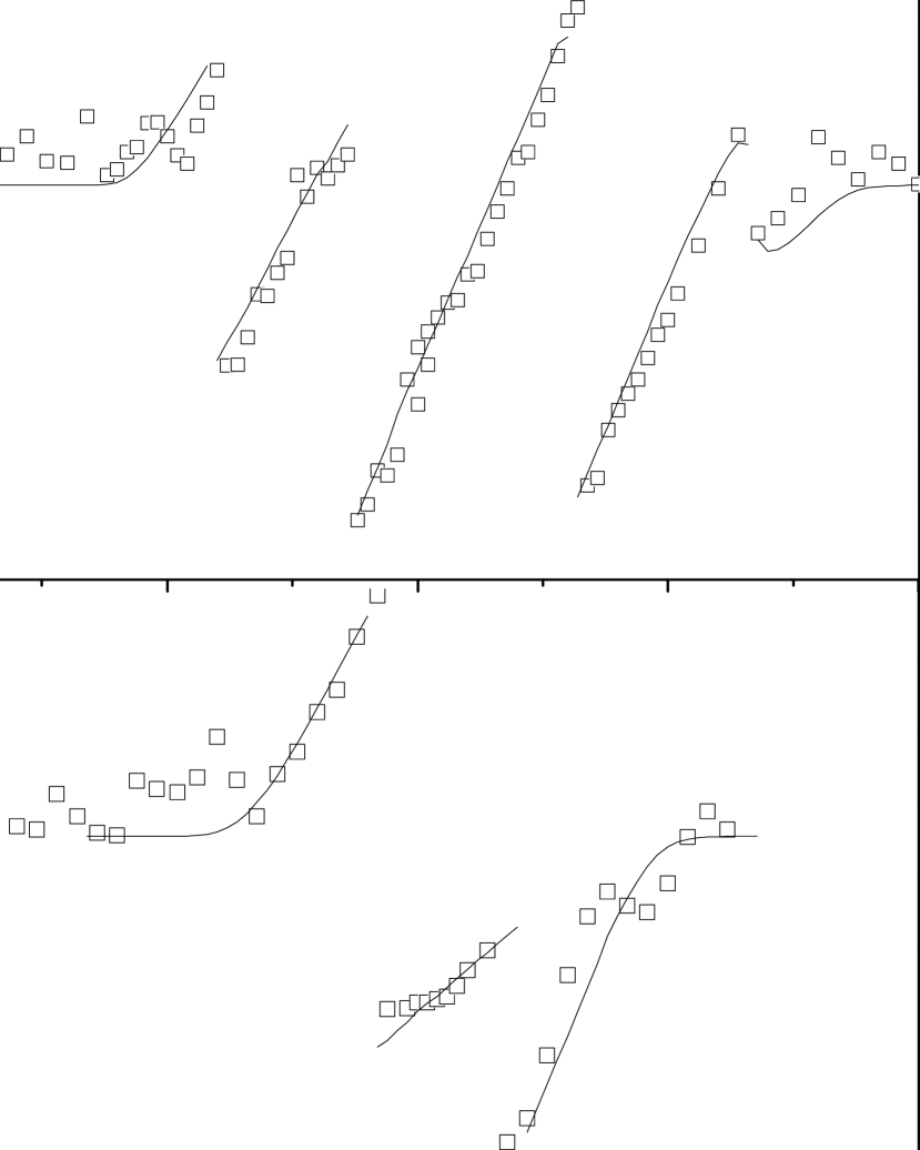
Figure 6: The position of the dipole trap beam is scanned in the $z$ direction, while the magnetic trap defining the initial position of the atoms, remains fixed. The dipole trap intensity is then ramped on and the position of the atoms observed after 15 ms of free expansion. (a)/(c) show a scan far from/closer to the focus of the trapping beam, ‘white squares’ are experimental points and the ‘solid line’ is the deflection expected for the potential in (b)/(d).

In Fig. 6 the position of the dipole trap beam is scanned in the $z$ direction, while the magnetic trap, which defines the initial position of the atoms, remains fixed. The dipole trap intensity is then ramped on and the position of the atoms observed after free expansion. Fig. 6(c) shows the pattern observed and expected for a TEM₀₁ potential, as shown in Fig. 6(d). The magnetic and dipole traps are only aligned in the central region of the plot in Fig. 6(c), this coincides with a sharp increase in the axial expansion of the condensate. The beam waist can be accurately measured from the width of the central region. This method can also be used to profile the beam at various points along its optical axis, and to partially reconstruct the intensity profile. Fig. 6(a) shows a scan further away from the beam focus, and Fig. 6(b) is an intensity pattern that produces the observed deflection.

III.2 Loading the Trap

Our experiment uses evaporative cooling in a TOP trap to create a Bose-condensate that contains $\sim 10^{5}$ atoms of the Rb⁸⁷ isotope in the $|F=1,m_{F}=-1\rangle$ state. The initial oscillation frequencies of atoms in the magnetic trap are 61 Hz radially and 172.5 Hz along the $z$ (axial) direction. After a condensate has been formed it is adiabatically loaded into the combined potential: the intensity of the dipole force laser beam is ramped from zero to its maximum value in 100-300 ms (depending on the strength of the optical potential). This ensures that no dipole modes, or internal modes of the condensate, are excited during the loading phase. This was confirmed by an exact numerical simulation. The combined central position changes most rapidly when the frequencies of the potentials are comparable (see Eq. 10), at the beginning of the ramp. For the highest frequency dipole traps this means that the ramp needs to be extended to give the condensate a smooth transition and avoid unnecessary heating.

III.3 Calibration

Dipole frequency measurements in the radial and axial directions are used to characterise the trap. For the highest frequency traps, the measurement is complicated because the TOP frequency (7 kHz) is comparable to the dipole frequency in the axial direction. Efforts to observe the dipole oscillation with the TOP field on were unsuccessful for this reason. It is therefore necessary to turn off the TOP field and move the quadrupole center above the optical potential, to avoid atom loss through Majorana spin flips. In this geometry it is necessary to suddenly change the quadrupole gradient to excite the dipole mode. We have measured an axial frequency of 2.2 kHz, as shown in Fig. 7, for a beam waist of 7.2 $\mu$m, determined from the deflection of atoms as previously explained. This agrees roughly with the expected value of 2.7 kHz for an ideal phase-plate profile, calculated using Eq. 6, when the rotational misalignment between the phase-plate and the final cylindrical lens is taken into account. A rotation by only $4\pm 1$ degrees effectively changes the axial frequency to $1.94\mp 0.27~{}\text{kHz}$. From the frequency measurement it is also possible to estimate the axial beam drift to be approximately 18 $\mu$m/hr. The radial trap frequencies have also been measured by exciting dipole modes, and by measuring the aspect ratio of the condensate (defined as $l_{y}/l_{x}$, where $l$ is the width of the condensate extracted from a Gaussian fit) in the $xy$ plane after free expansion. At high values of radial confinement from the magnetic trap, the dipole frequencies were as expected for a purely magnetic potential; however, as the magnetic confinement was reduced it was observed that the cloud elongated along the beam direction (see Fig. 8), and when the dipole mode was excited it oscillated only along the propagation direction of the trapping beam. In this direction the dipole oscillation frequency agrees with the expected value for a purely magnetic potential, but across the beam there is some extra confinement provided by the optical potential. The optical frequency along the $y$ direction was used as a fitting parameter for the data in Fig. 8: for a fixed optical frequency a curve was calculated for all the various magnetic frequencies and the resulting curve compared to the data points. This procedure was repeated to find the least squares minimum value for the optical potential. This was found to be equivalent to 26 Hz for an axial trapping frequency of 1990 Hz, and is caused by the rotational misalignment described above. Indeed subsequently we have measured the tilt of the input beam relative to the final cylindrical lens and found a value of $4\pm 1$ degrees, from Fig. 5 it can be seen that this theoretically gives between 19 and $23$ Hz of confinement.

We also measured the axial size of the condensate as a function of trapping beam power. The condensate expanded for 15 ms before it was imaged. The results are shown in Fig. 9 and are in good agreement with the hydrodynamic theory and the assumption that $\Omega\propto\sqrt{P}$, as would be expected for a harmonic dipole trap (see Eq. 6). These measurements were made at a radial frequency of 61 Hz and so the hydrodynamic expansion theory applies.

IV The Quasi-2D Regime

IV.1 Criterion for Q2D

The condition $\mu<\hbar\omega_{z}$, where $\mu$ is the chemical potential, can be used as a criterion for when a condensate is in the Q2D regime. In this case the ground state energy is smaller than the harmonic oscillator spacing and thus comparable to the harmonic oscillator ground state. When $\sim 10^{5}$ atoms have been loaded into our combined optical and magnetic potential the Q2D regime can be reached by either decreasing the number of atoms, or by adiabatically decreasing the radial confinement provided by the magnetic trap. In the following experiments we use the second approach, to provide more control. Along the $z$ direction the condensate shape becomes very similar to the Gaussian profile of an ideal gas. However, along the weakly confined $x$ and $y$ axes the condensate is characterised by the hydrodynamic parabolic shape. For the best description in terms of simple analytic functions it is therefore best to describe the condensate wavefunction as a hybrid of a parabolic and a Gaussian distrubution.

IV.2 Expansion of a Q2D gas

In our experiments we observed the condensate expansion in various regimes and the smooth transition from the hydrodynamic expansion characteristics Castin and Dum (1996) to those of a quasi-2D gas, which essentially expands like an ideal non-interacting gas in the direction of tight confinement. The results are shown in Fig. 10(a), where the open circles and filled circles are the data for traps with $\omega_{z}/2\pi=1990~{}\text{Hz}$ and 960 Hz respectively. The expansion time is constant at 15 ms and the radial trap frequency is varied to explore the transition to Q2D. These curves demonstrate clearly the ideal-gas like behaviour for the axial expansion in this limit. We compared our findings to those of theoretical predictions which were derived from variational models Perez-Garcia et al. (1996) and found good agreement to our data. The prediction of the hybrid variational model G.Hechenblaikner et al. , which is indistinguishable from that of the Gaussian variational model, is given by the solid line. The horizontal dashed lines indicate the expansion of the ideal gas, given by $R_{z}=t\sqrt{\hbar\omega_{z}/m}$, where $t$ is the expansion time, and the dotted lines the expansion of the hydrodynamic gas. The ‘ideal gas’ and hydrodynamic models yield straight lines on the logarithmic plot. In contrast, the curve for the hybrid model follows the hydrodynamic asymptote down to $\omega_{x}\approx 20~{}\text{Hz}$, corresponding to $\mu\approx\hbar\omega_{z}$, where it bends and follows the ‘ideal gas’ line towards zero radial frequency. The two noticeably do not coincide at $\omega_{x}\approx 0$ because of the residual optical anisotropy in the radial plane (as we discussed before in the text describing Fig. 8), which was taken into account in our variational model and is in good agreement with the experimental data. This transition from the hydrodynamic to the ‘ideal gas’ asymptote gives conclusive evidence of the gas entering the Q2D regime. The release energy of the condensate, calculated from the size after expansion, is also shown in Fig. 10(b): this tends towards the ideal gas limit of $\hbar\omega_{z}/4$ as $\omega_{x}$ is reduced. This is the vertical kinetic zero-point energy; all that is available if the confining potential is suddenly switched off.

V Conclusions and outlook

In these experiments we have studied the properties of quasi-2D condensates. To obtain the required geometry we increased the stiffness of the axial confinement by superimposing an optical potential on the existing magnetic trapping potential. The resulting trap was characterised in detail and we obtained confinement frequencies close to the theoretically expected values. We then studied the properties of Q2D condensates including their chemical potential and expansion characteristics. Our experimental observations agreed with theoretical predictions to confirm that we successfully entered the Q2D regime. This was the first experiment to explore the hydrodynamic-Q2D transition by gradually increasing the trap anisotropy instead of throwing atoms away as in previous work Gorlitz et al. (2001). In future experiments we hope to study the properties of vortices and vortex arrays in the Q2D regime and investigate the possibilities of observing a Berezinskii-Kosterlitz-Thouless transition and studying its properties.

Figure 2: (a) The intensity distribution in the focal plane for the actual experimental setup (solid line) and for the ideal TEM₀₁ profile (dotted line) of the same total power. (b) The actual potential is plotted for various values of the displacement parameter: $\xi=0.3$ (solid line), $\xi=1.0$ (dashed line), $\xi=1.5$ (dotted line).

Figure 4: The oscillation frequency for rubidium atoms in the potential normalised by its value for $\xi=0$ ($\Omega/\Omega_{max}$) is plotted against the phase-plate displacement parameter $\xi$ (solid line). The potential height $\Delta_{pot}$ decreases with increasing $\xi$ (dotted line).

Figure 7: Axial frequency measurement with TOP field turned off. ‘Black squares’ are experimental points, ‘solid line’ is a sinusoidal fit to the data used to extract the frequency.

Figure 8: Aspect ratio of the condensate, defined as $\sigma_{y}/\sigma_{x}$, after 20 ms free expansion. ‘White triangles’ and ‘black squares’ are the measured aspect ratios of a cloud released from a hybrid trap with $f_{z}$=960 Hz and $f_{z}$ = 1990 Hz respectively. ‘Solid line’ and ‘dashed line’ are fits to the data using the variational method; this allows the frequency of the optical potential along $y$ to be determined. For the data given $f_{y}$=12.0 Hz and $f_{y}$=26.0 Hz just from the optical potential, as expected there is more confinement in the trap with the higher axial frequency.

Figure 9: Axial condensate size after 15 ms of free expansion, as a function of power. The axial/radial trap frequency is 960 Hz/61 Hz. ‘Black squares’ are the experimental data, ‘black line’ is the hydrodynamic prediction provided that $f_{z}\propto\sqrt{P}$, as is expected for a harmonic potential.

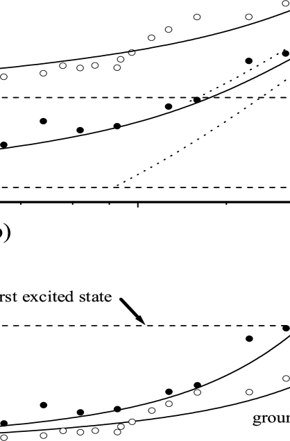
Figure 10: (a) The axial expansion of the condensate after 15 ms of free expansion for various trap geometries and atom numbers. Solid lines indicate theoretical variational predictions, dashed lines indicate the ideal gas limit and dotted lines the hydrodynamic limit. The data are taken for traps with $\omega_{z}/2\pi=1990$ Hz (open circles) and 960 Hz (filled circles). The atom numbers are $8\times 10^{4}$ and $1.1\times 10^{5}$, respectively. (b) The release energy of the condensate derived from the expansion measurements in (a). The energy tends towards the vertical zero-point kinetic energy as $\omega_{x}$ is reduced.