Analytic continuation of QMC data with a sign problem

Abstract

We present a Maximum Entropy method (MEM) for obtaining dynamical spectra from Quantum Monte Carlo data which have a sign problem. By relating the sign fluctuations to the norm of the spectra, our method properly treats the correlations between the measured quantities and the sign. The method greatly improves the quality and the resolution of the spectra, enabling it to produce good spectra even for poorly conditioned data where standard MEM fails.

I Introduction

One of the greatest advantages of Quantum Monte Carlo (QMC) simulations is the possibility to deal with complex and large size systems. The tremendous increase in computing capabilities and the development of new QMC based algorithms in recent years gives rise to new opportunities for QMC simulations. However, the possibility of producing new data implies a series of new problems for processing and analyzing the data.

Despite the QMC successes, these simulations have some general limitations. One such difficulty is the sign problem, which affects a large class of quantum models and appears when the sampling weight of some configurations is not positive definite. Another drawback of QMC simulations is that, while static measurements are easily obtained, calculating dynamical quantities is extremely difficult. When the sign problem is present, this difficulty is much more serious. In the past, the limited computing capabilities available didn’t allow for simulations with a small average sign. With the advent of new parallel vector machines such as the CRAY X1 at ORNL however, the speed of these calculations is significantly improved, making simulations with a small average sign feasible. This necessitates major improvements in the methods used to analyze the new data.

The standard technique of extracting dynamical spectra from QMC simulations based on the Matsubara-time path integral formalism is the Maximum Entropy Method (MEM) mem ; mem1 ; mem2 ; mem3 . The dynamical properties contain important information about excited states and describe the system’s response to different external perturbations, making the direct connection between model and experiment. Therefore an algorithm able to produce dynamical quantities is of crucial importance. The goal of this paper is to describe an improved MEM technique of calculating dynamical properties of a system from QMC data with a sign problem.

MEM recasts the problem of spectra calculation from a deterministic problem to one of probability optimization. In principle, by knowing the imaginary time response functions, the dynamical spectra can be obtained by solving an integral equation. However, in practice, the calculation of spectra is an ill-defined problem. Due to the fact that QMC provides information on a finite number of time points with a certain error bar, an infinite number of solutions consistent with the data exists. MEM is an algorithm which, based on Bayesian inference bayesian , provides the most probable spectrum compatible with the available data membay .

The spectrum probability is calculated assuming Gaussianly distributed and uncorrelated data. As the central limit theorem requires, the statistics of any average is Gaussian as long as the average is taken over a large number of uncorrelated points. Methods have been developed to reduce the correlations in the data, both those between adjacent measurements and those at different Matsubara time points in the same measurement mem .

However, when the sign problem is present, the QMC data becomes very poorly conditioned, which greatly complicates the MEM problem. Non-Gaussian distributions and strong correlations of the data turn out to be very severe problems. They cannot be removed by the standard techniques, mainly due to the strong correlation between the data and the averaged sign of the configurations which produce these data. This makes it essentially impossible to calculate spectra long before the minus sign problem makes the calculation of static properties impractical. In this paper we address this problem and describe a solution which greatly increases the resolution of MEM when calculating spectra from such poorly conditioned data.

This paper is organized as follows. In Sec. II we introduce the general MEM formalism. In Sec. III we discuss and exemplify the problems which appear when the QMC simulations suffer by the sign problem. A solution to the problem is given in Sec. IV. A comparison of spectra obtained with the standard and the improved method is presented in Sec. V. The conclusions are given in Sec. VI.

II MEM Formalism

We start with a brief introduction of MEMmem . MEM is an algorithm which aims to determine the spectral decomposition of one- or two-particle Green’s functions. Most QMC methods only produce estimates of the imaginary time Green’s functions. The relation between the spectral density, $A(\omega)$, and the imaginary time Green’s function, $G(\tau)$, is given by an integral equation textbooks

$$G(\tau)=\int K(\tau,\omega)A(\omega)d\omega$$ (1)

where the kernel, $K(\tau,\omega)$, is given by

$$K(\tau,\omega)=\frac{e^{-\tau\omega}}{1+e^{-\beta\omega}}$$ (2)

for the one-particle Green’s function, and respectively

$$K(\tau,\omega)=\frac{1}{\pi}\frac{\omega e^{-\tau\omega}}{1-e^{-\beta\omega}}$$ (3)

for the two-particle susceptibility .

The determination of the spectrum is an ill-posed problem, since an infinite number of solutions exists which are consistent with the QMC data and associated error bars. MEM selects from these solutions the most probable one. According to Bayesian logic bayesian , given the data $G$, the conditional probability of the spectrum $A$, $P[A|G]$, is given by

$$P[A|G]=P[G|A]~{}P[A]/P[G]\,.$$ (4)

Here $P[G|A]$ is the likelihood function which represents the conditional probability of the data $G$ given $A$, $P[A]$ is the prior probability which contains prior information about $A$ and $P[G]$ is called the evidence and can be considered a normalization constant.

The prior probability is given by

$$P[A]=e^{\alpha S},$$ (5)

with a real positive constant $\alpha$ and the entropy function $S$ defined by

$$S=\int d\omega(A(\omega)-m(\omega)-A(\omega)\ln[A(\omega)/m(\omega)]).$$ (6)

$m(\omega)$ is a function called “default model”. The specific form of the entropy function is a result of some general and reasonable assumption imposed on the spectrum, like subset independence, coordinate invariance, system independence and scaling. By defining the entropy relative to a default model, the prior probability is also used to incorporate prior knowledge about the spectrum, such as the high-frequency behavior and certain sum-rules. In the absence of data the resultant spectrum will be identical to the model. The entropic probability and its consequences are discussed at large in a series of papers entropy1 ; entropy2 ; entropy3 ; kangaroo ; mem , and does not constitute the subject of this study.

The main focus of this investigation is the calculation of the likelihood function, $P[G|A]$. The central limit theorem shows that the distribution of the data obtained in a QMC process is always Gaussian if every data point is taken as an average of a large enough number of measurements so that different data are independent. This implies

$$P[G|A]=e^{-\chi^{2}/2}$$ (7)

where

$$\chi^{2}=\sum^{L}_{i,j=1}(\bar{G}_{i}-G_{i}(A))[C^{-1}]_{ij}(\bar{G}_{j}-G_{j}(A)),$$ (8)

$$\bar{G}_{i}=\frac{1}{M}\sum^{M}_{m=1}G^{(m)}_{i}$$ (9)

with the covariance

$$C_{ij}=\frac{1}{M-1}\sum^{M}_{m=1}(\bar{G}_{i}-G^{(m)}_{i})(\bar{G}_{j}-G^{(m)}_{j}).$$ (10)

Here we considered that QMC provides $G(\tau)$ on $L$ time points $\tau_{i}$, and denote $G(\tau_{i})\equiv G_{i}$. For every time point, $\tau_{i}$, we have $M$ measured $G^{(m)}_{i}$, centered at $\bar{G}_{i}$ (Eq. 9). $C$ in Eq. (10) is the covariance matrix which characterizes the second moment of the data. $G_{i}(A)$ in Eq. (8) is the value of $G(\tau_{i})$ which corresponds to the spectrum $A(\omega)$ according to Eq. 1 or its discretized form.

MEM requires Gaussianly distributed data. Otherwise, the likelihood probability defined in Eq. (7) has no meaning. In theory, the requirement for a Gaussian distribution is achieved by averaging many measurements to obtain one data point. However, in practice when computational resources are limited, this condition is often difficult to satisfy. In MEM literature the data points obtained by averaging many measurements are called bins. The usual way to remove the correlation between bins is to re-average (coarse-grain) more successive bins which results in increasing the number of measurements per bin. However, for a fixed amount of data, this process of increasing the bin size will reduce the number of data points (bins). If the number of bins is too small, the data cannot properly describe a statistic process, and the covariance matrix becomes pathological. Therefore a successful MEM for correlated data requires a large number of measurements, implying both large bins and a large number of bins.

The correlation of data between different time points, is the other relevant problem which causes MEM to fail. These correlations can be removed by a rotation $U$ which diagonalizes the covariance matrix.

$$C^{\prime}_{ij}=(U^{-1}CU)_{ij}=\sigma^{2}_{i}\delta_{ij}.$$ (11)

The data and the kernel should also be rotated accordingly

$$K^{\prime}=U^{-1}K,~{}~{}~{}~{}G^{\prime}=U^{-1}G$$ (12)

The rotated $G^{\prime}_{i}$ are the statistically independent directions, and in this basis, $\chi^{2}$ reduces to

$$\chi^{2}=\sum^{L}_{i=1}\frac{(\bar{G^{\prime}}_{i}-\sum^{N_{f}}_{\nu=1}K^{\prime}_{i\nu}A_{\nu})^{2}}{\sigma^{2}_{i}}.$$ (13)

In Eq. 13 the discretized form of Eq. 1 was used, the summation over $\nu$ meaning summation over frequency.

III Data produced by QMC simulations with sign problem

Figure 1: Histogram of the distribution of a) $Gs(\beta/16)$, b) sign, $s$ and c) $G(\beta/16)$ when the bin size is increased five times which corresponds to $3000$ measurements per bin. The dashed lines represent the best Gaussian fit to the data.

When the sign problem is present in QMC simulations, the condition of Gaussianly distributed $G_{i}$ becomes more difficult to satisfy. Very often, a huge number of measurements, beyond the available computing possibilities, would be required to accomplish this task.

The difficulty in obtaining good data points for $G_{i}$ can be easily understood from the measurement process. In a QMC process where the sign of the sampling weight is negative, it can no longer define a probability. Therefore, the sign of the sampling weight must be associated with the measurement. For the Green’s function, we can no longer measure $G_{i}$ but rather the product of it and the sign $s$ of the configuration, $Gs_{i}\equiv G_{i}*s$, and the sign $s$. At the end of the simulation, i.e. after a large number of measurements, we then obtain $\bar{G}_{i}=\overline{Gs_{i}}/\bar{s}$, where the overbar denotes averaging over the number of measurements. Two problems related with the sign affect the quality of the $G_{i}$ data. First, in order to obtain good data points $G_{i}^{(m)}$, for every data point we need to average a very large number of $Gs_{i}$ and $s$ and afterwards calculate $G_{i}^{(m)}=Gs_{i}^{(m)}/s^{(m)}$. Here $Gs_{i}^{(m)}$ and $s^{(m)}$ both denote averages over the measurements that form the bin $m$. Smaller average signs $\bar{s}$ worsen the problem, since any small variation of $s$ has a large effect on $G_{i}$ ($\propto 1/\bar{s}^{2}$). Second, as within the same bin $m$ there is a strong correlation between different data points $Gs_{i}^{(m)}$, there is also a strong correlation between data points $Gs_{i}^{(m)}$ and $s^{(m)}$. The points $G_{i}^{(m)}=Gs_{i}^{(m)}/s^{(m)}$ are obtained by a nonlinear operation of these correlated quantities, and there is no reason to expect them to be normal distributed.

In order to exemplify the problems discussed above, we employed a QMC based algorithm dca to produce a very large amount of data for the single-particle Green’s function and the two-particle spin susceptibility in the two-dimensional Hubbard model on a square lattice. The Hubbard model is characterized by the single-particle hopping $t$ between nearest neighbors and the on-site Coulomb repulsion $U$. We choose $t=0.25$ so that the bandwidth $W=2$ and set $U=W$. To make the sign-problem worse, we add a next-nearest neighbor hopping $t^{\prime}=-0.3t$ to frustrate the lattice. We perform calculations on a 16-site $4\times 4$ cluster at $15\%$ doping, down to temperatures $T=0.125t$ where we experience a severe sign-problem, $\bar{s}=0.051$. We simulate the model using the dynamical cluster approximation (DCA) with the Hirsch-Fye algorithm as a cluster solver.dca The DCA is a coarse-graining approximation, in which the one particle Green’s function is coarse-grained in the first Brillouin zone of the reciprocal space of the lattice. It is defined over cluster points $K=(K_{x},K_{y})$ and imaginary time $\tau$, and accurately describes short-ranged correlations. We performed the simulations on the Cray $X_{1}$ supercomputer at Oak Ridge National Laboratory to cope with the large amount of data needed in simulations with small average signs. We calculated $8000$ data points (bins) $(Gs_{i}^{(m)},s^{(m)})$, and for every data point we averaged $600$ QMC measurements.

In Fig. 1 we show histograms of the data distribution when the bin size is increased five times, which corresponds to an average of $3000$ measurements per bin. Both $Gs(\beta/16)$ (Fig. 1 (a)) and $s$ (Fig. 1 (b)) are normally distributed to a good approximation, unlike $G(\beta/16)$ data points (Fig. 1 (c)) which are strongly peaked, being characterized by a large positive kurtosis kurt . Similar distributions of data are observed (not shown) for the other values of the imaginary time. In order to become Gaussianly distributed the $G$ data require averaging over a much larger number of measurements than $Gs$ and $s$ data. In our case this number is about five times larger but this value is dependent on the specificity of the problem considered, being determined by both the magnitude of the correlations and the value and the distribution of the sign .

The way to achieve good data for MEM is i) rebinning $(Gs_{i},s)$ until they become normal distributed, and ii) remove the correlations between data points $Gs_{i}$ and $s$ by a rotations in the space $(Gs_{i},s)$. However, the problem that arises is the calculation of $\chi^{2}$ (Eq. 8, 13) in this basis which now includes the extra sign dimension. This issue will be discussed in the next section (Sec. IV).

IV Likelihood function

IV.1 Formalism

Denoting $h\equiv(Gs,s)$, the likelihood function is defined as $P[h|A]$, since the measured quantities in the QMC process are the $h$ points (and not $G$). As we showed in the previous section, for acceptable values of the bin size, the data $h$ are to a good approximation Gaussianly distributed. Therefore, the likelihood function will have the same form as Eq. 7, with $\chi^{2}$

$$\chi^{2}=\sum^{L+1}_{i,j=1}(\bar{h}_{i}-h_{i}(A))[C_{h}^{-1}]_{ij}(\bar{h}_{j}-h_{j}(A))\,.$$ (14)

The covariance matrix has now the dimension $(L+1)\times(L+1)$,

$${C_{h}}_{ij}=\frac{1}{M-1}\sum^{M}_{m=1}(\bar{h}_{i}-h^{(m)}_{i})(\bar{h}_{j}-h^{(m)}_{j}).$$ (15)

The only problem which remains to be solved is finding an equation for $h(A)$, since Eq. 1 only provides a relation for $G(A)$. In order to achieve this we do the following: First we absorb the sign into the spectrum, i.e. we define ${\cal{A}}$ as

$${\cal{A}}(\omega)=sA(\omega)~{}.$$ (16)

Instead of searching for a spectrum $A$ which satisfies Eq. 1 we search for ${\cal{A}}$ which satisfies

$$Gs(\tau)=\int K(\tau,\omega){\cal{A}}(\omega)d\omega~{}.$$ (17)

Second, we consider the spectrum normalization sum-rule

$$B=\int A(\omega)d\omega,$$ (18)

which implies

$$s=\int\frac{1}{B}{\cal{A}}(\omega)d\omega~{}.$$ (19)

Here $B$ is a constant, equal to one for the the one-particle spectra and equal to $\chi(T)$ for the two-particle case . Because the sign $s$ was absorbed into the definition of ${\cal{A}}$ we relate the sign fluctuations to the norm of the new spectrum. Both Eq. 17 and Eq. 19 can be written as

$$\bar{h}_{i}=\sum_{\nu=1}^{N_{f}}{K_{h}}_{i\nu}{\cal{A}}_{\nu},~{}~{}~{}{K_{h}}_{i\nu}=\left\{\begin{array}[]{ll}{K}_{i\nu}&~{}i\leq L\\ \frac{1}{B}&~{}i=L+1\\ \end{array}\right.~{}~{}.$$ (20)

This is the basic equation which relates $h$ to ${\cal{A}}$ and determines the likelihood function $P[h|A]\equiv P[h|{\cal{A}}]$. MEM will produce the most probable spectrum ${\cal{A}}$ normalized to $\bar{s}$ which minimizes the $\chi^{2}$ function in Eq. (14) subject to the entropy constraint.

IV.2 Discussion

We want to point that for the one-particle case, where $B=1$, Eq. (19) is equivalent to

$$Gs(0)+Gs(\beta)=s~{}.$$ (21)

By using Eq. (19) in the calculation of the likelihood function we impose

$$G(0)+G(\beta)=\frac{Gs(0)}{s}+\frac{Gs(\beta)}{s}=1,$$ (22)

at every measurement. Since Eq. 22 results solely from the anticommutation relation of the one-particle operators it should be satisfied in every possible configuration and implicitly in every measurement. Therefore, this way of implementing the normalization sum-rule is more natural than the usual way based on Lagrange multipliers where the constraint is globally imposed, i.e. not at every measurement but only for the final Green’s function obtained at the end of the QMC process.

For the two-particle case, where $B=\chi(T)$, the sum-rule Eq. (18) is not an independent equation as in the one-particle case, but merely an integration over $\tau$ of Eq. 1. Therefore it is essential to treat $B$ as a constant (equal to the final, averaged over all QMC configurations, $\bar{\chi}(T)$) and to disregard measurement dependent fluctuations in $\chi(T)$. This way we relate the norm of ${\cal{A}}$ only to the fluctuation of the sign $s$.

V Comparison of the spectra obtained with the two methods

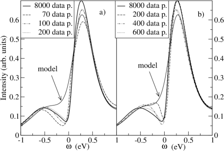
Figure 2: One-particle spectra at $K=(\pi,\pi/2)$ calculated with different amounts of data using a) the new method and b) the old method.

In this section we present a comparison between the spectra obtained with the old approach which does not consider the sign covariance, and the new one described in Sec. IV. For calculating the one-particle spectrum at the highest temperatures, the model $m(\omega)$ used in the entropy functional Eq. (6), is chosen to be a Gaussian function. The model for lower temperatures is taken to be the spectrum obtained at a slightly higher temperature, a procedure called annealing.

In Fig. 2 (a) and (b) we show the one-particle spectra of the Hubbard model at $K=(\pi,\pi/2)$ calculated for different amounts of data with the new and respectively with the old method. In both cases, when a large amount of data is used ($8000$ data points) the spectrum (thick continuous line) is converged. Moreover the two methods produce the same spectrum. However, it can be noticed that with the new method a reasonably good spectrum, i.e. a spectrum close to the converged one, can be obtained with an amount of data as small as $100$ data points (see the double-dotted dashed line in Fig. 2 (a)). On the other hand, the old method requires at least $600$ data points for a spectrum of comparable quality (see the dotted line in Fig. 2 (b)). Thus in our case we find that the new method reduces the computational cost of calculating the one-particle spectra about six times.

In general the calculation of the two-particle spectra turns out to be more difficult, because the data are more correlated and because a good default model is missing. In our case the amount of data needed for calculating the two-particle spectra is about one order of magnitude larger. At high temperature we choose a default model of the form

$$m(\omega)=\exp[\lambda_{0}+\lambda_{1}\omega\coth(\beta\omega/2)]$$ (23)

where $\lambda_{0}$ and $\lambda_{1}$ are Lagrange multipliers chosen to satisfy certain moment constraints, as described in ref mem . Again, the annealing technique is used for lower temperature calculations.

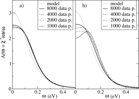
Figure 3: Two-particle spin susceptibility spectra $A(\omega)=\chi^{\prime\prime}(\omega)/\omega$ at $K=(0,\pi/2)$ calculated for different amounts of data with a) the new method and b) the old method.

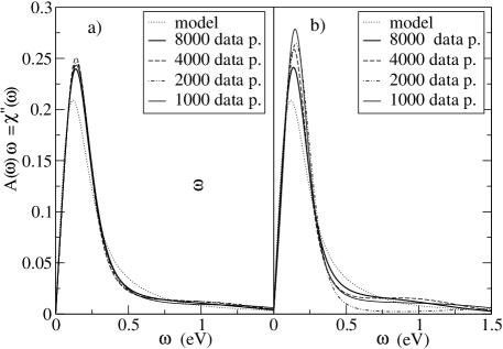
Figure 4: Imaginary part of the spin susceptibility $\chi^{\prime\prime}(\omega)=A(\omega)\omega$ at $K=(0,\pi/2)$ calculated for different amount of data with a) the new method and b) the old method.

The spin susceptibility spectra at $K=(0,\pi/2)$ calculated with the two methods for different amounts of data is shown in Fig. 3. For the two-particle case the spectra $A(K,\omega)$ defined in Eq. 1 is in fact $\chi^{\prime\prime}(K,\omega)/\omega$ where $\chi^{\prime\prime}(K,\omega)$ is the imaginary part of the spin susceptibility. When a large amount of data is used ($8000$ data points) both methods produce the same spectrum (thick continuous line in both Fig. 3 (a) and (b)). However, for small amounts of data, the new method produces significantly superior results to the old method. For example the spectrum obtained with the new method for $1000$ data points (thin continuous line in Fig. 3 (a)) is closer to the converged spectrum than the one obtained with the old method for $4000$ data points (dashed line in Fig. 3 (b)). The same conclusion can be drawn by comparing the high energy features ($\approx 0.5-1.5~{}eV$) visible in the plot of the imaginary part of the spin susceptibility $\chi^{\prime\prime}(K,\omega)$ in Fig. 4 (a) and (b).

VI Conclusions

We showed that for QMC simulations with a severe sign problem, achieving a normal distribution of $G$ is extremely difficult. The problem results from the nonlinear operation which relates $G$ to the measured quantities $Gs$ and $s$, and from the correlation between the $Gs$ points and $s$.

By absorbing the sign into the definition of the spectrum, the sign fluctuations will determine the norm of the spectrum. A connection is thus established between the measured quantities $(Gs,s)$ and the renormalized spectrum ${\cal{A}}=As$. The likelihood function is calculated with regard to the directly measured $(Gs,s)$ data, thus no nonlinear manipulation of the data is being applied. The correlations between $Gs$ and $s$ can be removed by a rotation in the space determined by these vectors.

We illustrated the power of this approach by a comparison of the spectra obtained with the old and the new method. When the sign is small and the correlation between the sign $s$ and the measured $Gs$ points is significant, the old method requires a very large amount of measurements per bin in order to produce the normally distributed and uncorrelated data points necessary for obtaining good spectra. In contrast, the new method provides good spectra for a much smaller amount of data. In our case the old method needs about six times more data than the new one, but for other problems characterized by stronger correlations this amount can be much larger.

References

- (1) R. N. Silver, D. S. Sivia and J.E. Gubernatis, Phys. Rev. B 41, 2380 (1990)
- (2) R. N. Silver, J. E. Gubernatis, D. S. Sivia, and M. Jarrell, Phys. Rev. Lett. 65, 496 (1990)
- (3) J. E. Gubernatis, M. Jarrell, R. N. Silver and D. S. Sivia, Phys. Rev. B 44, 6011 (1991)
- (4) Mark Jarrell and J. E. Gubernatis, Physics Reports 269, 133, (1996)
- (5) A. Papoulis, Probability and Statistics(Prentice-Hall, New York, 1990), p. 422
- (6) E. T. Jaynes, in Maximum Entropy and Bayesian Methods edited by J. H. Justice (Cambridge University, Cambridge, 1986); S.F. Gull in Maximum Entropy and Bayesian Methods in Science and Engineering, edited by G. J. Erickson and C. R. Smith (Kluwer Academic, Dordrecht, 1988) D.S. Sivia, Los Alamos Science 19, 180, (1990)
- (7) S. Doniach and E. Sondheimer Green’s Functions for Solid State Physicists (Benjamin, Reading, MA, 1974); R. Kubo, M. Toda and N. Hashitsume, Statistical Physics II (Springer-Verlag, New York, 1978); S. W. Lovesoy, Condensed Matter Physics (Benjamin/Cummings, Reading, MA, 1980); G. D. Mahan, Many Particle physics (Kluwer Academic/Plenum New York, 2000).
- (8) J. Skilling in Maximum Entropy and Bayesian Methods edited by J. Skilling (Kluwer Academic, Dordrecht, 1989), p.45
- (9) S.F Gull in Maximum Entropy and Bayesian Methods edited by J. Skilling (Kluwer Academic, Dordrecht, 1989), p.53
- (10) R.K. Bryan, Eur. Biophys. J. 18, 165, (1990)
- (11) S. F. Gull and J. Skilling, IEE Proceedings 131, 646 (1984)
- (12) M. Jarrell, Th. Maier, C. Huscroft and S. Moukouri, Phys. Rev. B. 64 195130 (2001)
- (13) W.H. Press, S.A. Teukolsky, W.T. Vettering and B.P. Flannery Numerical Recipes (Cambridge University Press, 1989), chap. 14