Exactly-solvable problems for two-dimensional excitons

Abstract

Several problems in mathematical physics relating to excitons in two dimensions are considered. First, a fascinating numerical result from a theoretical treatment of screened excitons stimulates a re-evaluation of the familiar two-dimensional hydrogen atom. Formulating the latter problem in momentum space leads to a new integral relation in terms of special functions, and fresh insights into the dynamical symmetry of the system are also obtained. A discussion of an alternative potential to model screened excitons is given, and the variable phase method is used to compare bound-state energies and scattering phase shifts for this potential with those obtained using the two-dimensional analogue of the Yukawa potential. The second problem relates to excitons in a quantising magnetic field in the fractional quantum Hall regime. An exciton against the background of an incompressible quantum liquid is modelled as a few-particle neutral composite consisting of a positively-charged hole and several quasielectrons with fractional negative charge. A complete set of exciton basis functions is derived, and these functions are classified using a result from the theory of partitions. Some exact results are obtained for this complex few-particle problem.

Introduction

Dimensionality plays an important role in condensed matter physics, with many fascinating new phenomena emerging as the number of dimensions is reduced. With the introduction of improved semiconductor growth techniques over the past few decades, physical realisation of these systems has become possible.

One of these systems is a quantum well, fabricated by sandwiching a layer of semiconductor between two layers of another material with a higher bandgap. The motion of electrons and holes is ‘frozen’ in the growth direction, and in modelling the system we may consider the electrons and holes as being essentially confined to a plane. As in bulk semiconductors, the Coulomb interaction between electrons and holes leads to bound states, known as excitons, which are extremely important for the optical properties of the quantum well.

The introduction of a strong magnetic field in the growth direction leads to further interesting phenomena in two-dimensional systems. At sufficiently low temperatures, many-electron correlations become important and new states of matter are formed. One of these states of matter is an incompressible quantum liquid, whose excitations carry fractional charge and obey fractional statistics. Spectroscopic techniques can be used to probe the properties of such systems, and excitonic effects are again of the utmost importance.

This Chapter will focus on a diverse range of problems in mathematical physics which have arisen as a result of our work on the theory of excitons in semiconductor nanostructures. The areas covered include the theory of special functions, dynamical symmetries in quantum mechanics, symmetric polynomials, the theory of partitions and counting of bound states in short-range potentials.

In Section 1 we discuss a fascinating numerical result that arisies from a theoretical treatment of screened excitons. This stimulates a re-evaluation of the familiar two-dimensional hydrogen atom. Formulating the latter problem in momentum space leads to a new integral relation in terms of special functions, and fresh insights into the dynamical symmetry of the problem are also obtained. A discussion of an alternative potential to model screened excitons is given, and bound-state energies and scattering phase shifts for this potential are compared with those obtained using the two-dimensional analogue of the Yukawa potential.

In Section 2 we consider an exciton consisting of a valence hole and several fractionally-charged quasielectrons (anyons). A complete set of basis functions is obtained for this ‘anyon exciton’ and these functions are classified using a result from the theory of partitions. Expressions are derived for the overlap and interaction matrix elements of four- and six-particle systems, which describe an exciton against the background of incompressible quantum liquids with filling factors 1/3, 2/3 and 2/5. Some exact results are obtained for the general $(N+1)$-particle case, including the binding energy for an exciton with zero in-plane momentum and zero internal angular momentum.

1 Two-dimensional exciton: screened and unscreened

1.1 Motivation

Modelling of a screened Wannier-Mott exciton in two dimensions using the Stern-Howard potential [1] has revealed an intriguing numerical relation [2, 3]. In the search for an analytical derivation of this result, we address the simpler problem of an unscreened two-dimensional (2D) exciton, which has a well-known solution in real space. It has been claimed that the aforementioned numerical relation is not strictly exact, and an alternative approach to the problem has been proposed [4]. This has led to a new potential for modelling screened excitons, which is also considered here.

1.2 Screened 2D Wannier-Mott exciton

Illumination of a semiconductor with near-bandgap light leads to the creation of electron-hole bound states known as excitons. The study of excitons in condensed matter physics has a long history [5]. Broadly speaking, excitons can be divided into two types: hydrogen atom-like Wannier-Mott excitons and more tightly-bound Frenkel excitons. In the present work we shall only be concerned with the first of these.

Advances in semiconductor growth techniques have led to the creation of almost ideal 2D systems. In such systems, confinement leads to a higher exciton binding energy than in the bulk, which makes 2D excitons more experimentally accessible. A semiconductor quantum well is a quasi-two-dimensional system, in which photoexcited electrons and holes are essentially confined to a plane as their motion is ‘frozen’ in the growth direction. Excitons are extremely important for the optical properties of the quantum well. If enough electrons and holes are excited, the Coulomb attraction between particles may be weakened - this phenomenon is known as screening. The effect of screening on an exciton may be approximated by considering the electron and hole as interacting via the so-called Stern-Howard potential [1], which has the following form in real space:

$$V_{s}(\rho)=-\frac{2}{\rho}\left\{1-\frac{\pi}{2}q_{s}\rho\left[\mathbf{H}_{0}(q_{s}\rho)-N_{0}(q_{s}\rho)\right]\right\}=-\frac{2}{\rho}\left\{1-q_{s}\rho\,S_{0,0}(q_{s}\rho)\right\},\vspace{3mm}$$ (1)

where $q_{s}$ is known as the 2D screening wavenumber, and $\mathbf{H}_{0}$, $N_{0}$ and $S_{0,0}$ are the Struve, Neumann and Lommel functions, respectively. Note that all lengths and energies are measured in units of three-dimensional (3D) exciton Bohr radius and excitonic Rydberg, respectively. In these units, the radial equation for the relative electron-hole motion is given by

$$-\frac{d^{2}R(\rho)}{d\rho^{2}}-\frac{1}{\rho}\frac{dR(\rho)}{d\rho}+\left(V_{s}(\rho)+\frac{m^{2}}{\rho^{2}}\right)R(\rho)=ER(\rho).\vspace{3mm}$$ (2)

This is the radial part of the 2D Schrödinger equation, which is discussed in more detail in Sections 1.6 and 3.1. In Eq. (2), $m$ is the azimuthal quantum number, which takes integer values.

Numerical calculations [2, 3] using Eq. (1) have shown that with increasing screening, bound states in this potential disappear at integer values of the inverse screening wavenumber $1/q_{s}$. This ‘empirical’ observation can be formulated as the following Sturm-Liouville problem:

$$\left(\hat{A}-\frac{m^{2}}{x^{2}}\right)F(x)+\lambda V(x)F(x)=0,\vspace{3mm}$$ (3)

where

$$\hat{A}=\frac{1}{x}\frac{d}{dx}x\frac{d}{dx},\vspace{3mm}$$ (4)

$\lambda=2/q_{s}$, and we have made the substitution $x=q_{s}\rho$. The zero right-hand side of Eq. (3) reflects the fact that we restrict our interest to zero-energy bound states. The function $V(x)$ is defined as

$$V(x)=\frac{1}{x}-S_{0,0}(x),\vspace{3mm}$$ (5)

and it has the following properties:

$$\int_{0}^{\infty}V(x)\,x\,dx=1\quad\mbox{and}\quad V(x)=\hat{A}\left\{\frac{1}{x}-V(x)\right\}.\vspace{3mm}$$ (6)

The key result of [2] is that the solution $F$ of Eq. (3) is square-integrable, i.e.

$$\int_{0}^{\infty}|F(x)|^{2}\,x\,dx=1,\vspace{3mm}$$ (7)

only if

$$\lambda=(2|m|+\nu)(2|m|+\nu+1),\vspace{3mm}$$ (8)

where $\nu=0,1,2,\ldots$ is the number of non-zero nodes in the radial wavefunction.

Notably, the potential defined in Eq. (1) is simplified considerably if we move to Fourier space:

$$V_{s}(q)=-\frac{4\pi}{\left(q+q_{s}\right)}.\vspace{3mm}$$ (9)

Eq. (9) is the 2D analogue of the familiar Yukawa potential (a standard textbook derivation for both the 2D and 3D cases can be found in [6], for example).

The most compact way to reformulate the above Sturm-Liouville problem is in terms of a homogeneous integral equation:

$$q^{2}\Phi(\mathbf{q})=\frac{\lambda}{2\pi}\int\frac{\Phi(\mathbf{q^{\prime}})}{|\mathbf{q}-\mathbf{q^{\prime}}|+1}\,d^{2}q^{\prime}.\vspace{3mm}$$ (10)

It follows that $\Phi(\mathbf{q})$ is square-integrable in 2D Fourier space when $\lambda$ satisfies Eq. (8). It should be emphasised that this result is of a numerical nature and has not been proved analytically.

In an attempt to find an analytical derivation of Eq. (8) we address the simpler problem of an unscreened 2D exciton. This system is analogous to the 2D hydrogen atom, with the proton replaced by a valence hole, so we now focus our attention on such a system.

1.3 Hydrogen atom and accidental degeneracy

The in-plane motion of an electron and hole can be described by a two-dimensional Schrödinger equation for a single particle with a reduced mass. As in three dimensions, the 2D hydrogen atom exhibits ‘accidental’ degeneracy of the bound-state energy levels.

Before proceeding it is necessary to discuss accidental degeneracy in more detail. The phenomenon of accidental degeneracy is well known from the theory of the 3D hydrogen atom. There are three quantum numbers $\{n,l,m\}$, although the energy only depends on the principal quantum number $n$.

Degeneracy in $m$ is of geometrical origin, and is due to the invariance of the system under spatial rotations. From Noether’s theorem [7], this symmetry implies the existence of a conserved quantity, which is the angular momentum $\hat{\mathbf{L}}$. Indeed, quantum mechanics tells us that whenever there is a conserved quantity whose components cannot be measured simultaneously, then the energy eigenvalues will be degenerate [8].

The origin of the degeneracy in $l$, however, is not so obvious. In fact, this degeneracy does not have a geometrical origin, but arises from a hidden dynamical symmetry of the system. The conserved quantity associated with this accidental degeneracy is the Runge-Lenz vector $\hat{\mathbf{A}}$, the components of which cannot be measured simultaneously. The existence of the Runge-Lenz vector is not so well known because when the Schrödinger equation is separated in spherical polar coordinates, the natural choice for a complete set of commuting operators is $\{\hat{H},\hat{L}_{z},\hat{L}^{2}\}$, where $\hat{H}$ is the Hamiltonian. However, the presence of the Runge-Lenz vector is evident if the Schrödinger equation is separated in parabolic coordinates, as the natural choice for a complete set of commuting operators is then $\{\hat{H},\hat{L}_{z},\hat{A}_{z}\}$. In general, accidental degeneracy appears when the Schrödinger equation can be separated in more than one coordinate system (for a detailed review see [9]).

In two dimensions there are two quantum numbers $\{n,m\}$. However, the energy eigenvalues only depend on $n$, so they are degenerate in the quantum number $m$. In this case the angular momentum only has a $z$-component (where $z$ is in the direction perpendicular to the plane of motion), and so it can be known precisely. The degeneracy in $m$ is therefore due to the existence of a 2D Runge-Lenz vector and a corresponding dynamical symmetry of the system.

1.4 Historical background

The Runge-Lenz vector has its origin in classical mechanics (see Fig. 1), and its discovery has been variously attributed to Laplace, Runge, Lenz and Hamilton (see [10] and references therein).

Figure 1: Classical Runge-Lenz vector A.

A result known as Bertrand’s theorem states that the only central forces which result in closed orbits are the inverse square law (Kepler problem) and Hooke’s law [10, 11]. The closure of orbits is due to the conservation of an additional quantity (apart from the energy and angular momentum); in the case of the Kepler problem this quantity is the Runge-Lenz vector

$$\mathbf{A}=\frac{1}{\mu}\left(\mathbf{p}\times\mathbf{L}\right)-\kappa\frac{\mathbf{r}}{r},\vspace{3mm}$$ (11)

where $\mu$ is the reduced mass, $\mathbf{p}$ is the momentum, $\mathbf{L}$ is the angular momentum, $\kappa$ is a positive constant and $\mathbf{r}$ is the radius vector of the orbit.

A quantum mechanical analogue of the Runge-Lenz vector was first suggested by Pauli [12], by analogy with classical mechanics. The main difference is that it is now an operator:

$$\hat{\mathbf{A}}=\frac{1}{2\mu}\left(\hat{\mathbf{p}}\times\hat{\mathbf{L}}-\hat{\mathbf{L}}\times\hat{\mathbf{p}}\right)-\kappa\frac{\hat{\mathbf{r}}}{r},\vspace{3mm}$$ (12)

where the form of the first term on the right-hand side ensures that $\hat{\mathbf{A}}$ is Hermitian. Pauli also made the key conclusion that the existence of a Runge-Lenz vector constant in time implies that the hydrogen atom exhibits an additional degeneracy to that due to conservation of angular momentum. He then used $\hat{\mathbf{A}}$ to derive the correct energy levels for the hydrogen atom.

The most important paper concerning the symmetry of the hydrogen atom was published by Fock in 1935 [13]. His first step was to consider the Schrödinger equation in momentum space, which resulted in an integral equation. Considering only negative energy (bound-state) solutions, he then projected the 3D momentum space onto the surface of a four-dimensional (4D) hypersphere using a stereographic projection. After a suitable transformation of the wavefunction, the resulting Schrödinger equation is seen to be invariant under rotations in 4D Euclidean space. The kernel is just the Green’s function of Laplace’s equation in four dimensions. Application of Green’s theorem yields the correct energy eigenvalues, as well as eigenfunctions in terms of hyperspherical harmonics. Fock deduced that the dynamical symmetry of the hydrogen atom is described by the 4D rotation group SO(4), which contains the geometrical symmetry SO(3) as a subgroup. He related this hidden symmetry to the observed degeneracy of the energy eigenvalues.

Shortly afterwards, Bargmann [14] made the connection between Pauli’s quantum mechanical Runge-Lenz vector and Fock’s discovery of invariance under rotations in 4D space. The real-space Schrödinger equation was also separated in parabolic coordinates, which demonstrated more explicitly the conservation of the Runge-Lenz vector.

A major step forward was taken by Alliluev [15], who extended Fock’s method of stereographic projection to the case of $d$ dimensions $(d\geqslant 2)$. He derived general expressions for the eigenfunctions and eigenvalues of the problem, and clarified some of Fock’s arguments relating to the symmetry group for the $d$-dimensional case. Alliluev also considered the 2D harmonic oscillator, the symmetry group of which is isomorphic to the 3D rotation group SO(3). This provided an interesting parallel to the hydrogen atom case.

The first explicit use of Fock’s method for the 2D hydrogen atom was made by Shibuya and Wulfman [16]. In this case, the eigenfunctions are just the usual spherical harmonics in three dimensions. The authors also included a graphical illustration of the degeneracy, in which two eigenfunctions which look very different on a plane are shown to be equivalent when projected onto a sphere. (It should be noted that the solution of the real-space Schrödinger equation in two dimensions was first provided in [17], although the derivation was later repeated in [18].)

In the 1960s there was a revival of interest in accidental degeneracy as it was hoped that it could be applied to the theory of elementary particles. It attracted the attention of such famous names as Gell-Mann, Schwinger and Ne’eman. In a wide-ranging study [19, 20], Bander and Itzykson provided a comprehensive review of work thus far. The first part gives a detailed explanation of the earlier work of Fock and Alliluev, the details of which are difficult to glean from the original works. Two systems of generalised spherical harmonics are then considered on the 4D hypersphere: the standard hyperspherical harmonics, and an alternative in terms of Wigner $D$-functions. These are related to separation of variables is spherical polar and parabolic coordinates, respectively. For the 3D hydrogen atom, the Runge-Lenz vector in real space is shown to correspond to the infinitesimal generator of rotations on the 4D hypersphere. A detailed group-theoretical analysis of the hydrogen atom is also given. In the second part, the analysis is extended to scattering states, where the momentum space is now projected onto a higher-dimensional hyperboloid.

The next few decades saw little progress, probably because the important questions had already been addressed so thoroughly. However, improvements in semiconductor growth techniques enabled the manufacture of effectively 2D structures, which soon led to a resurgence of interest in the 2D hydrogen atom.

In a series of papers [21, 22, 23], the 2D Runge-Lenz vector was defined for the first time, and real-space solutions of the Schrödinger equation were applied to problems of atomic physics in two dimensions, including dipole matrix elements, the Stark effect, photon transition rates and fine/hyperfine structure. The relativistic case was also considered.

Returning to higher dimensions, the use of hydrogenoid orbitals as basis sets for problems in quantum chemistry led to a re-examination of the separability of the $d$-dimensional Schrödinger equation in different coordinate systems [24]. A novel approach was taken by Nouri [25], who considered the $d$-dimensional Coulomb problem in quantum phase space. This led to an expression for the Wigner distribution function, from which it is possible to calculate some physical and chemical properties for the hydrogen atom. The dynamical symmetry of the hydrogen atom has also been related to Kac-Moody algebras, rather than the usual Lie algebras [26, 27]. This provides fertile ground for mathematical investigation and will no doubt lead to a new direction for research.

Recent studies [28, 29] have shown that the classical Runge-Lenz vector has a deeper physical origin, being tied to the generator of Lorentz transformations for the relativistic two-body problem; the non-relativistic Kepler problem is then just a zero-order description of the more general case. In principle, it should be possible to undertake a similar analysis of the quantum mechanical problem based on the Dirac equation.

Fock’s method for the 3D hydrogen atom has been applied by Muljarov et al. [30, 31] to the problem of an exciton with anisotropic mass and dielectric constant, providing an interesting alternative to a variational approach [32]. The anisotropy is considered as a perturbation, and the perturbed wavefunction is expanded in terms of the hyperspherical harmonics. Brillouin-Wigner perturbation theory is then used to calculate the energy levels and eigenfunctions of the perturbed system.

1.5 Fock’s method

We now present an outline of Fock’s approach to the 3D hydrogen atom [13], which led to important insights into the dynamical symmetry of the problem. We start from the Schrödinger equation in real space

$$\left(-\nabla^{2}-\frac{2}{r}\right)\Psi(\mathbf{r})=E\Psi(\mathbf{r}),\vspace{3mm}$$ (13)

with distances and energies measured in terms of the 3D Bohr radius $a_{0}=\hbar^{2}/\mu e^{2}$ and Rydberg $Ry=\mu e^{4}/2\hbar^{2}$, where $\mu$ is the reduced mass of the system.

Introducing the pair of Fourier transforms between real space and momentum space

$$\Phi(\mathbf{p}) =\int\Psi(\mathbf{r})e^{i\mathbf{p}\cdot\mathbf{r}}\,d\mathbf{r},$$ (14)

$$\Psi(\mathbf{r}) =\frac{1}{(2\pi)^{3}}\int\Phi(\mathbf{p})e^{-i\mathbf{p}\cdot\mathbf{r}}\,d\mathbf{p},$$ (15)

and noting that for bound states the energy $E=-p_{0}^{2}$ will be negative, we may write the Schrödinger equation as an integral equation

$$\left(p^{2}+p_{0}^{2}\right)\Phi(\mathbf{p})=\frac{1}{\pi^{2}}\int\frac{\Phi(\mathbf{p^{\prime}})\,d\mathbf{p^{\prime}}}{|\mathbf{p}-\mathbf{p^{\prime}}|^{2}}.\vspace{3mm}$$ (16)

The 3D momentum space is now projected onto the surface of a 4D unit hypersphere centred at the origin, and the in-plane momentum is scaled by $p_{0}$. A point on the hypersphere is specified by three angles, $\theta$, $\phi$ and $\alpha$, where $\alpha$ is the angle between the position vector of the point and the fourth axis introduced in the 4D space. The transformation is given explicitly by

$$u_{1} =\sin\alpha\sin\theta\cos\phi=\frac{2p_{0}p_{x}}{p^{2}+{p_{0}}^{2}},$$ (17)

$$u_{2} =\sin\alpha\sin\theta\sin\phi=\frac{2p_{0}p_{y}}{p^{2}+{p_{0}}^{2}},$$ (18)

$$u_{3} =\sin\alpha\cos\theta=\frac{2p_{0}p_{z}}{p^{2}+{p_{0}}^{2}},$$ (19)

$$u_{4} =\cos\alpha=\frac{p^{2}-{p_{0}}^{2}}{p^{2}+{p_{0}}^{2}}.$$ (20)

An element of surface area on the unit hypersphere is given by

$$d\Omega=\sin^{2}\alpha\sin\theta\,d\alpha\,d\theta\,d\phi=\left(\frac{2p_{0}}{p^{2}+{p_{0}}^{2}}\right)^{3}\,d\mathbf{p},$$ (21)

and the distance between two points transforms as:

$$|\mathbf{u}-\mathbf{u^{\prime}}|^{2}=\frac{(2p_{0})^{2}}{(p^{2}+{p_{0}}^{2})(p^{\prime 2}+{p_{0}}^{2})}|\mathbf{p}-\mathbf{p^{\prime}}|^{2}.$$ (22)

If the wavefunction on the sphere is expressed as

$$\chi(\mathbf{u})=\frac{1}{\sqrt{p_{0}}}\left(\frac{p^{2}+{p_{0}}^{2}}{2p_{0}}\right)^{2}\Phi(\mathbf{p}),$$ (23)

then Eq. (16) reduces to the simple form:

$$\chi(\mathbf{u})=\frac{1}{2\pi^{2}p_{0}}\int\frac{\chi(\mathbf{u^{\prime}})\,d\Omega^{\prime}}{|\mathbf{u}-\mathbf{u^{\prime}}|^{2}}.\vspace{3mm}$$ (24)

We now recognise that the kernel of the integral equation (24) is just the Green’s function for the Laplacian operator in four dimensions:

$$G=\frac{1}{|\mathbf{u}-\mathbf{u^{\prime}}|^{2}},$$ (25)

which satisfies

$$\nabla^{2}G=-4\pi^{2}\delta(\mathbf{u}-\mathbf{u^{\prime}}).$$ (26)

We also introduce a function $\psi$ which is a solution of Laplace’s equation, i.e. it is a harmonic function. We now wish to apply Green’s theorem for $G$ and $\psi$ to the volume bounded by the unit hypersphere, letting $\mathbf{\hat{n}}$ denote the unit vector from the origin to the north pole of the hypersphere:

$$\int_{\tau}\left[\psi(\mathbf{u^{\prime}})\nabla^{2}G-G\nabla^{2}\psi(\mathbf{u^{\prime}})\right]\,d\tau=\int_{\Omega}\left[\psi(\mathbf{u^{\prime}})\frac{\partial G}{\partial n}-G\frac{\partial\psi(\mathbf{u^{\prime}})}{\partial n}\right]\,d\Omega.\vspace{3mm}$$ (27)

However, this theorem can only be applied when both $G$ and $\psi$ are harmonic inside the hypersphere and on its surface, whereas $G$ has a singularity at $\mathbf{u}=\mathbf{u^{\prime}}$. To overcome this problem we define our surface of integration to be the surface of the unit hypersphere with a small ‘hemisphere’ of radius $\varepsilon$ removed around the point $\mathbf{u}$ (see Fig. 2):

$$\Omega_{\varepsilon}\equiv\{|\mathbf{u^{\prime}}|^{2}=1,\,|\mathbf{u}-\mathbf{u^{\prime}}|^{2}\geqslant\varepsilon\}\cup\{|\mathbf{u^{\prime}}|^{2}\leqslant 1,\,|\mathbf{u}-\mathbf{u^{\prime}}|^{2}=\varepsilon\}.$$ (28)

As $\varepsilon\rightarrow 0$ we regain the original unit hypersphere.

Figure 2: Surface of integration in Green’s formula.

Applying Green’s theorem to this new surface we obtain

$$0=\int_{\Omega_{\varepsilon}}\left[\psi(\mathbf{u^{\prime}})\frac{\partial G}{\partial n}-G\frac{\partial\psi(\mathbf{u^{\prime}})}{\partial n}\right]\,d\Omega_{\varepsilon},\vspace{3mm}$$ (29)

because both $G$ and $\psi$ are harmonic throughout this new region. Now, the integral on the right-hand side is made up of two parts: the first part will tend to the usual surface integral over the original unit hypersphere as $\varepsilon\rightarrow 0$, whereas the second part over the small ‘hemisphere’ must be considered in more detail.

For the first term, denoting the small hemispherical surface by $\omega_{\varepsilon}$:

$$\int_{\omega_{\varepsilon}}G\frac{\partial\psi(\mathbf{u^{\prime}})}{\partial n}\,d\omega_{\varepsilon}\sim\int_{r=\varepsilon}\frac{1}{r^{2}}\frac{\partial\psi}{\partial r}r^{3}\,dS=O(\varepsilon),\vspace{3mm}$$ (30)

where $dS$ is an element of solid angle, and so this term vanishes as $\varepsilon\rightarrow 0$. For the second term we have

$$\int_{\omega_{\varepsilon}}\psi(\mathbf{u^{\prime}})\frac{\partial G}{\partial n}\,d\omega_{\varepsilon}=-\int_{r=\varepsilon}\psi(\mathbf{u^{\prime}})\frac{\partial}{\partial r}\left(\frac{1}{r^{2}}\right)r^{3}\,dS\rightarrow 2\pi^{2}\psi(\mathbf{u})\quad\mbox{as}\quad\varepsilon\rightarrow 0.\vspace{3mm}$$ (31)

Substituting back into Green’s formula (27) and rearranging we obtain

$$\psi(\mathbf{u})=\frac{1}{2\pi^{2}}\int_{\Omega}\left[G\frac{\partial\psi(\mathbf{u^{\prime}})}{\partial r}-\psi(\mathbf{u^{\prime}})\frac{\partial G}{\partial n}\right]\,d\Omega.\vspace{3mm}$$ (32)

We now write our solution to Laplace’s equation in the form

$$\psi=r^{\lambda}\chi,\qquad\lambda=0,1,2,\ldots\;.$$ (33)

Substituting for $\psi$ in Eq. (32) and restricting $\mathbf{u}$ and $\mathbf{v}$ to the surface of the unit hypersphere, so that

$$\frac{\partial}{\partial n}\frac{1}{|\mathbf{u}-\mathbf{u^{\prime}}|^{2}}=-\frac{1}{|\mathbf{u}-\mathbf{u^{\prime}}|^{2}},$$ (34)

we obtain

$$\chi(\mathbf{u})=\frac{\lambda+1}{2\pi^{2}}\int\frac{\chi(\mathbf{u^{\prime}})d\Omega}{|\mathbf{u}-\mathbf{u^{\prime}}|^{2}}.\vspace{3mm}$$ (35)

Comparing this with Eq. (24) gives

$$\frac{1}{2\pi^{2}p_{0}}=\frac{\lambda+1}{2\pi^{2}}.$$ (36)

Substituting for $p_{0}$ and associating $\lambda+1$ with the principal quantum number $n$, we find that

$$E_{n}=-\frac{1}{n^{2}},\qquad n=1,2,3,\ldots\;.\vspace{3mm}$$ (37)

The corresponding eigenfunctions $\chi(\mathbf{u})$ are just the solutions of Laplace’s equation in four dimensions, i.e. the hyperspherical harmonics. These may be expressed alternatively as

$$\chi(\mathbf{u})=(-2i)^{l}l!\sqrt{\frac{2n(n-l-1)!}{\pi(n+l)!}}\,\sin^{l}\alpha\>C_{n-l-1}^{l+1}(\cos\alpha)\,Y_{l}^{m}(\theta,\phi),\vspace{3mm}$$ (38)

where $C_{\nu}^{\mu}$ are the Gegenbauer polynomials [33] and $Y_{l}^{m}$ are the conventional spherical harmonics.

1.6 Two-dimensional hydrogen atom

The relative in-plane motion of an electron and hole, with effective masses $m_{e}$ and $m_{h}$, respectively, may be treated as that of a single particle with reduced mass $\mu=m_{e}m_{h}/(m_{e}+m_{h})$ and energy $E$, moving in a Coulomb potential $V(\rho)$. The wavefunction of the particle satisfies the stationary Schrödinger equation

$$\hat{H}\Psi(\boldsymbol{\rho})=\left[-\frac{1}{\rho}\frac{\partial}{\partial\rho}\left(\rho\frac{\partial}{\partial\rho}\right)-\frac{1}{\rho^{2}}\frac{\partial^{2}}{\partial\phi^{2}}+V(\rho)\right]\Psi(\boldsymbol{\rho})=E\Psi(\boldsymbol{\rho}),\vspace{3mm}$$ (39)

where $(\rho,\phi)$ are plane polar coordinates. Note that excitonic Rydberg units are used throughout this Chapter, which leads to a potential of the form $V(\rho)=-2/\rho$.

The eigenfunctions of Eq. (39) are derived in Section 3.1. It is well known that the bound state energy levels are of the form [17]:

$$E=-\frac{1}{\left(n+1/2\right)^{2}},\qquad n=0,1,2,\ldots,\vspace{3mm}$$ (40)

where $n$ is the principal quantum number. Notably, Eq. (40) does not contain explicitly the azimuthal quantum number $m$, which enters the radial equation (see Section 3.1, Eq. (241)). Each energy level is $(2n+1)$-fold degenerate, the so-called accidental degeneracy. The difference between the factor $-1/(n+1/2)^{2}$ in the 2D case and $-1/n^{2}$ in the 3D case has been interpreted as arising from the topological peculiarity of 2D space [34]: considering the origin as a singular point, paths that enclose the origin and those that do not cannot be continuously deformed into one another.

It is convenient to introduce a vector operator corresponding to the $z$-projection of the angular momentum $\hat{\mathbf{L}}_{z}=\mathbf{e}_{z}\hat{L}_{z}$, where $\mathbf{e}_{z}$ is a unit vector normal to the plane of motion of the electron and hole. We now introduce the 2D analogue of the quantum-mechanical Runge-Lenz vector as the dimensionless operator

$$\hat{\mathbf{A}}=(\hat{\mathbf{q}}\times\hat{\mathbf{L}}_{z}-\hat{\mathbf{L}}_{z}\times\hat{\mathbf{q}})-\frac{2}{\rho}\boldsymbol{\rho},$$ (41)

where $\hat{\mathbf{q}}=-i\nabla$ is the momentum operator. Note that $\hat{\mathbf{A}}$ lies in the plane and has Cartesian components $\hat{A}_{x}$ and $\hat{A}_{y}$.

$\hat{L}_{z}$, $\hat{A}_{x}$ and $\hat{A}_{y}$ represent conserved quantities and therefore commute with the Hamiltonian:

$$[\,\hat{H},\,\hat{L}_{z}\,]=[\,\hat{H},\,\hat{A}_{x}\,]=[\,\hat{H},\,\hat{A}_{y}\,]=0.$$ (42)

They also satisfy the following commutation relations:

$$[\,\hat{L}_{z},\,\hat{A}_{x}\,] =i\hat{A}_{y},$$ (43)

$$[\,\hat{L}_{z},\,\hat{A}_{y}\,] =-i\hat{A}_{x},$$ (44)

$$[\,\hat{A}_{x},\,\hat{A}_{y}\,] =-4i\hat{L}_{z}\hat{H}.$$ (45)

The existence of the non-commuting operators $\hat{A}_{x}$ and $\hat{A}_{y}$, representing conserved physical quantities, implies that the Runge-Lenz vector is related to the accidental degeneracy of the energy levels in two dimensions [8]. We now present a simple interpretation of the hidden symmetry underlying this degeneracy.

For eigenfunctions of the Hamiltonian we can replace $\hat{H}$ by the energy $E$, and defining

$$\hat{\mathbf{A}}^{\prime}=\frac{\hat{\mathbf{A}}}{2\sqrt{-E}},$$ (46)

we obtain the new commutation relations:

$$[\,\hat{L}_{z},\,\hat{A}_{x}^{\prime}\,] =i\hat{A}_{y}^{\prime},$$ (47)

$$[\,\hat{L}_{z},\,\hat{A}_{y}^{\prime}\,] =-i\hat{A}_{x}^{\prime},$$ (48)

$$[\,\hat{A}_{x}^{\prime},\,\hat{A}_{y}^{\prime}\,] =i\hat{L}_{z}.$$ (49)

If we now construct a 3D vector operator

$$\hat{\mathbf{J}}=\hat{\mathbf{A}}^{\prime}+\hat{\mathbf{L}}_{z},$$ (50)

then the components of $\hat{\mathbf{J}}$ satisfy the commutation rules of ordinary angular momentum:

$$[\,\hat{J}_{j},\,\hat{J}_{k}\,]=i\epsilon_{jkl}\hat{J}_{l},$$ (51)

where $\epsilon_{jkl}$ is the Levi-Civita symbol. Indeed, the components of $\hat{\mathbf{J}}$ are isomorphic to the generators of the 3D rotation group SO(3).

Noting that $\hat{\mathbf{A}}^{\prime}\cdot\hat{\mathbf{L}}_{z}=\hat{\mathbf{L}}_{z}\cdot\hat{\mathbf{A}}^{\prime}=0$, we have

$$\hat{\mathbf{J}}^{2}={(\hat{\mathbf{A}}^{\prime}+\hat{\mathbf{L}}_{z})}{}^{2}={\hat{\mathbf{A}}^{\prime}}{}^{2}+\hat{\mathbf{L}}_{z}^{2},$$ (52)

where the operator $\hat{\mathbf{J}}^{2}$ has eigenvalues $j(j+1)$ and commutes with the Hamiltonian. The operator $\hat{\mathbf{J}}^{2}$ is known as a Casimir operator of the group consisting of the components of $\hat{\mathbf{J}}$. From Racah’s theorem [35], we find that for a Lie group of rank $l$, there exists a set of $l$ Casimir operators which are functions of the generators and commute with every operator of the group. The present group is of rank 1 as none of the generators commutes with any other, which means that $\hat{\mathbf{J}}^{2}$ is unique.

We now make use of a special expression relating $\hat{\mathbf{A}}^{2}$ and $\hat{\mathbf{L}}_{z}^{2}$, the derivation of which is given in Section 3.2:

$$\hat{\mathbf{A}}^{2}=\hat{H}(4\hat{\mathbf{L}}_{z}^{2}+1)+4.$$ (53)

Substituting in Eq. (52) and again replacing $\hat{H}$ with $E$, we obtain

$$\hat{\mathbf{J}}^{2}=-\frac{1}{4E}\left[E(4\hat{\mathbf{L}}_{z}^{2}+1)+4\right]+\hat{\mathbf{L}}_{z}^{2}.$$ (54)

Because $[\,\hat{H},\,\hat{\mathbf{J}}^{2}\,]=0$, an eigenfunction of the Hamiltonian will also be an eigenfunction of $\hat{\mathbf{J}}^{2}$. Operating with both sides of Eq. (54) on an eigenfunction of the Hamiltonian, we obtain for the eigenvalues of $\hat{\mathbf{J}}^{2}$:

$$j(j+1)=-\left(\frac{1}{4}+\frac{1}{E}\right).$$ (55)

Rearranging, and identifying $j$ with the principal quantum number $n$, we obtain the correct expression for the energy eigenvalues:

$$E=-\frac{1}{\left(n+1/2\right)^{2}},\qquad n=0,1,2,\ldots\;.\vspace{3mm}$$ (56)

Note that the $z$-component of $\hat{\mathbf{J}}$ is simply $\hat{L}_{z}$. Recalling that the eigenvalues of $\hat{L}_{z}$ are denoted by $m$, there are $(2j+1)$ values of $m$ for a given $j$. However, as $j=n$, we see that there are $(2n+1)$ values of $m$ for a given energy, which corresponds to the observed $(2n+1)$-fold degeneracy.

1.7 Fock’s method in two dimensions

1.7.1 Stereographic projection

The method of Fock [13], in which a 3D momentum space is projected onto the surface of a 4D hypersphere, may be applied to our 2D problem [36, 37]. We begin by defining a pair of 2D Fourier transforms between real space and momentum space:

$$\Phi(\mathbf{q}) =\int\Psi(\boldsymbol{\rho})e^{i\mathbf{q}\cdot\boldsymbol{\rho}}\,d\boldsymbol{\rho},$$ (57)

$$\Psi(\boldsymbol{\rho}) =\frac{1}{(2\pi)^{2}}\int\Phi(\mathbf{q})e^{-i\mathbf{q}\cdot\boldsymbol{\rho}}\,d\mathbf{q}.$$ (58)

We shall restrict our interest to bound states, and hence the energy $E=-q_{0}^{2}$ will be negative.

Substitution of Eq. (58) in Eq. (39) yields the following integral equation for $\Phi(\mathbf{q})$:

$$\left(q^{2}+q_{0}^{2}\right)\Phi(\mathbf{q})=\frac{1}{\pi}\int\frac{\Phi(\mathbf{q^{\prime}})\,d\mathbf{q^{\prime}}}{|\mathbf{q}-\mathbf{q^{\prime}}|}.$$ (59)

The 2D momentum space is now projected onto the surface of a 3D unit sphere centred at the origin, and so it is natural to scale the in-plane momentum by $q_{0}$ (see Fig. 3, adapted from our paper [38]).

Figure 3: Projection of 2D momentum space onto unit sphere.

Each point on a unit sphere is completely defined by two polar angles, $\theta$ and $\phi$, and the Cartesian coordinates of a point on the unit sphere are given by

$$u_{x} =\sin\theta\cos\phi=\frac{2q_{0}q_{x}}{q^{2}+{q_{0}}^{2}},$$ (60)

$$u_{y} =\sin\theta\sin\phi=\frac{2q_{0}q_{y}}{q^{2}+{q_{0}}^{2}},$$ (61)

$$u_{z} =\cos\theta=\frac{q^{2}-{q_{0}}^{2}}{q^{2}+{q_{0}}^{2}}.$$ (62)

An element of surface area on the unit sphere is given by

$$d\Omega=\sin\theta\,d\theta\,d\phi=\left(\frac{2q_{0}}{q^{2}+{q_{0}}^{2}}\right)^{2}\,d\mathbf{q},\vspace{3mm}$$ (63)

and the distance between two points transforms as:

$$|\mathbf{u}-\mathbf{u^{\prime}}|=\frac{2q_{0}}{(q^{2}+{q_{0}}^{2})^{1/2}(q^{\prime 2}+{q_{0}}^{2})^{1/2}}|\mathbf{q}-\mathbf{q^{\prime}}|.\vspace{3mm}$$ (64)

If the wavefunction on the sphere is expressed as

$$\chi(\mathbf{u})=\frac{1}{\sqrt{q_{0}}}\left(\frac{q^{2}+{q_{0}}^{2}}{2q_{0}}\right)^{3/2}\Phi(\mathbf{q}),\vspace{3mm}$$ (65)

then Eq. (59) reduces to the simple form:

$$\chi(\mathbf{u})=\frac{1}{2\pi q_{0}}\int\frac{\chi(\mathbf{u^{\prime}})\,d\Omega^{\prime}}{|\mathbf{u}-\mathbf{u^{\prime}}|}.\vspace{3mm}$$ (66)

1.7.2 Expansion in spherical harmonics

Any function on a sphere can be expressed in terms of spherical harmonics, so for $\chi(\mathbf{u})$ we have

$$\chi(\mathbf{u})=\sum_{l=0}^{\infty}\sum_{m=-l}^{l}A_{lm}Y_{l}^{m}(\theta,\phi),\vspace{3mm}$$ (67)

where $Y_{l}^{m}(\theta,\phi)$ are basically defined as in [39]:

$$Y_{l}^{m}(\theta,\phi)=c_{lm}\sqrt{\frac{2l+1}{4\pi}\frac{(l-|m|)!}{(l+|m|)!}}\;P_{l}^{|m|}(\cos\theta)e^{im\phi},$$ (68)

where $P_{n}^{|m|}(\cos\theta)$ is an associated Legendre function as defined in [33]. The constant $c_{lm}$ is an arbitrary ‘phase factor’. As long as $|c_{lm}|^{2}=1$ we are free to choose $c_{lm}$, and for reasons which will become clear in Section 1.7.3 we set

$$c_{lm}=(-i)^{|m|}.$$ (69)

The kernel of the integral in Eq. (66) can also be expanded in this basis as [40]:

$$\frac{1}{|\mathbf{u}-\mathbf{u^{\prime}}|}=\sum_{\lambda=0}^{\infty}\sum_{\mu=-\lambda}^{\lambda}\frac{4\pi}{2\lambda+1}Y_{\lambda}^{\mu}(\theta,\phi)Y_{\lambda}^{\mu*}(\theta^{\prime},\phi^{\prime}).\vspace{3mm}$$ (70)

Substituting Eqs. (67) and (70) into Eq. (66) we have

$$\sum_{l=0}^{\infty}\sum_{m=-l}^{l}A_{lm}Y_{l}^{m}(\theta,\phi)=\frac{2}{q_{0}}\sum_{l_{1}=0}^{\infty}\sum_{l_{2}=0}^{\infty}\sum_{m_{1}=-l_{1}}^{l_{1}}\sum_{m_{2}=-l_{2}}^{l_{2}}\\ \times\int\frac{1}{2l_{2}+1}A_{l_{1}m_{1}}Y_{l_{1}}^{m_{1}}(\theta^{\prime},\phi^{\prime})Y_{l_{2}}^{m_{2}}(\theta,\phi)Y_{l_{2}}^{m_{2}*}(\theta^{\prime},\phi^{\prime})\,d\Omega^{\prime}.\vspace{3mm}$$ (71)

We now make use of the orthogonality property of spherical harmonics to reduce Eq. (71) to the following:

$$\sum_{l=0}^{\infty}\sum_{m=-l}^{l}A_{lm}Y_{l}^{m}(\theta,\phi)=\frac{2}{q_{0}}\sum_{l_{1}=0}^{\infty}\sum_{m_{1}=-l_{1}}^{l_{1}}\frac{1}{2l_{1}+1}A_{l_{1}m_{1}}Y_{l_{1}}^{m_{1}}(\theta,\phi).\vspace{3mm}$$ (72)

Multiplying both sides of Eq. (72) by $Y_{n}^{m^{\prime}*}(\theta,\phi)$ and integrating over $d\Omega$ gives

$$A_{nm^{\prime}}=\frac{2}{q_{0}(2n+1)}A_{nm^{\prime}},\vspace{3mm}$$ (73)

where we have again used the orthogonality relation for spherical harmonics. The final step is to rearrange for $q_{0}$ and identify the index $n$ with the principal quantum number. This enables us to find an expression for the energy in excitonic Rydbergs:

$$E=-q_{0}^{2}=-\frac{1}{\left(n+1/2\right)^{2}},\qquad n=0,1,2,\ldots\;.\vspace{3mm}$$ (74)

This is seen to be identical to Eq. (40).

For a particular value of $n$, the general solution of Eq. (66) can be expressed as

$$\chi_{n}(\mathbf{u})=\sum_{m=-n}^{n}A_{nm}Y_{n}^{m}(\theta,\phi).\vspace{3mm}$$ (75)

Each of the functions entering the sum in Eq. (75) satisfies Eq. (66) separately. So, for each value of $n$ we have $(2n+1)$ linearly-independent solutions, and this explains the observed $(2n+1)$-fold degeneracy.

We are free to choose any linear combination of spherical harmonics for our eigenfunctions, but for convenience we simply choose

$$\chi_{nm}(\mathbf{u})=A_{nm}Y_{n}^{m}(\theta,\phi).$$ (76)

If we also require our eigenfunctions to be normalised as follows:

$$\frac{1}{(2\pi)^{2}}\int|\chi(\mathbf{u})|^{2}\,d\Omega=\frac{1}{(2\pi)^{2}}\int\frac{q^{2}+q_{0}^{2}}{2q_{0}^{2}}|\Phi(\mathbf{q})|^{2}\,d\mathbf{q}=\int|\Psi(\boldsymbol{\rho})|^{2}\,d\boldsymbol{\rho}=1,\vspace{3mm}$$ (77)

then Eq. (76) reduces to

$$\chi_{nm}(\mathbf{u})=2\pi Y_{n}^{m}(\theta,\phi).$$ (78)

Applying the transformation in Eq. (65), we can obtain an explicit expression for the orthonormal eigenfunctions of Eq. (59):

$$\Phi_{nm}(\mathbf{q})=c_{nm}\sqrt{2\pi\frac{(n-|m|)!}{(n+|m|)!}}\left(\frac{2q_{0}}{q^{2}+q_{0}^{2}}\right)^{3/2}P_{n}^{|m|}(\cos\theta)e^{im\phi},\vspace{3mm}$$ (79)

where we have used the fact that $q_{0}=(n+1/2)^{-1}$, and $\theta$ and $\phi$ are defined by Eqs. (60)–(62).

1.7.3 New integral relation

To obtain the real-space eigenfunctions $\Psi(\boldsymbol{\rho})$ we make an inverse Fourier transform:

$$\Psi(\boldsymbol{\rho})=\frac{1}{(2\pi)^{2}}\int\Phi(\mathbf{q})e^{-i\mathbf{q}\cdot\boldsymbol{\rho}}\,d\mathbf{q}=\frac{1}{(2\pi)^{2}}\int_{0}^{2\pi}\int_{0}^{\infty}\Phi(\mathbf{q})e^{-iq\rho\cos\phi^{\prime}}\,q\,dq\,d\phi^{\prime},\vspace{3mm}$$ (80)

where $\phi^{\prime}$ is the azimuthal angle between the vectors $\boldsymbol{\rho}$ and $\mathbf{q}$. However, if we now substitute Eq. (79) into this expression we have to be careful with our notation. The angle labelled $\phi$ in Eq. (79) is actually related to $\phi^{\prime}$ via

$$\phi=\phi^{\prime}+\phi_{\rho},$$ (81)

where $\phi_{\rho}$ is the azimuthal angle of the vector $\boldsymbol{\rho}$, which can be treated as constant for the purposes of our integration.

Taking this into account, the substitution of Eq. (79) into Eq. (80) yields:

$$\Psi(\boldsymbol{\rho})=\frac{c_{nm}}{(2\pi)^{3/2}}\sqrt{\frac{(n-|m|)!}{(n+|m|)!}}\,e^{im\phi_{\rho}}\\ \times\int_{0}^{2\pi}\int_{0}^{\infty}\left(\frac{2q_{0}}{q^{2}+q_{0}^{2}}\right)^{3/2}P_{n}^{|m|}(\cos\theta)e^{i(m\phi^{\prime}-q\rho\cos\phi^{\prime})}\,q\,dq\,d\phi^{\prime}.\vspace{3mm}$$ (82)

From Eq. (62) we obtain

$$P_{n}^{|m|}(\cos\theta)=P_{n}^{|m|}\left(\frac{q^{2}-{q_{0}}^{2}}{q^{2}+{q_{0}}^{2}}\right),\vspace{3mm}$$ (83)

and we use the following form of Bessel’s integral [40]:

$$\int_{0}^{2\pi}e^{i(m\phi^{\prime}-q\rho\cos\phi^{\prime})}\,d\phi^{\prime}=2\pi(-i)^{m}J_{m}(q\rho),\vspace{3mm}$$ (84)

where $J_{m}(q\rho)$ is a Bessel function of the first kind of order $m$.

Substituting Eqs. (83) and (84) into Eq. (82) leads to

$$\Psi(\boldsymbol{\rho})=\frac{c_{nm}(-i)^{m}}{\sqrt{2\pi}}\sqrt{\frac{(n-|m|)!}{(n+|m|)!}}\,e^{im\phi_{\rho}}\\ \times\int_{0}^{\infty}\left(\frac{2q_{0}}{q^{2}+q_{0}^{2}}\right)^{3/2}P_{n}^{|m|}\left(\frac{q^{2}-{q_{0}}^{2}}{q^{2}+{q_{0}}^{2}}\right)J_{m}(q\rho)\,q\,dq.\vspace{3mm}$$ (85)

We now make a change of variables, $x=q_{0}\rho$ and $y=q^{2}/q_{0}^{2}$, so that Eq. (85) becomes

$$\Psi(\boldsymbol{\rho})=c_{nm}(-1)^{n+m}(-i)^{m}\sqrt{\frac{q_{0}(n-|m|)!}{\pi(n+|m|)!}}\,e^{im\phi_{\rho}}\\ \times\int_{0}^{\infty}P_{n}^{|m|}\left(\frac{1-y}{1+y}\right)\frac{J_{m}(x\sqrt{y})}{(1+y)^{3/2}}\,dy,$$ (86)

where we have used the fact that [40]:

$$P_{n}^{|m|}\left(\frac{y-1}{y+1}\right)=(-1)^{n+m}P_{n}^{|m|}\left(\frac{1-y}{1+y}\right).\vspace{3mm}$$ (87)

If we now equate the expression for $\Psi(\boldsymbol{\rho})$ in Eq. (86) with that derived in Section 3.1, we obtain the following:

$$c_{nm}(-1)^{n+m}(-i)^{m}\int_{0}^{\infty}P_{n}^{|m|}\left(\frac{1-y}{1+y}\right)\frac{J_{m}(x\sqrt{y})}{(1+y)^{3/2}}\,dy=\frac{(2x)^{|m|}e^{-x}}{n+1/2}L_{n-|m|}^{2|m|}(2x).\vspace{3mm}$$ (88)

The value of $c_{nm}$ chosen earlier in Eq. (69) ensures that both sides of Eq. (88) are numerically equal. For $m\geqslant 0$ the relation simplifies to

$$\int_{0}^{\infty}P_{n}^{m}\left(\frac{1-y}{1+y}\right)\frac{J_{m}(x\sqrt{y})}{(1+y)^{3/2}}\,dy=\frac{(-1)^{n}(2x)^{m}e^{-x}}{n+1/2}L_{n-m}^{2m}(2x),\\ n,m=0,1,2,\ldots;\>m\leqslant n.$$ (89)

As far as we can ascertain, this integral relation between special functions has not previously been tabulated. For $n,m=0$ we recover the known integral relation [33]:

$$\int_{0}^{\infty}\frac{J_{0}(x\sqrt{y})}{(1+y)^{3/2}}\,dy=2e^{-x}.\vspace{3mm}$$ (90)

1.8 Dynamical symmetry

1.8.1 Infinitesimal generators

Consider now a vector $\mathbf{u}$ from the origin to a point on the 3D unit sphere defined in Section 1.7.1. If this vector is rotated through an infinitesimal angle $\alpha$ in the $(u_{x}u_{z})$ plane, we have a new vector

$$\mathbf{u}^{\prime}=\mathbf{u}+\mathbf{\delta u},$$ (91)

where the components of $\mathbf{u}$ are given in Eqs. (60)–(62), and

$$\delta\mathbf{u}=\alpha\,\mathbf{e}_{y}\times\mathbf{u}.$$ (92)

This rotation on the sphere corresponds to a change in the 2D momentum from $\mathbf{q}$ to $\mathbf{q^{\prime}}$. The Cartesian components of Eq. (91) are then found to be

$$u_{x}^{\prime}=\frac{2q_{0}q_{x}^{\prime}}{q^{\prime}{}^{2}+q_{0}^{2}} =\frac{2q_{0}q_{x}}{q^{2}+q_{0}^{2}}+\alpha\frac{q^{2}-q_{0}^{2}}{q^{2}+q_{0}^{2}},$$ (93)

$$u_{y}^{\prime}=\frac{2q_{0}q_{y}^{\prime}}{q^{\prime}{}^{2}+q_{0}^{2}} =\frac{2q_{0}q_{y}}{q^{2}+q_{0}^{2}},$$ (94)

$$u_{z}^{\prime}=\frac{q^{\prime}{}^{2}-q_{0}^{2}}{q^{\prime}{}^{2}+q_{0}^{2}} =\frac{q^{2}-q_{0}^{2}}{q^{2}+q_{0}^{2}}-\alpha\frac{2q_{0}q_{x}}{q^{2}+q_{0}^{2}},$$ (95)

where $q^{2}=q_{x}^{2}+q_{y}^{2}$.

After some manipulation we can also find the components of $\delta\mathbf{q}=\mathbf{q}^{\prime}-\mathbf{q}$:

$$\delta q_{x} =\alpha\frac{q^{2}-q_{0}^{2}-2q_{x}^{2}}{2q_{0}},$$ (96)

$$\delta q_{y} =-\alpha\frac{q_{x}q_{y}}{q_{0}}.$$ (97)

The corresponding change in $\Phi(\mathbf{q})$ is given by

$$\delta\Phi(\mathbf{q})=\frac{\alpha}{(q^{2}+q_{0}^{2})^{3/2}}\left(\frac{q^{2}-q_{0}^{2}-2q_{x}^{2}}{2q_{0}}\frac{\partial}{\partial q_{x}}-\frac{q_{x}q_{y}}{q_{0}}\frac{\partial}{\partial q_{y}}\right)\left[(q^{2}+q_{0}^{2})^{3/2}\Phi(\mathbf{q})\right].\vspace{3mm}$$ (98)

We can write this as

$$\delta\Phi(\mathbf{q})=-\frac{i}{2q_{0}}\alpha\hat{\mathcal{A}}_{x}\Phi(\mathbf{q}),\vspace{3mm}$$ (99)

where the infinitesimal generator is given by

$$\hat{\mathcal{A}}_{x}=\frac{i}{(q^{2}+q_{0}^{2})^{3/2}}\left((q^{2}-q_{0}^{2}-2q_{x}^{2})\frac{\partial}{\partial q_{x}}-2q_{x}q_{y}\frac{\partial}{\partial q_{y}}\right)(q^{2}+q_{0}^{2})^{3/2}.\vspace{3mm}$$ (100)

We now make use of the following operator expression in the momentum representation:

$$\hat{\boldsymbol{\rho}}=\mathbf{e}_{x}\hat{x}+\mathbf{e}_{y}\hat{y}=i\nabla_{q},$$ (101)

and the commutation relation

$$[\,\hat{\boldsymbol{\rho}},\,f(\mathbf{q})\,]=i\nabla_{q}f,$$ (102)

to derive a more compact expression for $\hat{\mathcal{A}}_{x}$:

$$\hat{\mathcal{A}}_{x}=(q^{2}-q_{0}^{2})\hat{x}-2q_{x}(\mathbf{q}\cdot\hat{\boldsymbol{\rho}})-3iq_{x}.$$ (103)

By considering an infinitesimal rotation in the $(u_{y}u_{z})$ plane we can obtain a similar expression for $\hat{\mathcal{A}}_{y}$:

$$\hat{\mathcal{A}}_{y}=(q^{2}-q_{0}^{2})\hat{y}-2q_{y}(\mathbf{q}\cdot\hat{\boldsymbol{\rho}})-3iq_{y}.$$ (104)

These expressions operate on a particular energy eigenfunction with eigenvalue $-q_{0}^{2}$. If we move the constant $-q_{0}^{2}$ to the right of the coordinate operators in Eqs. (103) and (104), and replace it with the Hamiltonian in momentum space, $\hat{\mathcal{H}}$:

$$\hat{\mathcal{A}}_{x} =q^{2}\hat{x}+\hat{x}\hat{\mathcal{H}}-2q_{x}(\mathbf{q}\cdot\hat{\boldsymbol{\rho}})-3iq_{x},$$ (105)

$$\hat{\mathcal{A}}_{y} =q^{2}\hat{y}+\hat{y}\hat{\mathcal{H}}-2q_{y}(\mathbf{q}\cdot\hat{\boldsymbol{\rho}})-3iq_{y},$$ (106)

then $\hat{\mathcal{A}}_{x}$ and $\hat{\mathcal{A}}_{y}$ can operate on any linear combination of eigenfunctions.

1.8.2 Relation to Runge-Lenz vector

Recall the definition of the 2D Runge-Lenz vector in real space:

$$\hat{\mathbf{A}}=(\hat{\mathbf{q}}\times\hat{\mathbf{L}}_{z}-\hat{\mathbf{L}}_{z}\times\hat{\mathbf{q}})-\frac{2}{\rho}\boldsymbol{\rho}.\vspace{3mm}$$ (107)

Using $\hat{\mathbf{L}}_{z}=\boldsymbol{\rho}\times\hat{\mathbf{q}}$, and the following identity for the triple product of three vectors:

$$\mathbf{a}\times(\mathbf{b}\times\mathbf{c})=(\mathbf{a}\cdot\mathbf{c})\mathbf{b}-(\mathbf{a}\cdot\mathbf{b})\mathbf{c},$$ (108)

we can apply the commutation relation $[\,\boldsymbol{\rho},\,\hat{\mathbf{q}}\,]=i$ to rewrite Eq. (107) in the form:

$$\hat{\mathbf{A}}=\hat{\mathbf{q}}^{2}\boldsymbol{\rho}+\boldsymbol{\rho}\left(\hat{\mathbf{q}}^{2}-\frac{2}{\rho}\right)-2\hat{\mathbf{q}}(\hat{\mathbf{q}}\cdot\boldsymbol{\rho})-3i\hat{\mathbf{q}}.\vspace{3mm}$$ (109)

If we now return to the expression for the real-space Hamiltonian in Eq. (39), it is apparent that we may substitute

$$\hat{\mathbf{q}}^{2}-\frac{2}{\rho}=\hat{H},$$ (110)

in Eq. (109) to yield

$$\hat{\mathbf{A}}=\hat{\mathbf{q}}^{2}\boldsymbol{\rho}+\boldsymbol{\rho}\hat{H}-2\hat{\mathbf{q}}(\hat{\mathbf{q}}\cdot\boldsymbol{\rho})-3i\hat{\mathbf{q}}.$$ (111)

Comparing this with Eqs. (105) and (106), it is evident that the two components of the Runge-Lenz vector in real space correspond to the generators of infinitesimal rotations in the $(u_{x}u_{z})$ and $(u_{y}u_{z})$ planes.

1.9 Postscript

Although projection into momentum space has proved useful for the unscreened case, it offers no further insights into the analytical derivation of Eq. (8). An alternative approach to this problem has recently been taken by Tanguy [4]. He claims, using the following argument, that the numerical result in Eq. (8) for the critical screening lengths is not strictly exact.

In a semi-classical approximation [41, 42], the 2D formulation of energy quantisation for zero-energy bound states in the Stern-Howard potential (1) may be expressed as

$$\int_{0}^{\infty}\sqrt{\frac{2}{\rho}\left\{1-\frac{\pi}{2}q_{s}\rho\left[\mathbf{H}_{0}(q_{s}\rho)-N_{0}(q_{s}\rho)\right]\right\}}\,d\rho=\left(\nu+\frac{1}{2}\right)\pi.\vspace{3mm}$$ (112)

Rearranging, the following expression for $\lambda=2/q_{s}$ is obtained in the semi-classical approximation:

$$\lambda_{sc}=\left(\frac{\pi}{2\mathcal{I}}\right)^{2}\left(\nu+\frac{1}{2}\right)^{2},$$ (113)

where

$$\mathcal{I}=\int_{0}^{\infty}\sqrt{1-\frac{\pi}{2}u^{2}\left[\mathbf{H}_{0}(u^{2})-N_{0}(u^{2})\right]}\,du.\vspace{3mm}$$ (114)

and $u=\sqrt{q_{s}\rho}$. We would expect Eq. (113) to be accurate for $\nu\gg 1$.

Tanguy asserts that for Eq. (8) to be true we would expect $2\mathcal{I}=\pi$, so as to obtain the correct leading order dependence of $\lambda_{sc}$ on $\nu^{2}$. He evaluates the integral (114) numerically and obtains

$$2\mathcal{I}=3.14057414,$$ (115)

from which he concludes that $\lambda_{sc}$ differs from $\lambda$, and so Eq. (8) is not exact. Using the fact that the potential (1) behaves as $-2/\rho$ at small $\rho$ and as $-2/\left(q_{s}^{2}\rho^{3}\right)$ as $\rho\rightarrow\infty$, Tanguy proposes another potential

$$V(\rho)=-\frac{2}{\rho\left(1+q_{s}\rho\right)^{2}},\vspace{3mm}$$ (116)

which has the same asymptotic behaviour as potential (1), and has zero-energy bound states when $\lambda=2/q_{s}$ satisfies Eq. (8). The corresponding zero-energy radial wavefunctions are of the form

$$\phi\propto\rho^{|m|}\;{}_{2}F_{1}\left(-2|m|-\nu,2|m|+\nu+1;2|m|+1;\frac{\rho}{\rho+\frac{(2|m|+\nu)(2|m|+\nu+1)}{2}}\right),\vspace{3mm}$$ (117)

where ${}_{2}F_{1}$ is a hypergeometric function.

The potential in Eq. (116) is clearly much simpler than the Stern-Howard potential (1), and could certainly be used to model the screening of 2D excitons. To provide a comparison between the two potentials we use a 2D modification of the variable phase method (see Section 3.3 for the details) to calculate the bound-state energies and scattering phase shifts for Tanguy’s potential (116), and compare these with similar calculations for the Stern-Howard potential. The results of our calculations [43] are shown in Figs. 4 and 5. Notably, for a wide range of values of $q_{s}$ there is at least ten per cent difference between numerically calculated binding energies for the two potentials, despite the fact that both potentials support the same number of bound states for the same value of $q_{s}$. The difference in the scattering phase shifts is less pronounced.

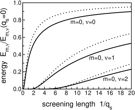
Figure 4: Bound-state energies $E_{m,\nu}$ as a function of inverse screening wavenumber $1/q_{s}$ for the first three $m=0$ states in Stern-Howard (solid lines) and Tanguy (dotted lines) potentials. All values are normalised by the corresponding energies for the unscreened potential, $E_{m,\nu}(q_{s}=0)=-(m+\nu+1/2)^{-2}$.

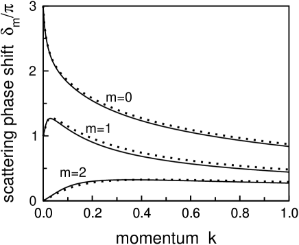
Figure 5: Scattering phase shifts $\delta_{m}$ as a function of the in-plane momentum $k$ for $1/q_{s}=5$. Solid lines: Stern-Howard potential; dotted lines: Tanguy potential.

1.10 Conclusions

We have shown that the accidental degeneracy in the energy eigenvalues of the 2D Kepler problem may be explained by the existence of a planar analogue of the familiar 3D Runge-Lenz vector. By moving into momentum space and making a stereographic projection onto a 3D sphere, a new integral relation in terms of special functions has been obtained, which to our knowledge has not previously been tabulated. This approach has also yielded the momentum-space eigenfunctions for bound states, which will prove useful in future applications. We have also demonstrated explicitly that the components of the 2D Runge-Lenz vector in real space are intimately related to infinitesimal rotations in 3D momentum space. Although no further insight has been gained into the screened exciton problem, this is more than compensated for by the unexpected beauty of the unscreened case.

With regard to the numerical expression (8) for critical screening lengths, it is still possible that it remains exactly true for both the Stern-Howard and Tanguy potentials. Tanguy’s results are inconclusive: the semi-classical approximation remains an approximation, and it is possible that rounding errors in the numerical evaluation of the integral (114) lead to its deviation from $\pi$. Indeed, it is interesting that the difference between the two potentials changes sign at $q_{s}\sim 1$, which allows for the fact that Eq. (8) may be simultaneously true for both potentials.

The obvious extension of the 2D hydrogenic problem is to consider scattering states as well as bound states, in order to obtain a complete set of basis functions. However, rather than projection onto a sphere, this would require the 2D momentum space to be projected onto a two-sheeted hyperboloid. This has been done for the 3D hydrogen atom [20], but the eigenfunctions are found to consist of two solutions, arising from the switching between sheets of the hyperboloid. Because of this complexity it is unlikely that the momentum-space eigenfunctions will produce any useful integral relations when compared with real-space solutions.

2 Anyon exciton: exact solutions

2.1 Motivation

Intrinsic photoluminescence experiments have revealed interesting features in the optical spectra of incompressible quantum liquids (IQLs) at filling factors $\nu=1/3$, $2/3$ and $2/5$ [44, 45, 46]. The anyon exciton model (AEM) was developed to provide a model of an exciton consisting of a valence hole and three quasielectrons (anyons) against the background of $\nu=1/3$ and $2/3$ IQLs [47], and has provided major insights into the role of electron-hole separation in determining their optical spectra. Recent developments in experimental techniques for studying such systems [48, 49] have rekindled our interest in developing a more general form of the model which may be applied to higher fractions. To this end, we seek a generalised form of the AEM for a neutral exciton made up of a valence hole and an arbitrary number $N$ of anyons. The particular case of $N=5$ allows us to consider an exciton against the background of an IQL with filling factor $\nu=2/5$.

2.2 Quantum Hall effects

The quantum Hall effect (QHE) was discovered in 1980 by von Klitzing et al. [50], who studied an effectively 2D electron system at high magnetic field and low temperature. The Hall conductivity $\sigma_{xy}$ exhibits plateaus at integer multiples of $e^{2}/h$ (corresponding to an integer number of filled Landau levels), and is accompanied by a vanishing diagonal conductivity $\sigma_{xx}$. This quantisation is independent of the shape of the specimen or presence of impurities and is accurate to one part in ten million, leading to its use as a standard of electrical resistance.

Another significant breakthrough was made in 1982 by Tsui et al. [51], who investigated higher-mobility semiconductor samples at increased magnetic fields and lower temperatures. Plateaus in $\sigma_{xy}$ were observed at fractional values of $e^{2}/h$, accompanied by minima in $\sigma_{xx}$. It soon became apparent that this phenomenon, labelled the fractional quantum Hall effect (FQHE), could not be explained in terms of a single-electron formulation; any theory would need to take into account the strongly-correlated behaviour of many electrons. (For a comprehensive review of the integer and fractional quantum Hall effects see [52, 53].)

In 1983, Laughlin showed [54] that the stability of the system at fractional filling factor (number of filled Landau levels) is due to the condensation of the electron system into an incompressible quantum liquid (IQL). By analogy with Jastrow wavefunctions in the theory of ⁴He, Laughlin proposed a many-electron variational wavefunction for filling factor $\nu=1/m$ ($m$ odd) to describe the ground state of the IQL:

$$\psi=\prod_{j<k}(z_{j}-z_{k})^{m}\prod_{l}\exp\left(-|z_{l}|^{2}/4\right),\vspace{3mm}$$ (118)

where $z_{i}$ are the complex electron coordinates scaled in units of magnetic length, and $m$ is an odd integer. He also noted the existence of an energy gap between the ground and excited states of the IQL, and predicted that excitations would be quasiparticles with fractional charge – quasielectrons and quasiholes. The first evidence for the existence of energy gaps was soon provided by magnetotransport experiments [55] and spectroscopic methods [56, 57], and magnetotransport measurements also provided a signature of charge fractionalisation [58, 59, 60].

An alternative to Laughlin’s method was provided by Haldane [61], who considered a system based on a spherical geometry in which the electrons are confined to the surface of a sphere with a magnetic monopole at the centre. Numerical diagonalisation of systems with up to eight electrons for $\nu=1/3$ in a spherical geometry [62] confirmed the accuracy of Laughlin’s wavefunction in describing the ground state, as well as the presence of a finite energy gap between ground and excited states. This work was later extended to $\nu=1/5$ with similar results [63]. The use of Haldane’s spherical geometry in numerical models of an exciton against the background of an IQL is considered in Section 2.4.

Further progress on the nature of the quasiparticle excitations was made by Halperin [64], who developed pseudo-wavefunctions to describe low-lying excited states in terms of a small number of quasiparticles added to the IQL ground state. These pseudo-wavefunctions are of the form

$$\Psi=P(z_{k})\prod_{j<k}\left(z_{j}-z_{k}\right)^{\alpha}\prod_{l=1}^{N}\exp\left\{-|z_{l}|^{2}/(4m)\right\},$$ (119)

where $z_{i}$ are the complex coordinates of the $N$ quasiparticles, $\alpha$ is a statistical factor and $P(z_{i})$ is a symmetric polynomial in the variables $z_{i}$. Halperin then used this method to construct the whole hierarchy of fractional states. From the quantisation rules that determine the allowed quasiparticle spacings he also determined that the quasiparticles are anyons obeying fractional statistics, i.e. the wavefunction changes by a complex phase factor when two particles are interchanged. (For more details on anyons and fractional statistics see [65, 66].)

In addition to charged quasiparticles, the IQL also supports dispersive neutral excitations. The lowest branch of these neutral excitations is labelled a magnetoroton [67, 68], and can be pictured as a quasielectron-quasihole pair. Strong evidence of the existence of these excitations has been provided by inelastic light scattering (Raman scattering) experiments [69].

Returning to Laughlin’s wavefunction, a picture began to emerge of magnetic ‘vortices’ generated by flux quanta, where the position of each vortex corresponds to a zero of the many-body wavefunction. The $\nu=1/3$ FQHE, for example, could be interpreted as the attachment of three flux quanta to each electron, forming composite bosons [70]. Stability of the system at this filling factor then corresponds to a Bose condensate of these composite particles.

The failure of this model to account for higher-order states with odd denominator, as well as even-denominator states, led to the development by Jain of the composite fermion model [71, 72]. Vortices are again attached to electrons, but the fractional quantum Hall effect becomes an integer quantum Hall effect for the new composite particles. For example, in the $\nu=1/3$ state each electron is considered bound to two flux quanta, such that the composite particle feels an effective field of one flux quantum per particle. These composites can then be considered as fermions filling one Landau level. The composite fermion model is generally accepted as providing the best current description of higher-order FQHE states (although not everyone subscribes to this view [73]), as well as a method for generating many-particle wavefunctions and their excitations.

One further development that should be mentioned is the recent direct observation of fractionally-charged quasiparticles in ‘shot noise’ measurements [74, 75]. This noise arises from a current of individual quasielectrons with charge $-e/3$ tunnelling through a narrow barrier (see [76] for more details). Whereas similar claims [77] have been questioned in the past, the results do look extremely promising, and a great deal of work is being carried out to verify these observations.

2.3 Photoluminescence experiments

Although the earliest experimental work on the FQHE was based on magnetotransport experiments, these only allowed energies near the Fermi level to be probed. The introduction of spectroscopic techniques was a significant step as it enabled the whole spectrum of energies to be studied via contactless measurements. The ideal system for such optical experiments is a GaAs-AlGaAs heterostructure. Donors are placed in the layer of higher-bandgap material (AlGaAs) and the electrons associated with these donors move towards the region of lower-bandgap material (GaAs). This process, known as modulation doping, creates a high-mobility two-dimensional electron gas (2DEG) in the layer of GaAs, which may be used as the basis for experimental study of the IQL. However, the electric field that is used to create the 2DEG also repels photoexcited holes, which necessitates adding a second barrier to restrict these holes. The physical system can be modelled by two parallel planes separated by a distance of $h$ magnetic lengths. It has been found that when $h=0$ the system possesses a hidden symmetry and is insensitive to electron correlations [78, 79] (This is analogous to the familiar Kohn theorem, which states that the excitation spectrum of a translationally-invariant system is unaffected by electron-electron interactions [80].) As a result, the frequencies of all allowed transitions coincide exactly with those of an empty crystal. For this reason, charge asymmetric systems (with $h\neq 0$) are the most interesting for experimental observation.

The phenomenon of photoluminescence also requires some explanation. Illumination of the semiconductor heterostructure produces non-equilibrium electrons and holes, which may then recombine radiatively via two different mechanisms. In extrinsic photoluminescence, electrons recombine with holes localised on acceptor dopants, introduced via $\delta$-doping, whereas in intrinsic photoluminescence electrons recombine with ‘free’ holes.

Experiments to study extrinsic emission provided the first optical measurement of FQHE energy gaps [56, 57], and a corresponding theory has been developed with good success [81]. Of most interest to the present work, however, are experiments on intrinsic PL. The first such experiments were by Heiman et al. [44, 45], who studied high-mobility GaAs-AlGaAs multiple quantum wells at varying filling factor. In this real system the hidden symmetry is broken, thus allowing electron correlation effects to influence the optical spectra. Several intrinsic emission lines were observed in the photoluminescence spectrum for $\nu<1$, and the most significant feature was a doublet near $\nu=2/3$ which had a similar temperature dependence to the magnetoresistance associated with the IQL in transport experiments. The authors later studied a higher-mobility single quantum well, which led to the observation of a similar doublet at filling factors $\nu=1/3$ and $2/5$. The results for $\nu=2/3$ were also reported by Turberfield et al. [46].

The only experimental work to study the effects of electron-hole separation on intrinsic photoluminescence was that by Plentz et al. [48]. Their apparatus allowed the 2DEG density to be changed by using applied gate voltages. This enabled the effective electron-hole separation (in units of magnetic length) to be varied, while keeping the filling factor constant (for more experimental details see [82]). The PL spectra obtained for $\nu=1/3$ show a pronounced doublet structure. With increasing electron-hole separation, the energy splitting of the doublet decreases and the higher-energy peak dominates. Refinements to this technique have recently been reported by another group [83, 84], and a similar method, which uses variations in the light intensity to change the 2DEG density, has also been developed [49, 85].

These experimental methods have a great deal of potential for further investigation of spatially-separated systems. Although little work has been done in this area, it is hoped that the present study and subsequent work will rekindle interest in this direction.

2.4 Theoretical studies

Any attempt to model intrinsic PL must take into account low-energy excitonic bound states (due to electron-hole Coulomb attraction) against the background of an IQL. The first such work was by Apalkov et al. [86, 87, 88, 89, 90], who numerically diagonalised systems comprising a small number of electrons together with a valence hole on the surface of a Haldane sphere. The electron-hole interaction was modified to take into account the layer separation $h$, which allowed both symmetric and asymmetric systems to be studied. Energy spectra were calculated for a range of values of $h$ and exciton branches were classified in terms of the exciton internal angular momentum $L$. For $h\leqslant 1.5l$, where $l$ is the magnetic length, there was a single exciton branch with $L=0$, whereas for $h>1.5l$ new branches appeared, with higher values of $L$ reaching down to become the ground state. The branches were labelled as either tight excitons or anyon excitons. For small $h$, the $L=0$ tight exciton forms the ground state, and as $h$ is increased, anyon exciton branches form a succession of ground states and the tight excitons move to higher energies.

Emission spectra were also calculated, and these also showed a strong dependence on $h$. For $h\lesssim 0.5l$ a single peak was observed, whereas for $h\gtrsim 0.5l$ a second lower-energy peak appears. A tentative interpretation of these results says that the upper peak is from direct transitions for exciton momentum $k=0$, whereas the lower peak corresponds to magnetoroton-assisted transitions with finite $k$. The double-peak structure shows a qualitative agreement with experiment [45, 82]. The results of Apalkov et al. were supported by a similar numerical study by Zang and Birman [91], who also produced PL spectra for different $h$ and obtained the familiar doublet structure.

In parallel with finite-size calculations, an analytical model of an exciton against the background of an IQL was formulated by Portnoi and Rashba [47, 92, 93, 94, 95], termed the anyon exciton model (AEM). This model is applicable for electron-hole separation $h\gtrsim 2l$, and thus complements the numerical approach. Indeed, remarkable agreement with finite-size results is obtained for $h\approx 2l$. Initially, the simplest model of a hole with two semions (quasielectrons with charge $-e/2$) was considered, but this was soon extended to a more-realistic four-particle exciton consisting of a hole and three quasielectrons with charge $-e/3$. The results of the AEM showed a multiple-branch energy spectrum, and a full set of exciton basis functions were obtained. More details of the formulation and results of the AEM can be found below.

2.5 Review of anyon exciton model

2.5.1 Formulation

We present here a brief overview of the anyon exciton model (AEM) applied to the case of a four-particle exciton [47]. The model considers a neutral exciton consisting of a valence hole with charge $+e$ and three quasielectrons (anyons) with charge $-e/3$ and statistical factor $\alpha$, subject to a strong perpendicular magnetic field $\mathbf{H}$. The hole and anyons move in two different planes separated by a distance of $h$ magnetic lengths. (Note that from now on we measure all distances in terms of the magnetic length $l=(c\hbar/eH)^{1/2}$ unless otherwise specified.)

This four-particle exciton will have a total of four degrees of freedom if all the particles are in the lowest Landau level. As the exciton is neutral we may assign it an in-plane momentum $\mathbf{k}$, which absorbs two of these degrees of freedom. The remaining degrees of freedom result in internal quantum numbers and a multiple-branch energy spectrum. Indeed, the two internal quantum numbers are assigned the labels $L$ and $M$, and enumerate exciton branches. Note that for $\mathbf{k}=0$, $L$ is related to the projection of the angular momentum $L_{z}$.

To simplify the description of the exciton, the hole and anyons are considered as moving in the same plane, and the separation $h$ can be introduced later as it does not appear in the exciton wavefunction. It is also convenient to move from the in-plane hole and anyon coordinates $\mathbf{r}_{h}$ and $\mathbf{r}_{i}$ to the new 2D coordinates

$$\mathbf{R}=\frac{1}{2}\left(\mathbf{r}_{h}+\frac{1}{3}\sum_{i=1}^{3}\>\mathbf{r}_{i}\right),\quad\boldsymbol{\rho}=\frac{1}{3}\sum_{i=1}^{3}\>\mathbf{r}_{i}-\mathbf{r}_{h},\quad\mathbf{r}_{jl}=\mathbf{r}_{j}-\mathbf{r}_{l},\vspace{3mm}$$ (120)

where $jl=12$, $23$ and $31$, together with the complex coordinates $z_{jl}=x_{jl}+iy_{jl}$. In Eq. (120), $\mathbf{R}$ is the coordinate of the geometrical centre of charge of the exciton, $\boldsymbol{\rho}$ is the position of the centre of negative charge relative to the hole, and $\mathbf{r}_{jl}$ are difference coordinates between pairs of anyons. The following constraint should also be noted:

$$\mathbf{r}_{12}+\mathbf{r}_{23}+\mathbf{r}_{31}=0,$$ (121)

which greatly simplifies the subsequent formulation.

The motion of an anyon exciton is described by a Halperin pseudo-wavefunction [64]:

$$\Psi(\mathbf{R},\boldsymbol{\rho},\{\bar{z}_{jl}\})=\frac{1}{\sqrt{2\pi A}}\exp\left\{i\mathbf{k}\cdot\mathbf{R}+\frac{i}{2}\hat{\mathbf{z}}\cdot[\boldsymbol{\rho}\times\mathbf{R}]-\frac{1}{4}(\boldsymbol{\rho}-\mathbf{d})^{2}\right\}\\ \times P_{L}(\ldots,\bar{z_{jl}},\ldots)\prod_{jl}(\bar{z}_{jl})^{\alpha}\exp\left\{-|z_{jl}|^{2}/36\right\},$$ (122)

where $A$ is the area of the sample and $P_{L}$ is a homogeneous polynomial of degree $L$ in the difference coordinates. Note that the statistical factor $\alpha=0$ for bosons, $\alpha=1$ for fermions, $\alpha=-1/3$ for quasielectrons in a $\nu=1/3$ IQL and $\alpha=+1/3$ for quasielectrons in a $\nu=2/3$ IQL.

The properties of the polynomial $P_{L}$ are of the utmost importance. By definition it is symmetric in the anyon coordinates $\bar{z}_{j}$, but the permutation rules with respect to the difference coordinates $\bar{z}_{jl}$ are not obvious. Indeed, it turns out that if $L$ is even, $P_{L}$ is symmetric in $\bar{z}_{jl}$, whereas if $L$ is odd, the polynomial is antisymmetric in $\bar{z}_{jl}$. For $L=3$, the simplest case, this polynomial is a Vandermonde determinant:

$$W\left(\bar{z}_{12},\bar{z}_{23},\bar{z}_{31}\right)=\left|\begin{array}[]{ccc}1&1&1\\ \bar{z}_{12}&\bar{z}_{23}&\bar{z}_{31}\\ {\bar{z}_{12}}^{2}&{\bar{z}_{23}}^{2}&{\bar{z}_{31}}^{2}\end{array}\right|=(\bar{z}_{12}-\bar{z}_{23})(\bar{z}_{23}-\bar{z}_{31})(\bar{z}_{31}-\bar{z}_{12}).$$ (123)

The linearly-independent $L$-even polynomials can be chosen as

$$P_{L,M}({\bar{z}_{12}},{\bar{z}_{23}},{\bar{z}_{31}})={\bar{z}_{12}}^{L-4M}{\bar{z}_{23}}^{2M}{\bar{z}_{31}}^{2M}+{\bar{z}_{23}}^{L-4M}{\bar{z}_{31}}^{2M}{\bar{z}_{12}}^{2M}+{\bar{z}_{31}}^{L-4M}{\bar{z}_{12}}^{2M}{\bar{z}_{23}}^{2M},$$ (124)

where the quantum number $M$ enumerates different polynomials with the same degree $L$. The total number of $L$-even polynomials with a given $L$ is therefore $[L/6]+1$, where the brackets $[\;]$ denote the integer part. The $L$-odd polynomials are constructed as follows:

$$P_{3,0}=W,\quad P_{L,M}=WP_{L-3,M},$$ (125)

and there are $[(L-3)/6]+1$ of these polynomials for a given $L$.

Given an expression for the exciton basis functions $\Psi_{i}$ in terms of the quantum numbers $\mathbf{k}$, $L$ and $M$, any exciton wavefunction may be expressed in terms of this basis:

$$\Phi=\sum_{i}\chi_{i}\Psi_{i}.\vspace{3mm}$$ (126)

However, the basis functions are not orthogonal in $M$, so the Schrödinger equation is written as follows:

$$\hat{H}\boldsymbol{\chi}=\varepsilon\hat{B}\boldsymbol{\chi},$$ (127)

where $\hat{B}$ is the overlap matrix of scalar products and $\varepsilon$ is an energy eigenvalue. The evaluation of the matrix elements $\hat{H}$ and $\hat{B}$ is rather complicated, and the reader is referred to [47] for further details. These matrix elements allow the calculation of the energy spectra and electron density for the exciton, and these results are outlined below.

2.5.2 Results

For energy eigenvalue calculations at $k=0$, a comparison of the energy for statistical factor $\alpha=-1/3$ and $\alpha=0$ shows good agreement for $h>2$ (see Fig. 1 in [47]), and hence a boson approximation is made to simplify further calculations. For $k\neq 0$, the energy spectra must be calculated numerically, and it is found that in the region $h>2$ the ground state of the system has non-zero angular momentum $L=3m$, where $m\geqslant 2$ is an integer. Note also that the wavefunctions of these ground states contain the polynomials $P_{6M,M}$ and $WP_{6M,M}$. These satisfy the hard-core constraint, in that they go to zero if any two of the anyon coordinates are the same. This is very encouraging as hard-core functions are the accepted standard for a proper description of anyons [96, 97].

Energy spectra for $h=2$ and $3$ are shown in Fig. 6 [47]. For $h=2$, the minimum of the spectrum occurs for non-zero $k$, which means that the exciton in the lowest energy state possesses a non-zero dipole moment. The negative dispersion in Fig. 6(a) arises because of the mutual repulsion of $L=2$ and $L=3$ branches. For higher values of $h$ the ground state is always at $k=0$, as in Fig. 6(b), and the lowest-branch dispersion is always positive.

Figure 6: Anyon exciton dispersion $\varepsilon(k)$ for two values of electron-hole separation $h$. Numbers show $L$ values; $h$ is in units of magnetic length $l$ and $\varepsilon$ is in units of the Coulomb energy $\varepsilon_{c}=e^{2}/\epsilon l$.

Calculations of the electron density around the hole also lead to remarkable results (see Fig. 7 [47]). For $k=0$ there is a crater-like dip in the density around the origin; this is an obvious signature of charge fractionalisation as a normal magnetoexciton always has a maximum at this point.

Figure 7: Electron density distribution in an anyon exciton for different values of the exciton in-plane momentum $k$. The distance $h$ between the hole and the incompressible electron liquid is equal to two magnetic lengths. The hole is at the origin; the $x$-axis is chosen along the exciton dipole moment.

The distribution for non-zero $k$ clearly shows two anyons close to the hole and a single anyon at a slight distance from it, providing further clear evidence of charge fractionalisation in anyon excitons.

2.6 Exciton basis functions

2.6.1 Derivation

The concept of exciton basis functions is now generalised [98] to an exciton consisting of a valence hole with charge $+e$ and $N$ anyons with charge $-e/N$ and statistical factor $\alpha$. The hole and anyons reside in two different layers, separated by a distance of $h$ magnetic lengths, and are subject to a magnetic field $\mathbf{H}=H\hat{\mathbf{z}}$ perpendicular to their planes of confinement. Unless otherwise stated, we shall assume that the hole and the quasielectrons are in their corresponding lowest Landau levels. To simplify the description of the exciton, the hole and anyons may be considered as moving in the same plane with coordinates $\mathbf{r}_{h}$ and $\mathbf{r}_{j}$, respectively, and the the layer separation $h$ can be introduced later when considering the anyon-hole interaction.

An exciton consisting of a hole and $N$ anyons, all in the lowest Landau level, will have a total of $N+1$ degrees of freedom. Assigning the exciton an in-plane momentum $\mathbf{k}$ absorbs two of these degrees of freedom, so for $N\geqslant 2$ the exciton will have $N-1$ internal degrees of freedom. At this stage we consider the particles as non-interacting and introduce interactions later as necessary. We can therefore write the $(N+1)$-particle Hamiltonian as

$$\hat{H}_{0}=\frac{1}{2m_{h}}\left({\hat{\mathbf{p}}}_{h}-\frac{q_{h}\mathbf{A}}{c}\right)^{2}+\sum_{j=1}^{N}\>\frac{1}{2m_{a}}\left({\hat{\mathbf{p}}}_{j}-\frac{q_{a}\mathbf{A}}{c}\right)^{2},\vspace{3mm}$$ (128)

where $q_{h}=+e$ and $q_{a}=-e/N$ are the hole and anyon charges, respectively.

Choosing the symmetric gauge

$$\mathbf{A}=\frac{1}{2}\left[\mathbf{H}\times\mathbf{r}\right],$$ (129)

and scaling all distances with the magnetic length $l=(c\hbar/eH)^{1/2}$, we obtain

$$\hat{H}_{0}=\frac{1}{2m_{h}}\left(\frac{1}{i}\nabla_{h}-\left[\hat{\mathbf{z}}\times\mathbf{r}_{h}\right]\right)^{2}+\sum_{j=1}^{N}\>\frac{1}{2m_{a}}\left(\frac{1}{i}\nabla_{j}+\frac{1}{N}\left[\hat{\mathbf{z}}\times\mathbf{r}_{j}\right]\right)^{2},\vspace{3mm}$$ (130)

where, as usual, $e$, $\hbar$ and $c$ are assumed equal to unity.

We now introduce the following new coordinates (see Fig. 8):

$$\mathbf{R}=\frac{1}{2}\left(\mathbf{r}_{h}+\frac{1}{N}\sum_{j=1}^{N}\>\mathbf{r}_{j}\right),\quad\boldsymbol{\rho}=\mathbf{r}_{h}-\frac{1}{N}\sum_{j=1}^{N}\>\mathbf{r}_{j},\quad\boldsymbol{\xi}_{j}=\mathbf{r}_{j}-\frac{1}{N}\sum_{l=1}^{N}\>\mathbf{r}_{l},\vspace{3mm}$$ (131)

together with the complex coordinates $\zeta_{j}=\xi_{xj}+i\xi_{yj}$. Note also the following constraint on these coordinates:

$$\sum_{j=1}^{N}\>\boldsymbol{\xi}_{j}=\sum_{j=1}^{N}\>\zeta_{j}=0.\vspace{3mm}$$ (132)

Figure 8: Two-dimensional coordinate system for hole and $N$ anyons ($C$ indicates the centre of negative charge). The hole is considered as being in the same plane as the anyons, with layer separation introduced as required.

The fact that the variables $\boldsymbol{\xi}_{j}$ are not independent means that derivatives with respect to these variables are not defined. However, it is possible to introduce the derivatives $\nabla_{\boldsymbol{\xi}_{j}}$ which treat the variables $\boldsymbol{\xi}_{j}$ as if they were independent [99].

Let $S$ be the $2N$-dimensional space of physical coordinates $\mathbf{r}_{j}$, and $S_{\xi}$ be the $2N$-dimensional space of the independent coordinates $\boldsymbol{\xi}_{j}$. Due to the constraint above, physical motion only takes place within a submanifold $M_{\xi}\subset S_{\xi}$, so $\xi$ maps the physical space $S$ to the submanifold $M_{\xi}$, i.e. $\xi:S\rightarrow M_{\xi}$. An arbitrary complex function $f$ can always be expressed explicitly as a function of the coordinates $\boldsymbol{\xi}_{j}$, and so we can write that $f$ maps $M_{\xi}$ to $\mathbb{C}$, i.e. $f:M_{\xi}\rightarrow\mathbb{C}$. If we now keep the expression for $f$ fixed, we can extend its definition over the whole space $S_{\xi}$ by removing the constraint, and it is now correct to talk about its derivatives $\nabla_{\boldsymbol{\xi}_{j}}f(\ldots,\boldsymbol{\xi}_{j},\ldots)$.

We may now consider a composition of the two maps $S\stackrel{{\scriptstyle\xi}}{{\rightarrow}}M_{\xi}\subset S_{\xi}\stackrel{{\scriptstyle f}}{{\rightarrow}}\mathbb{C}$ (see Fig. 9).

Figure 9: Wavefunction of relative motion expressed as a composition of two mappings $S\stackrel{{\scriptstyle\xi}}{{\rightarrow}}M_{\xi}\subset S_{\xi}\stackrel{{\scriptstyle f}}{{\rightarrow}}\mathbb{C}$.

Wavefunctions of the kind used to describe motion with respect to the centre of charge of the anyon subsystem are compositions of $f$ and $\xi$, such that

$$(f\circ\xi)(\mathbf{r}_{1},\ldots,\mathbf{r}_{N})=f(\ldots,\boldsymbol{\xi}_{j}(\mathbf{r}_{1},\ldots,\mathbf{r}_{N}),\ldots).$$ (133)

We do not distinguish between $f$ and $f\circ\xi$ in what follows, but rather write both as $f$.

Using the chain rule, we may now rewrite the derivatives of $f$ with respect to $\mathbf{r}_{j}$ as

$$\nabla_{j}f =\sum_{l=1}^{N}\>\nabla_{\boldsymbol{\xi}_{l}}f(\ldots,\boldsymbol{\xi}_{l},\ldots)\nabla_{j}\xi_{l}$$

$$=\nabla_{\boldsymbol{\xi}_{j}}f(\ldots,\boldsymbol{\xi}_{j},\ldots)-\frac{1}{N}\sum_{l=1}^{N}\>\nabla_{\boldsymbol{\xi}_{l}}f(\ldots,\boldsymbol{\xi}_{l},\ldots).\vspace{3mm}$$ (134)

We may now express the old coordinates in terms of the new ones as follows:

$$\mathbf{r}_{h}=\mathbf{R}+\frac{\boldsymbol{\rho}}{2},\quad\mathbf{r}_{j}=\mathbf{R}-\frac{\boldsymbol{\rho}}{2}+\boldsymbol{\xi}_{j},$$ (135)

and the derivatives with respect to the old coordinates are therefore

$$\nabla_{h} =\frac{1}{2}\nabla_{\mathbf{R}}+\nabla_{\boldsymbol{\rho}},$$ (136)

$$\nabla_{j} =\frac{1}{2N}\nabla_{\mathbf{R}}-\frac{1}{N}\nabla_{\boldsymbol{\rho}}+\nabla_{\boldsymbol{\xi}_{j}}-\frac{1}{N}\sum_{l=1}^{N}\>\nabla_{\boldsymbol{\xi}_{l}}.\vspace{3mm}$$ (137)

It is now possible to write the Hamiltonian (130) in terms of the new variables. Using Eqs. (2.6.1)–(137) we obtain

$$\hat{H}_{0}=\hat{H}_{exc}+\hat{H}_{\xi},$$ (138)

where

$$\hat{H}_{exc}=\frac{1}{2m_{h}}\left\{\frac{1}{2i}\nabla_{\mathbf{R}}+\frac{1}{i}\nabla_{\boldsymbol{\rho}}-\frac{1}{2}\left[\hat{\mathbf{z}}\times\left(\mathbf{R}-\frac{\boldsymbol{\rho}}{2}\right)\right]\right\}^{2}\\ +\frac{1}{2Nm_{a}}\left\{\frac{1}{2i}\nabla_{\mathbf{R}}-\frac{1}{i}\nabla_{\boldsymbol{\rho}}+\frac{1}{2}\left[\hat{\mathbf{z}}\times\left(\mathbf{R}+\frac{\boldsymbol{\rho}}{2}\right)\right]\right\}^{2},$$ (139)

and

$$\hat{H}_{\xi}=\frac{1}{2m_{a}}\sum_{j=1}^{N}\left\{\frac{1}{i}\nabla_{\boldsymbol{\xi}_{j}}-\frac{1}{Ni}\sum_{l=1}^{N}\nabla_{\boldsymbol{\xi}_{l}}+\frac{1}{2N}\left[\hat{\mathbf{z}}\times\boldsymbol{\xi}_{j}\right]\right\}^{2}.\vspace{3mm}$$ (140)

Note that Eq. (140) was obtained by applying constraint (132).

The first part $\hat{H}_{exc}$ is similar to that for a standard diamagnetic exciton [100, 101], with the electron mass replaced with $N$ anyon masses. The eigenfunctions of this operator can be written straightforwardly as

$$\Psi_{exc}(\mathbf{R},\boldsymbol{\rho})=\exp\left\{i\mathbf{k}\cdot\mathbf{R}+i\hat{\mathbf{z}}\cdot\left[\mathbf{R}\times\boldsymbol{\rho}\right]/2\right\}\Phi(\boldsymbol{\rho}),$$ (141)

where $\Phi(\boldsymbol{\rho})$ satisfies the equation

$$\left(\frac{1}{2m_{h}}\left\{\frac{1}{i}\nabla_{\boldsymbol{\rho}}-\frac{\left[\hat{\mathbf{z}}\times\left(\boldsymbol{\rho}-\mathbf{d}\right)\right]}{2}\right\}^{2}+\frac{1}{2Nm_{a}}\left\{\frac{1}{i}\nabla_{\boldsymbol{\rho}}+\frac{\left[\hat{\mathbf{z}}\times\left(\boldsymbol{\rho}-\mathbf{d}\right)\right]}{2}\right\}^{2}\right)\Phi=E_{exc}\Phi.\vspace{3mm}$$ (142)

Here, $\mathbf{d}=\mathbf{k}\times\hat{\mathbf{z}}$ is the exciton dipole moment. Note that Eq. (141) does not contain the mass-dependent phase factor that appears in the wavefunction in [101]. This is due to our choice of the centre of charge of the exciton for our coordinate $\mathbf{R}$, rather than the centre of mass chosen in [100, 101]. Thus, the quantum number $\mathbf{k}$ entering Eq. (141) represents the momentum of the geometrical centre of the exciton.

The solutions of Eq. (142) are

$$\Phi_{nm}=|\boldsymbol{\rho}|^{|m|}L_{n}^{|m|}\left\{(\boldsymbol{\rho}-\mathbf{d})^{2}/2\right\}\exp\left\{im\phi-(\boldsymbol{\rho}-\mathbf{d})^{2}/4\right\},$$ (143)

where $\phi$ is the azimuthal angle of the vector $(\boldsymbol{\rho}-\mathbf{d})$ and $L_{n}^{m}(z)$ are the associated Laguerre polynomials. The corresponding eigenvalues are

$$E_{exc}=\frac{1}{m_{h}}\left(n+\frac{|m|-m+1}{2}\right)+\frac{1}{Nm_{a}}\left(n+\frac{|m|+m+1}{2}\right).\vspace{3mm}$$ (144)

Note that in Eqs. (143) and (144) we no longer restricted ourselves to the lowest Landau level for the hole and quasielectrons. For the ground-state ($n,m=0$), Eq. (141) reduces to

$$\Psi_{exc}(\mathbf{R},\boldsymbol{\rho})=\exp\left\{i\mathbf{k}\cdot\mathbf{R}+i\hat{\mathbf{z}}\cdot\left[\mathbf{R}\times\boldsymbol{\rho}\right]/2-(\boldsymbol{\rho}-\mathbf{d})^{2}/4\right\},$$ (145)

which depends on the quantum number $\mathbf{k}$ alone.

We now move to consider the term $\hat{H}_{\xi}$ in Eq. (140), which may be divided into two parts:

$$\hat{H}_{1\xi}=\frac{1}{2m_{a}}\left(1-\frac{1}{N}\right)\sum_{j=1}^{N}\left(\frac{1}{i}\nabla_{\boldsymbol{\xi}_{j}}+\frac{1}{2N}\left[\hat{\mathbf{z}}\times{\boldsymbol{\xi}}_{j}\right]\right)^{2},\vspace{3mm}$$ (146)

and

$$\hat{H}_{2\xi}=\frac{1}{2Nm_{a}}\sum_{j=1}^{N}\Bigg{\{}-\nabla_{\boldsymbol{\xi}_{j}}^{2}+\frac{1}{Ni}\left[\hat{\mathbf{z}}\times{\boldsymbol{\xi}}_{j}\right]\cdot\left(\nabla_{\boldsymbol{\xi}_{j}}-\sum_{l=1}^{N}\nabla_{\boldsymbol{\xi}_{l}}\right)\\ +\frac{1}{N^{2}}|{\boldsymbol{\xi}_{j}}|^{2}+2\nabla_{\boldsymbol{\xi}_{j}}\cdot\left(\sum_{l=1}^{N}\nabla_{\boldsymbol{\xi}_{l}}\right)-\frac{1}{N}\left(\sum_{l=1}^{N}\nabla_{\boldsymbol{\xi}_{l}}\right)^{2}\Bigg{\}}.$$ (147)

The eigenfunctions of the ground state of $\hat{H}_{1\xi}$ can then be written in terms of complex coordinates as

$$\Phi_{\xi}=\prod_{j}\left(\bar{\zeta}_{j}\right)^{\beta_{j}}\exp\left\{-|\zeta_{j}|^{2}/4N\right\},\vspace{3mm}$$ (148)

with the corresponding eigenvalues

$$E_{\xi}=\frac{1}{2m_{a}}\left(1-\frac{1}{N}\right).\vspace{3mm}$$ (149)

If we now apply constraint (132), we find that the function $\Phi_{\xi}$ is also an eigenfunction of $\hat{H}_{2\xi}$, with a corresponding eigenvalue of zero, i.e.

$$\hat{H}_{2\xi}\Phi_{\xi}\propto\left(\sum_{j=1}^{N}{\boldsymbol{\xi}}_{j}\right)^{2}\Phi_{\xi}=0.\vspace{3mm}$$ (150)

A calculation of the total energy of the ground state gives

$$E=E_{exc}+E_{\xi}=\frac{1}{2m_{h}}+\frac{1}{2m_{a}}=\frac{1}{2}(\omega_{h}+N\omega_{a}),\vspace{3mm}$$ (151)

which is indeed the ground-state energy of the original $(N+1)$-particle Hamiltonian in Eq. (130).

The most general form for the ground-state eigenfunction of $\hat{H}_{0}$ is

$$\Psi\left(\mathbf{R},\boldsymbol{\rho},\{\bar{\zeta}_{i}\}\right)=\exp\left\{i\mathbf{k}\cdot\mathbf{R}+i\hat{\mathbf{z}}\cdot\left[\mathbf{R}\times\boldsymbol{\rho}\right]/2-(\boldsymbol{\rho}-\mathbf{d})^{2}/4\right\}\\ \times\quad F(\ldots,\bar{\zeta}_{i},\ldots)\prod_{p}\exp\left\{-|\zeta_{p}|^{2}/4N\right\},$$ (152)

where $F$ is a function of the complex conjugates $\bar{\zeta}_{i}$ alone. We choose $F$ as follows to satisfy the interchange rules for anyons:

$$F(\ldots,\bar{\zeta}_{i},\ldots)=P_{L}(\ldots,\bar{\zeta}_{i},\ldots)\prod_{j<l}(\bar{\zeta}_{j}-\bar{\zeta}_{l})^{\alpha},\vspace{3mm}$$ (153)

where $P_{L}$ is a symmetric polynomial of degree $L$ in the variables $\bar{\zeta}_{i}$. Note that for $\mathbf{k}=0$ the problem has rotational symmetry about the $z$-axis and the degree of the symmetric polynomial $L$ is related to the exciton angular momentum $[L_{z}=-L-N(N-1)\alpha/2]$.

We are now in a position to express the anyon exciton basis functions in the final form

$$\Psi\left(\mathbf{R},\boldsymbol{\rho},\{\zeta_{i}\}\right)=\exp\left\{i\mathbf{k}\cdot\mathbf{R}+i\hat{\mathbf{z}}\cdot\left[\mathbf{R}\times\boldsymbol{\rho}\right]/2-(\boldsymbol{\rho}-\mathbf{d})^{2}/4\right\}\\ \times\quad P_{L}(\ldots,\bar{\zeta}_{i},\ldots)\prod_{j<l}(\bar{\zeta}_{j}-\bar{\zeta}_{l})^{\alpha}\prod_{p}\exp\left\{-|\zeta_{p}|^{2}/4N\right\}.$$ (154)

2.6.2 Symmetric polynomials

We now consider the precise structure of the symmetric polynomials $P_{L}$ which appear in Eq. (154). To determine the symmetric basis polynomials of order $L$, we apply the fundamental theorem of symmetric polynomials [102], which states that any symmetric polynomial in $N$ variables, $P(x_{1},\ldots,x_{N})$, can be uniquely expressed in terms of the elementary symmetric polynomials

$$\sigma_{1}=\sum_{i}x_{i},\;\sigma_{2}=\sum_{i<j}x_{i}x_{j},\;\sigma_{3}=\sum_{i<j<k}x_{i}x_{j}x_{k},\;\ldots\;,\;\sigma_{N}=x_{1}x_{2}\cdots x_{N}.\vspace{3mm}$$ (155)

It is apparent that all linearly-independent symmetric basis polynomials of a particular degree may be enumerated by considering the possible products of the elementary symmetric polynomials (155), as the total degree $L$ is the sum of the degrees of the constituent polynomials. For example, the possible symmetric polynomials of degree four are constructed from $\sigma_{1}^{4}$, $\sigma_{1}^{2}\sigma_{2}$, $\sigma_{1}\sigma_{3}$, $\sigma_{2}^{2}$ and $\sigma_{4}$.

There are two further problems. The first is to determine the number of possible products of elementary symmetric polynomials for a total degree $L$. The second is to determine the structure of these products.

To calculate the number of linearly-independent symmetric basis polynomials of degree $L$ which may be constructed from the elementary symmetric polynomials $\sigma_{1},\ldots,\sigma_{N}$, we use a result from the theory of partitions [103].

The number of ways of partitioning a number $L$ into parts of size $1,2,\ldots,P$ is given by the coefficient of $x^{L}$ in the expansion of

$$\frac{1}{1-x}\cdot\frac{1}{1-x^{2}}\cdots\frac{1}{1-x^{P}}=\prod_{k=1}^{P}\;\frac{1}{1-x^{k}},\vspace{3mm}$$ (156)

where each term in the product is known as a generating function. The number of ways of partitioning increases rapidly with $L$ and does not follow any pattern. Furthermore, the different products of elementary symmetric polynomials for a particular value of $L$ must be determined by hand. An approximate formula for calculating the number of ways of partitioning a number does exist, the so-called Hardy-Ramanujan formula [104], but it is not applicable to the present case as we have no polynomial of order one due to constraint (132). This constraint significantly reduces the number of possible symmetric polynomials by removing the first factor in the product (156). For example, for $N=3$ the number of polynomials of degree $L$ is equal to the integer part of $L/6+1$ for even $L$ and the integer part of $(L-3)/6+1$ for odd $L$, which corresponds to the result obtained in [47].

2.6.3 Discussion

The key difference between the current general formulation and that outlined in [47] for the four-particle case $(N=3)$ is the replacement of anyon difference coordinates $\bar{z}_{jl}$ by the new coordinates $\bar{\zeta}_{i}$. The principal advantage of the difference coordinates was that they simplified the calculation of inter-anyon repulsion matrix elements, as well as the form of the statistical factor in the exciton wavefunction. However, they had the disadvantage that the classification of symmetric polynomials was more difficult, as it was necessary to introduce a Vandermonde determinant for odd-$L$ polynomials. For example, in the simplest case $L=3$, even though the number of anyon coordinates is the same in both formulations, we have $\sigma_{3}=(\bar{z}_{12}-\bar{z}_{23})(\bar{z}_{23}-\bar{z}_{31})(\bar{z}_{31}-\bar{z}_{12})$ in terms of difference coordinates, whereas we have a simple product $\sigma_{3}=\bar{\zeta}_{1}\bar{\zeta}_{2}\bar{\zeta}_{3}$ in terms of the new coordinates. For a number of anyons greater than three this disadvantage is crucial, as the classification of polynomials in terms of $\bar{z}_{jl}$ becomes too cumbersome and the number of constraints on these coordinates is greater than one.

2.7 Reformulation of four-particle anyon exciton

2.7.1 Formulation

We now use the above results to formulate the problem of a four-particle exciton in terms of the new coordinates $\bar{\zeta}_{i}$. We consider an exciton consisting of a hole and three anyons with charge $-e/3$, and make a boson approximation so that the statistical factor $\alpha=0$. As mentioned in Section 2.5.2, it is evident from Fig. 1 of [47] that for large values of $h$ (required for the AEM to be valid) the statistical factor $\alpha$ becomes unimportant, and the results for $\alpha=0$ were very similar to those for $\alpha=\pm 1/3$. We are therefore justified in approximating the anyons as bosons.

The basis functions for a four-particle anyon exciton in a boson approximation are, from Eq. (154):

$$\Psi\left(\mathbf{R},\boldsymbol{\rho},\bar{\zeta}_{1},\bar{\zeta}_{2},\bar{\zeta}_{3}\right)=\exp\left\{i\mathbf{k}\cdot\mathbf{R}+i\hat{\mathbf{z}}\cdot\left[\mathbf{R}\times\boldsymbol{\rho}\right]/2-(\boldsymbol{\rho}-\mathbf{d})^{2}/4\right\}\\ \times P_{L,M}(\bar{\zeta}_{1},\bar{\zeta}_{2},\bar{\zeta}_{3})\prod_{p=1}^{3}\exp\left\{-|\zeta_{p}|^{2}/12\right\},$$ (157)

where the index $M$ enumerates different linearly-independent symmetric polynomials of degree $L$.

As a result of constraint (132), $\sigma_{1}=\bar{\zeta}_{1}+\bar{\zeta}_{2}+\bar{\zeta}_{3}=0$, and so we need to consider only the elementary symmetric polynomials $\sigma_{2}$ and $\sigma_{3}$ when constructing the symmetric polynomial $P_{L,M}$ . From Eq. (156), the number of possible ways of constructing a polynomial of degree $L$ is the coefficient of $x^{L}$ in the expansion

$$\frac{1}{1-x^{2}}\cdot\frac{1}{1-x^{3}}=1+x^{2}+x^{3}+x^{4}+x^{5}+2x^{6}+x^{7}+2x^{8}+\ldots\;.\vspace{3mm}$$ (158)

Table 1 shows the possible ways of constructing the first twelve polynomials $P_{L}$.

Table 1: Possible ways of constructing a symmetric polynomial $P_{L}$ from the elementary symmetric polynomials $\sigma_{2}$ and $\sigma_{3}$.

Order, $L$	No. of polynomials	Structure
0	1	1
1	0	-
2	1	$\sigma_{2}$
3	1	$\sigma_{3}$
4	1	$\sigma_{2}^{2}$
5	1	$\sigma_{2}\sigma_{3}$
6	2	$\sigma_{2}^{3}$, $\sigma_{3}^{2}$
7	1	$\sigma_{2}^{2}\sigma_{3}$
8	2	$\sigma_{2}^{4}$, $\sigma_{2}\sigma_{3}^{2}$
9	2	$\sigma_{2}^{3}\sigma_{3}$, $\sigma_{3}^{3}$
10	2	$\sigma_{2}^{5}$, $\sigma_{2}^{2}\sigma_{3}^{2}$
11	2	$\sigma_{2}^{4}\sigma_{3}$, $\sigma_{2}\sigma_{3}^{3}$
12	3	$\sigma_{2}^{6}$, $\sigma_{2}^{3}\sigma_{3}^{2}$, $\sigma_{3}^{4}$

As in Section 2.5.1, a general exciton wavefunction for given $\mathbf{k}$ may be expanded in terms of the complete set of basis functions (157) as follows:

$$\Phi=\sum_{i}\chi_{i}\Psi_{i}.$$ (159)

Basis functions with different values of $\mathbf{k}$ are orthogonal. We shall later show that functions with different $L$ are also orthogonal. However, basis functions with the same value of $L$ but different $M$ are not necessarily orthogonal, so that their scalar products $\langle L,M|L,M^{\prime}\rangle$ will be non-zero. We therefore write the Schrödinger equation in matrix form as

$$\hat{H}\boldsymbol{\chi}=\varepsilon\hat{B}\boldsymbol{\chi},$$ (160)

where $\hat{B}$ is the block diagonal matrix of scalar products (the overlap matrix) and $\varepsilon$ is an energy eigenvalue. The size of each block in $\hat{B}$ depends on the number of different wavefunctions with given $L$. In the case of a four-particle exciton (see Table 1), the block corresponding to $L=12$ will be of size $3\times 3$. Both the overlap matrix $\hat{B}$ and the Hamiltonian matrix $\hat{H}$ are diagonal in $\mathbf{k}$. Note that for $\mathbf{k}=0$ the matrix $\hat{H}$ takes the same block diagonal form as $\hat{B}$ (as will be shown later), and as a result the problem becomes exactly solvable.

We shall now proceed to evaluate the matrix elements in Eq. (160). As $\hat{H}$ and $\hat{B}$ are diagonal in $\mathbf{k}$, in what follows we consider only the matrix elements diagonal in $\mathbf{k}$. Since all terms in the polynomial $P_{L,M}$ are of the form of a product of the coordinates ${\bar{\zeta}}_{j}$, we use the following functions in monomials in the matrix element calculations:

$$\Psi_{\{n\},\mathbf{k}}\left(\mathbf{R},\boldsymbol{\rho},\{\bar{\zeta_{i}}\}\right)=C\exp\left\{i\mathbf{k}\cdot\mathbf{R}+i\hat{\mathbf{z}}\cdot\left[\mathbf{R}\times\boldsymbol{\rho}\right]/2-(\boldsymbol{\rho}-\mathbf{d})^{2}/4\right\}\\ \times{\bar{\zeta}}_{1}^{n_{1}}{\bar{\zeta}}_{2}^{n_{2}}{\bar{\zeta}}_{3}^{n_{3}}\prod_{j=1}^{3}\exp\left\{-|\zeta_{j}|^{2}/12\right\},$$ (161)

where $\{n\}$ denotes the set of quantum numbers $n_{1}$, $n_{2}$ and $n_{3}$, and the constant $C$ will be defined in the next Section. The basis functions in terms of symmetric polynomials of degree $L$ can be obtained as a linear combination of the monomial functions (161), and $n_{1}+n_{2}+n_{3}=L$.

We also take into account constraint (132) via the following transformation:

$$\delta\left(\boldsymbol{\xi}_{1}+\boldsymbol{\xi}_{2}+\boldsymbol{\xi}_{3}\right)=\int\frac{d\mathbf{f}}{(2\pi)^{2}}\,\exp\left\{i\mathbf{f}\cdot\left(\boldsymbol{\xi}_{1}+\boldsymbol{\xi}_{2}+\boldsymbol{\xi}_{3}\right)\right\}.$$ (162)

2.7.2 Overlap matrix elements

To calculate the overlap matrix $\hat{B}$ we consider the scalar product of two monomial functions $\Psi_{\{n\},\mathbf{k}}$ and $\Psi_{\{n^{\prime}\},\mathbf{k}}$:

$$\langle\left\{n\right\}|\left\{n^{\prime}\right\}\rangle=\int d\mathbf{R}\int d\boldsymbol{\rho}\int\frac{d\mathbf{f}}{(2\pi)^{2}}\int d\boldsymbol{\xi}_{1}d\boldsymbol{\xi}_{2}d\boldsymbol{\xi}_{3}\\ \times\bar{\Psi}_{{\{n\},\mathbf{k}}}\Psi_{\{n^{\prime}\},\mathbf{k}}\exp\left\{i\mathbf{f}\cdot\left(\boldsymbol{\xi}_{1}+\boldsymbol{\xi}_{2}+\boldsymbol{\xi}_{3}\right)\right\}.$$ (163)

Integration over $\mathbf{R}$ and Gaussian integration over $\boldsymbol{\rho}$ give a factor of $2\pi A$, where $A$ is the area of the sample, and this yields

$$\langle\left\{n\right\}|\left\{n^{\prime}\right\}\rangle=C^{2}(2\pi A)\int\frac{d\mathbf{f}}{(2\pi)^{2}}\prod_{j=1}^{3}M_{n_{j}n_{j}^{\prime}}(\mathbf{f}),$$ (164)

where

$$M_{mm^{\prime}}(\mathbf{f})=\int d\boldsymbol{\xi}\>\zeta^{m}{\bar{\zeta}}^{m^{\prime}}e^{-\xi^{2}/6+i\mathbf{f}\cdot\boldsymbol{\xi}}.\vspace{3mm}$$ (165)

We now express the complex variable $\zeta$ in polar form as $\zeta=\xi e^{i\phi_{\boldsymbol{\xi}}}$, and let $\phi$ be the angle between $\mathbf{f}$ and $\boldsymbol{\xi}$, i.e.

$$\phi=\phi_{\boldsymbol{\xi}}-\phi_{\mathbf{f}}.$$ (166)

Eq. (165) then becomes

$$M_{mm^{\prime}}(\mathbf{f})=e^{i(m-m^{\prime})\phi_{\mathbf{f}}}\int_{0}^{2\pi}d\phi\int_{0}^{\infty}d\xi\>\zeta^{1+m+m^{\prime}}\\ \times\exp\left\{i(m-m^{\prime})\phi+if\xi\cos\phi-\xi^{2}/6\right\}.$$ (167)

The integration over $\phi$ can be carried out using Bessel’s integral [40]:

$$\int_{0}^{2\pi}d\phi\>e^{\pm i(m-m^{\prime})\phi+if\xi\cos\phi}=2\pi i^{|m-m^{\prime}|}J_{|m-m^{\prime}|}(f\xi),\vspace{3mm}$$ (168)

where $J_{m}(z)$ is a Bessel function of order $m$. This simplifies Eq. (167) to

$$M_{mm^{\prime}}(\mathbf{f})=2\pi i^{|m-m^{\prime}|}e^{i(m-m^{\prime})\phi_{\mathbf{f}}}\mathcal{M}_{mm^{\prime}}(f),$$ (169)

where we define

$$\mathcal{M}_{mm^{\prime}}(f)=\int_{0}^{\infty}d\xi\>\zeta^{1+m+m^{\prime}}e^{-\xi^{2}/6}J_{|m-m^{\prime}|}(f\xi).$$ (170)

The integral in Eq. (170) may be expressed [33] in terms of a confluent hypergeometric function $\Phi(\beta,\gamma;z)$ as

$$\mathcal{M}_{mm^{\prime}}(f)=\frac{2^{(m+m^{\prime})/2}3^{(m+m^{\prime})/2+1}\Gamma\left(\max\{m,m^{\prime}\}+1\right)}{|m-m^{\prime}|!}t^{|m-m^{\prime}|/2}\\ \times\Phi\left(\max\{m,m^{\prime}\}+1,|m-m^{\prime}|+1;-t\right),$$ (171)

where $t=3f^{2}/2$ and $\max\{m,m^{\prime}\}$ is the largest of the integers $m$ and $m^{\prime}$. Applying the Kummer transformation

$$\Phi(\beta,\gamma;-t)=e^{-t}\Phi(\gamma-\beta,\gamma;t),$$ (172)

simplifies Eq. (171) further. The fact that $(\gamma-\beta)$ is always a non-positive integer:

$$\gamma-\beta=|m-m^{\prime}|-\max\{m,m^{\prime}\},$$ (173)

means that $\Phi(\gamma-\beta,\gamma;t)$ reduces to a polynomial, and $\Phi(\beta,\gamma;-t)$ is then just a polynomial in $t$ multiplied by $e^{-t}$.

Integrating over $\phi_{\mathbf{f}}$ yields the final form of the overlap matrix elements

$$\langle\left\{n\right\}|\left\{n^{\prime}\right\}\rangle=C^{2}A(2\pi)^{3}\>\delta_{LL^{\prime}}\int_{0}^{\infty}df\>f\prod_{j=1}^{3}i^{|n_{j}-n^{\prime}_{j}|}\mathcal{M}_{n_{j}n^{\prime}_{j}}(f),\vspace{3mm}$$ (174)

where $L=n_{1}+n_{2}+n_{3}$. We define the constant $C$ so that for $L=L^{\prime}=0$ the matrix element $\langle\left\{n\right\}|\left\{n^{\prime}\right\}\rangle=\langle 0|0\rangle=1$, which gives

$$C^{2}=\frac{1}{3(2\pi)^{3}A}.$$ (175)

It should be noted that matrix elements in terms of symmetric polynomials can be constructed as a linear combination of the monomial matrix elements (174).

2.7.3 Anyon-anyon interaction

The interaction between anyons is of the form

$$\hat{V}_{aa}=\frac{1}{9}\left\{\frac{1}{\left|{\boldsymbol{\xi}}_{1}-{\boldsymbol{\xi}}_{2}\right|}+\frac{1}{\left|{\boldsymbol{\xi}}_{2}-{\boldsymbol{\xi}}_{3}\right|}+\frac{1}{\left|{\boldsymbol{\xi}}_{3}-{\boldsymbol{\xi}}_{1}\right|}\right\}.$$ (176)

Only matrix elements for the first term $\hat{V}_{12}$ will be calculated here as the others follow by analogy. Taking the Fourier transform of Eq. (176) yields

$$\hat{V}_{12}\left({\boldsymbol{\xi}}_{1},{\boldsymbol{\xi}}_{2}\right)=\frac{1}{9}\int\frac{d\mathbf{q}}{2\pi q}\exp\left\{i\mathbf{q}\cdot\left({\boldsymbol{\xi}}_{1}-{\boldsymbol{\xi}}_{2}\right)\right\},$$ (177)

which gives a matrix element

$$\langle\left\{n\right\}|\hat{V}_{12}|\left\{n^{\prime}\right\}\rangle=\frac{1}{9}\int d\mathbf{R}\int d\boldsymbol{\rho}\int\frac{d\mathbf{f}}{(2\pi)^{2}}\int\frac{d\mathbf{q}}{2\pi q}\int d\boldsymbol{\xi}_{1}d\boldsymbol{\xi}_{2}d\boldsymbol{\xi}_{3}\\ \times\bar{\Psi}_{{\{n\},\mathbf{k}}}\Psi_{\{n^{\prime}\},\mathbf{k}}\exp\left\{i\mathbf{f}\cdot\left(\boldsymbol{\xi}_{1}+\boldsymbol{\xi}_{2}+\boldsymbol{\xi}_{3}\right)\right\}\exp\left\{i\mathbf{q}\cdot\left({\boldsymbol{\xi}}_{1}-{\boldsymbol{\xi}}_{2}\right)\right\}.$$ (178)

Following the method of Section 2.7.2 gives

$$\langle\left\{n\right\}|\hat{V}_{12}|\left\{n^{\prime}\right\}\rangle =\frac{C^{2}(2\pi A)}{9}\prod_{j=1}^{3}i^{|n_{j}-n^{\prime}_{j}|}\int d\mathbf{f}\int d\mathbf{q}$$

$$\times\exp\left\{i\phi_{+}(n_{1}-n_{1}^{\prime})+i\phi_{-}(n_{2}-n_{2}^{\prime})+i\phi_{\mathbf{f}}(n_{3}-n_{3}^{\prime})\right\}$$

$$\times\mathcal{M}_{n_{1}n^{\prime}_{1}}(f_{+})\mathcal{M}_{n_{2}n^{\prime}_{2}}(f_{-})\mathcal{M}_{n_{3}n^{\prime}_{3}}(f),$$ (179)

where $\mathcal{M}_{mm^{\prime}}$ are as defined in Eq. (170), $\mathbf{f}_{\pm}=\mathbf{f}\pm\mathbf{q}$, and $\phi_{\pm}$ are the phases of $\mathbf{f}_{\pm}$.

We now eliminate $\phi_{\mathbf{f}}$ by the change of variables $\phi=\phi_{\mathbf{f}}-\phi_{\mathbf{q}}$ and $\psi_{\pm}=\phi_{\pm}-\phi_{\mathbf{f}}$. Substituting for $\phi_{\mathbf{f}}$, $\phi_{+}$ and $\phi_{-}$ in Eq. (2.7.3) and integrating over $\phi_{\mathbf{q}}$, we obtain

$$\langle\left\{n\right\}|\hat{V}_{12}|\left\{n^{\prime}\right\}\rangle =\frac{C^{2}A(2\pi)^{2}}{9}\>\delta_{LL^{\prime}}\prod_{j=1}^{3}i^{|n_{j}-n^{\prime}_{j}|}\int_{0}^{\infty}df\>f\int_{0}^{\infty}dq$$

$$\times\int_{0}^{2\pi}d\phi\>\exp\left\{i\phi(L-L^{\prime})\right\}\exp\left\{i\psi_{+}(n_{1}-n_{1}^{\prime})+i\psi_{-}(n_{2}-n_{2}^{\prime})\right\}$$

$$\times\mathcal{M}_{n_{1}n^{\prime}_{1}}(f_{+})\mathcal{M}_{n_{2}n^{\prime}_{2}}(f_{-})\mathcal{M}_{n_{3}n^{\prime}_{3}}(f),$$ (180)

where $\psi_{\pm}$ and $f_{\pm}$ can be expressed in terms of the variables of integration, $f$, $q$ and $\phi$, as

$$e^{i\psi_{\pm}}=\left(f\pm qe^{-i\phi}\right)/f_{\pm},\qquad f_{\pm}^{2}=f^{2}+q^{2}\pm 2fq\cos\phi.\vspace{3mm}$$ (181)

It is evident from Eq. (2.7.3) that the anyon-anyon interaction matrix has the same block diagonal structure as the overlap matrix. The integrand in Eq. (2.7.3) can be further reduced to a product of a polynomial in $q$, $f$ and $e^{\pm i\phi}$, and an exponential factor $\exp(-9f^{2}/2-3q^{2})$. This integral can therefore be evaluated analytically for any $\{n\}$ and $\{n^{\prime}\}$. For the case of $L=L^{\prime}=0$, using Eq. (175) for $C^{2}$, the anyon-anyon interaction matrix element reduces to

$$\langle 0|\hat{V}_{aa}|0\rangle=\frac{1}{6}\sqrt{\frac{\pi}{3}}.$$ (182)

2.7.4 Anyon-hole interaction

The anyon-hole interaction is of the form

$$\hat{V}_{ah}=-\frac{1}{3}\left\{\frac{1}{\left|\mathbf{r}_{1h}\right|}+\frac{1}{\left|\mathbf{r}_{2h}\right|}+\frac{1}{\left|\mathbf{r}_{3h}\right|}\right\},\vspace{3mm}$$ (183)

where we define

$$\mathbf{r}_{jh}=\boldsymbol{\xi}_{j}-\boldsymbol{\rho}+h\hat{\mathbf{z}}.\vspace{3mm}$$ (184)

Considering only $\hat{V}_{1h}$, we take the Fourier transform:

$$\hat{V}_{1h}\left(\boldsymbol{\rho},{\boldsymbol{\xi}}_{1}\right)=-\frac{1}{3}\int\frac{d\mathbf{q}}{(2\pi)^{2}}V_{ah}(q)\exp\left\{i\mathbf{q}\cdot\left({\boldsymbol{\xi}}_{1}-\boldsymbol{\rho}\right)\right\},\vspace{3mm}$$ (185)

where

$$V_{ah}(q)=\frac{2\pi}{q}e^{-qh}.\vspace{3mm}$$ (186)

The matrix elements are then

$$\langle\left\{n\right\}|\hat{V}_{1h}|\left\{n^{\prime}\right\}\rangle=-\frac{1}{3}\int d\mathbf{R}\int d\boldsymbol{\rho}\int\frac{d\mathbf{f}}{(2\pi)^{2}}\int\frac{d\mathbf{q}}{(2\pi)^{2}}V_{ah}(q)\int d\boldsymbol{\xi}_{1}d\boldsymbol{\xi}_{2}d\boldsymbol{\xi}_{3}\\ \times\bar{\Psi}_{{\{n\},\mathbf{k}}}\Psi_{\{n^{\prime}\},\mathbf{k}}\exp\left\{i\mathbf{f}\cdot\left(\boldsymbol{\xi}_{1}+\boldsymbol{\xi}_{2}+\boldsymbol{\xi}_{3}\right)\right\}\exp\left\{i\mathbf{q}\cdot\left({\boldsymbol{\xi}}_{1}-\boldsymbol{\rho}\right)\right\}.$$ (187)

Integration over $\mathbf{R}$ is straightforward and gives a factor of $A$. However, the integration over $\boldsymbol{\rho}$ is more complicated:

$$\int d\boldsymbol{\rho}\;\exp\left\{-(\boldsymbol{\rho}-\mathbf{d})^{2}/2-i\mathbf{q}\cdot\boldsymbol{\rho}\right\}=2\pi\exp(-q^{2}/2-i\mathbf{d}\cdot\mathbf{q}).\vspace{3mm}$$ (188)

Then, following the procedure in Section 2.7.2 once again, we obtain

$$\langle\left\{n\right\}|\hat{V}_{1h}|\left\{n^{\prime}\right\}\rangle =-\frac{C^{2}A}{3}\prod_{j=1}^{3}i^{|n_{j}-n^{\prime}_{j}|}\int d\mathbf{f}\int d\mathbf{q}\;V_{ah}(q)e^{-q^{2}/2-i\mathbf{d}\cdot\mathbf{q}}$$ (189)

$$\times\exp\left\{i\phi_{+}(n_{1}-n_{1}^{\prime})+i\phi_{\mathbf{f}}[(L-L^{\prime})-(n_{1}-n_{1}^{\prime})]\right\}$$

$$\times\mathcal{M}_{n_{1}n^{\prime}_{1}}(f_{+})\mathcal{M}_{n_{2}n^{\prime}_{2}}(f)\mathcal{M}_{n_{3}n^{\prime}_{3}}(f),$$

where $\mathcal{M}_{mm^{\prime}}$ are as defined in Eq. (170), $\mathbf{f}_{+}=\mathbf{f}+\mathbf{q}$, and $\phi_{+}$ is the phase of $\mathbf{f}_{+}$. As before, $L=n_{1}+n_{2}+n_{3}$.

We now eliminate $\phi_{\mathbf{f}}$ by substituting $\phi=\phi_{\mathbf{f}}-\phi_{\mathbf{q}}$ and $\psi=\phi_{+}-\phi_{\mathbf{f}}$. Choosing the $x$-axis along $\mathbf{d}$, the integration over $\phi_{\mathbf{q}}$ is then

$$\int_{0}^{2\pi}d\phi_{\mathbf{q}}\;\exp\left\{i\phi_{\mathbf{q}}(L-L^{\prime})-idq\cos\phi_{\mathbf{q}}\right\}=2\pi{(-i)}^{|L-L^{\prime}|}J_{|L-L^{\prime}|}(dq),\vspace{3mm}$$ (190)

which gives for the matrix elements:

$$\langle\left\{n\right\}|\hat{V}_{1h}|\left\{n^{\prime}\right\}\rangle =-\frac{C^{2}A(2\pi)^{2}}{3}i^{|L-L^{\prime}|}\prod_{j=1}^{3}i^{|n_{j}-n^{\prime}_{j}|}\int_{0}^{\infty}dq\;e^{-q^{2}/2-qh}J_{|L-L^{\prime}|}(dq)$$

$$\times\int_{0}^{\infty}df\>f\int_{0}^{2\pi}d\phi\>\exp\left\{i\phi(L-L^{\prime})+i\psi(n_{1}-n_{1}^{\prime})\right\}$$

$$\times\mathcal{M}_{n_{1}n^{\prime}_{1}}(f_{+})\mathcal{M}_{n_{2}n^{\prime}_{2}}(f)\mathcal{M}_{n_{3}n^{\prime}_{3}}(f),$$ (191)

where the new variables $\psi$ and $f_{+}$ can be expressed in terms of the variables of integration as

$$e^{i\psi}=\left(f+qe^{-i\phi}\right)/f_{+},\qquad f_{+}^{2}=f^{2}+q^{2}+2fq\cos\phi.$$ (192)

For $d=0$, the Bessel function $J_{|L-L^{\prime}|}(dq)$ entering the integrand of Eq. (2.7.4) is non-zero only if $L=L^{\prime}$. This indicates that for the case of zero in-plane momentum $(k=d=0)$, the anyon-hole interaction matrix has the same block diagonal structure as the anyon-anyon and overlap matrices. Therefore, states with different angular momentum $L_{z}$ decouple.

Eq. (2.7.4) may be simplified further using the explicit form of $\mathcal{M}_{mm^{\prime}}(f)$ in Eq. (171) and subsequent results. This yields the following expression for the anyon-hole interaction matrix elements for basis functions in terms of symmetric polynomials:

$$\langle L,M|\hat{V}_{ah}|L^{\prime},M^{\prime}\rangle=-\int_{0}^{\infty}\exp(-3q^{2}/2-qh)J_{|L-L^{\prime}|}(dq)Q_{LM,L^{\prime}M^{\prime}}(q)\;dq,$$ (193)

where $Q_{LM,L^{\prime}M^{\prime}}(q)$ is a polynomial in $q$ (the lowest order polynomial is $Q_{00,00}=1$). This expression was previously derived in [47]. Note that for zero 2DEG-hole separation $(h=0)$, Eq. (193) further reduces to an expression in terms of elementary functions. For the case of $k=d=0$ and $L=L^{\prime}=0$, the anyon-hole interaction matrix element is then

$$\langle 0|\hat{V}_{ah}|0\rangle=-\sqrt{\frac{\pi}{6}}.$$ (194)

2.8 Six-particle anyon exciton

2.8.1 Formulation

We now introduce an anyon exciton consisting of a hole and five anyons with charge $-e/5$. We also make a boson approximation so that the statistical factor $\alpha=0$. Our justification for this step is as follows. It was shown in [47] that for large values of $h$ (which is required for the AEM to be valid) the statistical factor $\alpha$ becomes unimportant, and the results for $\alpha=0$ were very similar to those for $\alpha=\pm 1/3$. We would therefore also expect this to be true for $\alpha=\pm 1/N$, as this is even closer to zero. From now on we consider a boson approximation $(\alpha=0)$ for anyon statistics.

The explicit form of the exciton basis functions is

$$\Psi_{L,M,\mathbf{k}}\left(\mathbf{R},\boldsymbol{\rho},\{\bar{\zeta_{i}}\}\right)=\exp\left\{i\mathbf{k}\cdot\mathbf{R}+i\hat{\mathbf{z}}\cdot\left[\mathbf{R}\times\boldsymbol{\rho}\right]/2-(\boldsymbol{\rho}-\mathbf{d})^{2}/4\right\}\\ \times P_{L,M}({\bar{\zeta}}_{1},\ldots,{\bar{\zeta}}_{5})\prod_{j=1}^{5}\exp\left\{-|\zeta_{j}|^{2}/20\right\},$$ (195)

where $M$ enumerates all linearly-independent symmetric polynomials of degree $L$.

To construct the symmetric polynomials $P_{L,M}$ we need to consider only the elementary symmetric polynomials $\sigma_{2}$, $\sigma_{3}$, $\sigma_{4}$ and $\sigma_{5}$. Note that $\sigma_{1}=0$ because of constraint (132). From Eq. (156), we find that the number of possible ways of constructing a polynomial of degree $L$ is therefore the coefficient of $x^{L}$ in the expansion

$$\frac{1}{1-x^{2}}\cdot\frac{1}{1-x^{3}}\cdot\frac{1}{1-x^{4}}\cdot\frac{1}{1-x^{5}}=1+x^{2}+x^{3}+2x^{4}+2x^{5}\\ +3x^{6}+3x^{7}+5x^{8}+5x^{9}+7x^{10}+\ldots\;.\vspace{3mm}$$ (196)

The possible ways of constructing the first twelve polynomials are shown explicitly in Table 2. It is evident that the number and complexity of the polynomials increases rapidly with the degree $L$.

Table 2: Possible ways of constructing a symmetric polynomial $P_{L}$ from the elementary symmetric polynomials $\sigma_{2}$, $\sigma_{3}$, $\sigma_{4}$ and $\sigma_{5}$.

Order, $L$	No. of polynomials	Structure
0	1	1
1	0	-
2	1	$\sigma_{2}$
3	1	$\sigma_{3}$
4	2	$\sigma_{2}^{2}$, $\sigma_{4}$
5	2	$\sigma_{2}\sigma_{3}$, $\sigma_{5}$
6	3	$\sigma_{2}^{3}$, $\sigma_{2}\sigma_{4}$, $\sigma_{3}^{2}$
7	3	$\sigma_{2}^{2}\sigma_{3}$, $\sigma_{2}\sigma_{5}$, $\sigma_{3}\sigma_{4}$
8	5	$\sigma_{2}^{4}$, $\sigma_{2}^{2}\sigma_{4}$, $\sigma_{2}\sigma_{3}^{2}$, $\sigma_{3}\sigma_{5}$, $\sigma_{4}^{2}$
9	5	$\sigma_{2}^{3}\sigma_{3}$, $\sigma_{2}^{2}\sigma_{5}$, $\sigma_{2}\sigma_{3}\sigma_{4}$, $\sigma_{3}^{3}$, $\sigma_{4}\sigma_{5}$
10	7	$\sigma_{2}^{5}$, $\sigma_{2}^{3}\sigma_{4}$, $\sigma_{2}^{2}\sigma_{3}^{2}$, $\sigma_{2}\sigma_{3}\sigma_{5}$, $\sigma_{2}\sigma_{4}^{2}$, $\sigma_{3}^{2}\sigma_{4}$, $\sigma_{5}^{2}$
11	7	$\sigma_{2}^{4}\sigma_{3}$, $\sigma_{2}^{3}\sigma_{5}$, $\sigma_{2}^{2}\sigma_{3}\sigma_{4}$, $\sigma_{2}\sigma_{3}^{3}$, $\sigma_{2}\sigma_{4}\sigma_{5}$,
		$\sigma_{3}^{2}\sigma_{5}$, $\sigma_{3}\sigma_{4}^{2}$
12	10	$\sigma_{2}^{6}$, $\sigma_{2}^{4}\sigma_{4}$, $\sigma_{2}^{3}\sigma_{3}^{2}$, $\sigma_{2}^{2}\sigma_{3}\sigma_{5}$, $\sigma_{2}^{2}\sigma_{4}^{2}$, $\sigma_{2}\sigma_{3}^{2}\sigma_{4}$,
		$\sigma_{2}\sigma_{5}^{2}$, $\sigma_{3}^{4}$, $\sigma_{3}\sigma_{4}\sigma_{5}$, $\sigma_{4}^{3}$

Following the method in Section 2.5.1 once again, we expand a general exciton wavefunction for given $\mathbf{k}$ in terms of the complete set of basis functions (195):

$$\Phi=\sum_{i}\chi_{i}\Psi_{i}.$$ (197)

As mentioned in Section 2.7.1, basis functions with different values of $\mathbf{k}$ and $L$ are orthogonal, although basis functions with the same value of $L$ but different $M$ are not necessarily orthogonal, so we introduce the overlap matrix $\hat{B}$ of scalar products into the Schrödinger equation as follows:

$$\hat{H}\boldsymbol{\chi}=\varepsilon\hat{B}\boldsymbol{\chi}.$$ (198)

Note that $\hat{B}$ is block diagonal, and in the case of a six-particle exciton (see Table 2), the block corresponding to $L=12$ for example will be of size $10\times 10$. As the Hamiltonian matrix $\hat{H}$ and the overlap matrix $\hat{B}$ are diagonal in $\mathbf{k}$, we only need to consider the matrix elements in Eq. (198) that are diagonal in $\mathbf{k}$. We use the following functions in monomials in the matrix element calculations, from which the basis functions in terms of symmetric polynomials can be obtained as a linear combination:

$$\Psi_{\{n\},\mathbf{k}}\left(\mathbf{R},\boldsymbol{\rho},\{\bar{\zeta_{i}}\}\right)=C\exp\left\{i\mathbf{k}\cdot\mathbf{R}+i\hat{\mathbf{z}}\cdot\left[\mathbf{R}\times\boldsymbol{\rho}\right]/2-(\boldsymbol{\rho}-\mathbf{d})^{2}/4\right\}\\ \times{\bar{\zeta}}_{1}^{n_{1}}{\bar{\zeta}}_{2}^{n_{2}}{\bar{\zeta}}_{3}^{n_{3}}{\bar{\zeta}}_{4}^{n_{4}}{\bar{\zeta}}_{5}^{n_{5}}\prod_{j=1}^{5}\exp\left\{-|\zeta_{j}|^{2}/20\right\},$$ (199)

where $\{n\}$ denotes the set of quantum numbers $n_{1}$ to $n_{5}$, for which it should be noted that $n_{1}+n_{2}+n_{3}+n_{4}+n_{5}=L$, and the constant $C$ will be defined in Section 2.8.2.

Constraint (132) is taken into account via the following transformation:

$$\delta\left(\boldsymbol{\xi}_{1}+\boldsymbol{\xi}_{2}+\boldsymbol{\xi}_{3}+\boldsymbol{\xi}_{4}+\boldsymbol{\xi}_{5}\right)=\int\frac{d\mathbf{f}}{(2\pi)^{2}}\,\exp\left\{i\mathbf{f}\cdot\left(\boldsymbol{\xi}_{1}+\boldsymbol{\xi}_{2}+\boldsymbol{\xi}_{3}+\boldsymbol{\xi}_{4}+\boldsymbol{\xi}_{5}\right)\right\}.\vspace{3mm}$$ (200)

2.8.2 Overlap matrix elements

To calculate the overlap matrix $\hat{B}$, let us consider the scalar product of two monomial functions:

$$\langle\left\{n\right\}|\left\{n^{\prime}\right\}\rangle=\int d\mathbf{R}\int d\boldsymbol{\rho}\int\frac{d\mathbf{f}}{(2\pi)^{2}}\int d\boldsymbol{\xi}_{1}d\boldsymbol{\xi}_{2}d\boldsymbol{\xi}_{3}d\boldsymbol{\xi}_{4}d\boldsymbol{\xi}_{5}\\ \times\bar{\Psi}_{{\{n\},\mathbf{k}}}\Psi_{\{n^{\prime}\},\mathbf{k}}\exp\left\{i\mathbf{f}\cdot\left(\boldsymbol{\xi}_{1}+\boldsymbol{\xi}_{2}+\boldsymbol{\xi}_{3}+\boldsymbol{\xi}_{4}+\boldsymbol{\xi}_{5}\right)\right\}.$$ (201)

The integration over $\mathbf{R}$ and $\boldsymbol{\rho}$ gives a factor of $2\pi A$, and this leaves the following:

$$\langle\left\{n\right\}|\left\{n^{\prime}\right\}\rangle=C^{2}(2\pi A)\int\frac{d\mathbf{f}}{(2\pi)^{2}}\;\prod_{j=1}^{5}M_{n_{j}n^{\prime}_{j}},\vspace{3mm}$$ (202)

where

$$M_{mm^{\prime}}(\mathbf{f})=\int d\boldsymbol{\xi}\>\zeta^{m}{\bar{\zeta}}^{m^{\prime}}e^{-\xi^{2}/10+i\mathbf{f}\cdot\boldsymbol{\xi}}.\vspace{3mm}$$ (203)

If we now make the substitution $\zeta=\xi e^{i\phi_{\boldsymbol{\xi}}}$, and let $\phi$ be the angle between $\mathbf{f}$ and $\boldsymbol{\xi}$, i.e.

$$\phi=\phi_{\boldsymbol{\xi}}-\phi_{\mathbf{f}},$$ (204)

where $\phi_{\mathbf{f}}$ is the phase of $\mathbf{f}$, we obtain

$$M_{mm^{\prime}}(\mathbf{f})=\exp\left\{i(m-m^{\prime})\phi_{\mathbf{f}}\right\}\int_{0}^{2\pi}d\phi\int_{0}^{\infty}d\xi\>\xi^{1+m+m^{\prime}}\\ \times\exp\left\{i(m-m^{\prime})\phi+if\xi\cos\phi-\xi^{2}/10\right\}.$$ (205)

We can now make use of Bessel’s integral

$$\int_{0}^{2\pi}d\phi\>e^{\pm i(m-m^{\prime})\phi+if\xi\cos\phi}=2\pi i^{|m-m^{\prime}|}J_{|m-m^{\prime}|}(f\xi),\vspace{3mm}$$ (206)

to reduce our expression to the form

$$M_{mm^{\prime}}(\mathbf{f})=2\pi i^{|m-m^{\prime}|}e^{i(m-m^{\prime})\phi_{\mathbf{f}}}\mathcal{M}_{mm^{\prime}}(f),$$ (207)

where

$$\mathcal{M}_{mm^{\prime}}(f)=\int_{0}^{\infty}d\xi\>\xi^{1+m+m^{\prime}}e^{-\xi^{2}/10}J_{|m-m^{\prime}|}(f\xi).\vspace{3mm}$$ (208)

This can also be expressed in terms of a confluent hypergeometric function $\Phi(\beta,\gamma;z)$ as

$$\mathcal{M}_{mm^{\prime}}(f)=\frac{2^{(m+m^{\prime})/2}5^{(m+m^{\prime})/2+1}\Gamma\left(\max\{m,m^{\prime}\}+1\right)}{|m-m^{\prime}|!}t^{|m-m^{\prime}|/2}\\ \times\Phi\left(\max\{m,m^{\prime}\}+1,|m-m^{\prime}|+1;-t\right),$$ (209)

where $t=5f^{2}/2$ and $\max\{m,m^{\prime}\}$ is the largest of the integers $m$ and $m^{\prime}$. Eq. (209) can be simplified further if we apply the Kummer transformation:

$$\Phi(\beta,\gamma;-t)=e^{-t}\Phi(\gamma-\beta,\gamma;t),$$ (210)

and note that $(\gamma-\beta)$ is always a negative integer:

$$\gamma-\beta=|m-m^{\prime}|-\max\{m,m^{\prime}\}.$$ (211)

This means that $\Phi(\gamma-\beta,\gamma;t)$ reduces to a polynomial, and $\Phi(\beta,\gamma;-t)$ is then just a polynomial multiplied by $e^{-t}$.

If we now perform the integration over $\phi_{\mathbf{f}}$ we obtain the final form of the overlap matrix elements

$$\langle\left\{n\right\}|\left\{n^{\prime}\right\}\rangle=C^{2}A(2\pi)^{5}\>\delta_{LL^{\prime}}\int_{0}^{\infty}df\>f\prod_{j=1}^{5}i^{|n_{j}-n^{\prime}_{j}|}\mathcal{M}_{n_{j}n^{\prime}_{j}}(f),$$ (212)

where $L=n_{1}+n_{2}+n_{3}+n_{4}+n_{5}$. Note that nothing depends on $\mathbf{k}$ in this expression for the matrix elements. It is convenient to define the constant $C$ so that for $L=L^{\prime}=0$ the matrix element $\langle\left\{n\right\}|\left\{n^{\prime}\right\}\rangle=\langle 0|0\rangle=1$. This yields

$$C^{2}=\frac{1}{125(2\pi)^{5}A}.$$ (213)

In the above formulation we have only considered matrix elements in terms of monomial functions. As mentioned earlier, matrix elements in terms of symmetric polynomials can be easily constructed as a linear combination of the monomial matrix elements (212).

2.8.3 Anyon-anyon interaction

The anyon-anyon interaction has the form

$$\hat{V}_{aa}=\frac{1}{25}\sum_{j<l}\;\frac{1}{|\boldsymbol{\xi}_{j}-\boldsymbol{\xi}_{l}|}.$$ (214)

We shall only calculate the matrix elements for the first term $\hat{V}_{12}$ as the others follow by analogy. We begin by taking the Fourier transform of Eq. (214):

$$\hat{V}_{12}\left({\boldsymbol{\xi}}_{1},{\boldsymbol{\xi}}_{2}\right)=\frac{1}{25}\int\frac{d\mathbf{q}}{2\pi q}\exp\left\{i\mathbf{q}\cdot\left({\boldsymbol{\xi}}_{1}-{\boldsymbol{\xi}}_{2}\right)\right\}.\vspace{3mm}$$ (215)

This gives a matrix element in terms of monomials

$$\langle\left\{n\right\}|\hat{V}_{12}|\left\{n^{\prime}\right\}\rangle =\frac{1}{25}\int d\mathbf{R}\int d\boldsymbol{\rho}\int\frac{d\mathbf{f}}{(2\pi)^{2}}\int\frac{d\mathbf{q}}{2\pi q}$$

$$\times\int d\boldsymbol{\xi}_{1}d\boldsymbol{\xi}_{2}d\boldsymbol{\xi}_{3}d\boldsymbol{\xi}_{4}d\boldsymbol{\xi}_{5}\>\bar{\Psi}_{{\{n\},\mathbf{k}}}\Psi_{\{n^{\prime}\},\mathbf{k}}$$

$$\times\exp\left\{i\mathbf{f}\cdot\left(\boldsymbol{\xi}_{1}+\boldsymbol{\xi}_{2}+\boldsymbol{\xi}_{3}+\boldsymbol{\xi}_{4}+\boldsymbol{\xi}_{5}\right)\right\}\exp\left\{i\mathbf{q}\cdot\left({\boldsymbol{\xi}}_{1}-{\boldsymbol{\xi}}_{2}\right)\right\}.$$ (216)

Following the procedure in Section 2.8.2 yields

$$\langle\left\{n\right\}|\hat{V}_{12}|\left\{n^{\prime}\right\}\rangle =\frac{C^{2}A(2\pi)^{3}}{25}\prod_{j=1}^{5}i^{|n_{j}-n^{\prime}_{j}|}\int d\mathbf{f}\int d\mathbf{q}$$

$$\times\exp\left\{i\phi_{+}(n_{1}-n_{1}^{\prime})+i\phi_{-}(n_{2}-n_{2}^{\prime})\right\}$$

$$\times\exp\left\{i\phi_{\mathbf{f}}\right[(n_{3}-n_{3}^{\prime})+(n_{4}-n_{4}^{\prime})+(n_{5}-n_{5}^{\prime})\left]\right\}$$

$$\times\mathcal{M}_{n_{1}n^{\prime}_{1}}(f_{+})\mathcal{M}_{n_{2}n^{\prime}_{2}}(f_{-})\prod_{j=3}^{5}\mathcal{M}_{n_{j}n^{\prime}_{j}}(f),\vspace{3mm}$$ (217)

where $\mathcal{M}_{mm^{\prime}}$ are as defined in Eq. (208), $\mathbf{f}_{\pm}=\mathbf{f}\pm\mathbf{q}$, and $\phi_{\pm}$ are the phases of $\mathbf{f}_{\pm}$.

We now seek to eliminate $\phi_{\mathbf{f}}$ by the change of variables $\phi=\phi_{\mathbf{f}}-\phi_{\mathbf{q}}$ and $\psi_{\pm}=\phi_{\pm}-\phi_{\mathbf{f}}$. After substitution and integration over $\phi_{\mathbf{q}}$ we obtain

$$\langle\left\{n\right\}|\hat{V}_{12}|\left\{n^{\prime}\right\}\rangle =\frac{C^{2}(2\pi)^{4}A}{25}\>\delta_{LL^{\prime}}\prod_{j=1}^{5}i^{|n_{j}-n^{\prime}_{j}|}\int_{0}^{\infty}df\>f\int_{0}^{\infty}dq\int_{0}^{2\pi}d\phi$$

$$\times\exp\left\{i\phi(L-L^{\prime})\right\}\exp\left\{i\psi_{+}(n_{1}-n_{1}^{\prime})+i\psi_{-}(n_{2}-n_{2}^{\prime})\right\}$$

$$\times\mathcal{M}_{n_{1}n^{\prime}_{1}}(f_{+})\mathcal{M}_{n_{2}n^{\prime}_{2}}(f_{-})\mathcal{M}_{n_{3}n^{\prime}_{3}}(f)\mathcal{M}_{n_{4}n^{\prime}_{4}}(f)\mathcal{M}_{n_{5}n^{\prime}_{5}}(f),\vspace{3mm}$$ (218)

where $\psi_{\pm}$ and $f_{\pm}$ can be expressed in terms of the variables of integration as

$$e^{i\psi_{\pm}}=\left(f\pm qe^{-i\phi}\right)/f_{\pm},\qquad f_{\pm}^{2}=f^{2}+q^{2}\pm 2fq\cos\phi.$$ (219)

Eq. (2.8.3) shows that the anyon-anyon interaction matrix has the same block diagonal structure as the overlap matrix. For the case of $L=L^{\prime}=0$, using Eq. (213) for $C^{2}$, the anyon-anyon interaction matrix element reduces to

$$\langle 0|\hat{V}_{aa}|0\rangle=\frac{1}{5}\sqrt{\frac{\pi}{5}}.$$ (220)

2.8.4 Anyon-hole interaction

The anyon hole interaction takes the form

$$\hat{V}_{ah}=-\frac{1}{5}\left\{\frac{1}{\left|\mathbf{r}_{1h}\right|}+\frac{1}{\left|\mathbf{r}_{2h}\right|}+\frac{1}{\left|\mathbf{r}_{3h}\right|}+\frac{1}{\left|\mathbf{r}_{4h}\right|}+\frac{1}{\left|\mathbf{r}_{5h}\right|}\right\},$$ (221)

where

$$\mathbf{r}_{jh}=\boldsymbol{\xi}_{j}-\boldsymbol{\rho}+h\hat{\mathbf{z}}.\vspace{3mm}$$ (222)

Considering only $\hat{V}_{1h}$, we take the Fourier transform:

$$\hat{V}_{1h}\left(\boldsymbol{\rho},{\boldsymbol{\xi}}_{1}\right)=-\frac{1}{5}\int\frac{d\mathbf{q}}{(2\pi)^{2}}V_{ah}(q)\exp\left\{i\mathbf{q}\cdot\left({\boldsymbol{\xi}}_{1}-\boldsymbol{\rho}\right)\right\},\vspace{3mm}$$ (223)

where

$$V_{ah}(q)=\frac{2\pi}{q}e^{-qh}.\vspace{3mm}$$ (224)

The matrix elements are then

$$\langle\left\{n\right\}|\hat{V}_{1h}|\left\{n^{\prime}\right\}\rangle =-\frac{1}{5}\int d\mathbf{R}\int d\boldsymbol{\rho}\int\frac{d\mathbf{f}}{(2\pi)^{2}}\int\frac{d\mathbf{q}}{(2\pi)^{2}}V_{ah}(q)$$

$$\times\int d\boldsymbol{\xi}_{1}d\boldsymbol{\xi}_{2}d\boldsymbol{\xi}_{3}d\boldsymbol{\xi}_{4}d\boldsymbol{\xi}_{5}\>\bar{\Psi}_{{\{n\},\mathbf{k}}}\Psi_{\{n^{\prime}\},\mathbf{k}}$$

$$\times\exp\left\{i\mathbf{f}\cdot\left(\boldsymbol{\xi}_{1}+\boldsymbol{\xi}_{2}+\boldsymbol{\xi}_{3}+\boldsymbol{\xi}_{4}+\boldsymbol{\xi}_{5}\right)\right\}\exp\left\{i\mathbf{q}\cdot\left({\boldsymbol{\xi}}_{1}-\boldsymbol{\rho}\right)\right\}.$$ (225)

Integration over $\mathbf{R}$ and $\boldsymbol{\rho}$ gives $2\pi A\exp\left(-q^{2}/2-i\mathbf{d}\cdot\mathbf{q}\right)$. Then, following the procedure in Section 2.8.2 once again, we obtain

$$\langle\left\{n\right\}|\hat{V}_{1h}|\left\{n^{\prime}\right\}\rangle =-\frac{C^{2}(2\pi)^{2}A}{5}\prod_{j=1}^{5}i^{|n_{j}-n^{\prime}_{j}|}\int d\mathbf{f}\int d\mathbf{q}\;V_{ah}(q)e^{-q^{2}/2-i\mathbf{d}\cdot\mathbf{q}}$$

$$\times\exp\left\{i\phi_{+}(n_{1}-n_{1}^{\prime})+i\phi_{\mathbf{f}}\left[(L-L^{\prime})-(n_{1}-n_{1}^{\prime})\right]\right\}$$

$$\times\mathcal{M}_{n_{1}n^{\prime}_{1}}(f_{+})\prod_{j=2}^{5}\mathcal{M}_{n_{j}n^{\prime}_{j}}(f),$$ (226)

where $\mathcal{M}_{mm^{\prime}}$ are as defined in Eq. (208), $\mathbf{f}_{+}=\mathbf{f}+\mathbf{q}$, and $\phi_{+}$ is the phase of $\mathbf{f}_{+}$. As before, $L=n_{1}+n_{2}+n_{3}+n_{4}+n_{5}$.

We now eliminate $\phi_{\mathbf{f}}$ by substituting $\phi=\phi_{\mathbf{f}}-\phi_{\mathbf{q}}$ and $\psi=\phi_{+}-\phi_{\mathbf{f}}$. Choosing $\mathbf{d}$ along the $x$-axis, the integration over $\phi_{\mathbf{q}}$ is then

$$\int_{0}^{2\pi}d\phi_{\mathbf{q}}\;\exp\left\{i\phi_{\mathbf{q}}(L-L^{\prime})-idq\cos\phi_{\mathbf{q}}\right\}=2\pi{(-i)}^{|L-L^{\prime}|}J_{|L-L^{\prime}|}(dq),\vspace{3mm}$$ (227)

which gives for the matrix elements:

$$\langle\left\{n\right\}|\hat{V}_{1h}|\left\{n^{\prime}\right\}\rangle =-\frac{C^{2}(2\pi)^{4}A}{5}{(-i)}^{|L-L^{\prime}|}\prod_{j=1}^{5}i^{|n_{j}-n^{\prime}_{j}|}$$

$$\times\int_{0}^{\infty}df\>f\int_{0}^{\infty}dq\>e^{-q^{2}/2-qh}J_{|L-L^{\prime}|}(dq)$$

$$\times\int_{0}^{2\pi}d\phi\;\exp\left\{i\phi(L-L^{\prime})+i\psi(n_{1}-n_{1}^{\prime})\right\}$$

$$\times\mathcal{M}_{n_{1}n^{\prime}_{1}}(f_{+})\prod_{j=2}^{5}\mathcal{M}_{n_{j}n^{\prime}_{j}}(f),$$ (228)

where $\psi$ and $f_{+}$ can be expressed in terms of the variables of integration as

$$e^{i\psi}=\left(f+qe^{-i\phi}\right)/f_{+},\qquad f_{+}^{2}=f^{2}+q^{2}+2fq\cos\phi.\vspace{3mm}$$ (229)

Eq. (2.8.4) may be simplified further, and this yields the following expression for the anyon-hole interaction matrix elements for basis functions in terms of symmetric polynomials:

$$\langle L,M|\hat{V}_{ah}|L^{\prime},M^{\prime}\rangle=-\int_{0}^{\infty}\exp(-5q^{2}/2-qh)J_{|L-L^{\prime}|}(dq)Q_{LM,L^{\prime}M^{\prime}}(q)\;dq,\vspace{3mm}$$ (230)

where $Q_{LM,L^{\prime}M^{\prime}}(q)$ is a polynomial in $q$ (the lowest order polynomial is $Q_{00,00}=1$). For $h=0$, Eq. (230) further reduces to an expression in terms of elementary functions. For the case of $L=L^{\prime}=0$, the anyon-hole interaction matrix element is then

$$\langle 0|\hat{V}_{ah}|0\rangle=-\sqrt{\frac{\pi}{10}}.$$ (231)

2.9 Exact results for $\mathbf{k}=0$, $L=0$

All the above results are simplified significantly for the state with $\mathbf{k}=0$ and $L=0$. For such a state, the $(N+1)$-particle wavefunction (154) with $\alpha=0$ reduces to the form

$$\Psi\left(\mathbf{R},\boldsymbol{\rho},\{\zeta_{i}\}\right)=C_{N}\exp\left\{i\hat{\mathbf{z}}\cdot\left[\mathbf{R}\times\boldsymbol{\rho}\right]/2-\rho^{2}/4\right\}\exp\left\{-\sum_{p=1}^{N}|\zeta_{p}|^{2}/4N\right\},\vspace{3mm}$$ (232)

where the normalisation constant $C_{N}$ can be determined from the integral

$$C_{N}^{2}\int d\mathbf{R}\int\frac{d\mathbf{f}}{{(2\pi)}^{2}}\int d\boldsymbol{\rho}\;e^{-\rho^{2}/2}\int d\boldsymbol{\xi}_{1}\cdots d\boldsymbol{\xi}_{N}\\ \times\exp\left\{\sum_{p=1}^{N}\left(i\boldsymbol{\xi}_{p}\cdot\mathbf{f}-\xi_{p}^{2}/2N\right)\right\}=\frac{C_{N}^{2}A}{N^{2}}(2\pi N)^{N}=1.$$ (233)

For the case of $\mathbf{k}=0$ and $L=0$, the interaction matrix elements of a $(N+1)$-particle exciton are straightforward to evaluate. The anyon-anyon matrix element is

$$\langle 0|\hat{V}_{aa}|0\rangle =\frac{N(N-1)}{2A(2\pi N)^{N}}\int d\mathbf{R}\int\frac{d\mathbf{q}}{2\pi q}\int d\boldsymbol{\rho}\;e^{-\rho^{2}/2}\int d\boldsymbol{\xi}_{1}\cdots d\boldsymbol{\xi}_{N}$$

$$\times\int\frac{d\mathbf{f}}{(2\pi)^{2}}\;\exp\left\{\sum_{p=1}^{N}\left(i\boldsymbol{\xi}_{p}\cdot\mathbf{f}-\xi_{p}^{2}/2N\right)+i\mathbf{q}\cdot\left(\boldsymbol{\xi}_{1}-\boldsymbol{\xi}_{2}\right)\right\}$$

$$=\frac{(N-1)}{4N}\sqrt{\frac{\pi}{N}}.\vspace{3mm}$$ (234)

For non-zero inter-plane separation $h$, the anyon-hole matrix element can be reduced to

$$\langle 0|\hat{V}_{ah}|0\rangle =-\frac{N^{2}}{A(2\pi N)^{N}}\int d\mathbf{R}\int\frac{d\mathbf{q}}{2\pi q}\int d\boldsymbol{\rho}\;e^{-\rho^{2}/2}\int d\boldsymbol{\xi}_{1}\cdots d\boldsymbol{\xi}_{N}$$

$$\times\int\frac{d\mathbf{f}}{(2\pi)^{2}}\exp\left\{\sum_{p=1}^{N}\left(i\boldsymbol{\xi}_{p}\cdot\mathbf{f}-\xi_{p}^{2}/2N\right)+i\mathbf{q}\cdot\left(\boldsymbol{\xi}_{1}-\boldsymbol{\rho}\right)-qh\right\}$$

$$=-\int_{0}^{\infty}dq\;e^{-Nq^{2}/2-qh}=-\sqrt{\frac{\pi}{2N}}e^{h^{2}/2N}\mbox{erfc}\left(h/\sqrt{2N}\right),\vspace{3mm}$$ (235)

where $\mbox{erfc}(x)$ is the complementary error function. (Note that for $h=0$, Eq. (2.9) can be simplified further to a numerical value.) Using the asymptotic expansion of $\mbox{erfc}(x)$ it can be easily seen from Eq. (2.9) that $\langle 0|\hat{V}_{ah}|0\rangle\rightarrow-1/h$ as $h\rightarrow\infty$, as expected.

Eqs. (2.9) and (2.9) also allow us to calculate the critical inter-plane separation $h_{c}$ at which the $\mathbf{k}=0$, $L=0$ state becomes unbound, i.e. when

$$\sqrt{\frac{\pi}{2N}}\;e^{x_{c}^{2}}\;\mbox{erfc}(x_{c})=\frac{(N-1)\sqrt{2}}{4N}\sqrt{\frac{\pi}{N}},\vspace{3mm}$$ (236)

where $x_{c}=h_{c}/\sqrt{2N}$. So, for $N=3$ the critical separation $h_{c}\approx 5.39\>l$, for $N=5$ we find that $h_{c}\approx 5.59\>l$, and for $N\gg 1$ we have $h_{c}\approx 1.32\sqrt{2N}\>l$. Notably, these critical separations are well inside the region for which the AEM is applicable. It should be emphasised that the state with $L=0$ is not the ground state for the anyon exciton at large separation $h$. For example, for a four-particle exciton [47], the ground states for large separation satisfy a superselection rule $L=3m$, where $m$ is an integer, and when $h\rightarrow\infty$ the ground state energy tends to its classical value, $\varepsilon_{cl}=-(2/3)^{3/2}/h$.

The model is applicable to real physical situations at large layer separations ($h>l$), although it remains solvable for all values of $h$, including $h=0$. Moreover, it has been shown in [47] that the ground state of the four-particle problem ($N=3$) at $h=0$ is the state with $\mathbf{k}=0$ and $L=0$. We expect the same to be true for $N\geqslant 5$, since the anyon-hole attraction will always overcome the anyon-anyon repulsion at small inter-particle separations. It can be shown (in a similar way to that in [47]) that the smallest average inter-particle separation corresponds to the $L=0$ case. Therefore, the case of $\mathbf{k}=0$, $L=0$ is of special interest since it predicts the anyon exciton binding energies in the limit $h\rightarrow 0$.

We are now in a position to write down a general expression for the binding energy of a $(N+1)$-particle exciton at zero 2DEG-hole separation ($h=0$):

$$E_{b}=-\left(\langle 0|\hat{V}_{ah}|0\rangle+\langle 0|\hat{V}_{aa}|0\rangle\right)=\left[1-\frac{(N-1)}{2\sqrt{2}N}\right]\sqrt{\frac{\pi}{2N}}.\vspace{3mm}$$ (237)

Eq. (237) has been written in this particular form to emphasise the key result that for any value of $N$ there always exists at least one bound state of a neutral $(N+1)$-particle anyon exciton. For $N=1$, Eq. (237) yields the value $\sqrt{\pi/2}$, which corresponds to that obtained in [101] for a standard diamagnetic exciton. For a four-particle exciton $(N=3)$, $E_{b}=\left(1-\sqrt{2}/6\right)\sqrt{\pi/6}$, which agrees with the result of [47]. Finally, for $N=5$ we have a binding energy of $(1-\sqrt{2}/5)\sqrt{\pi/10}$, which can also be obtained from Eqs. (220) and (231).

2.10 Conclusions

The anyon exciton model has been generalised to the case of a neutral exciton consisting of a valence hole and an arbitrary number $N$ of anyons, and several important mathematical results have been obtained. A complete set of exciton basis functions has been obtained and these functions have been fully classified using a result from the theory of partitions. We have derived expressions for the overlap and interaction matrix elements of a six-particle system $(N=5)$, which describes an exciton against the background of an IQL with filling factor $\nu=2/5$. In the particular case of $\mathbf{k}=0$ and $L=0$, we have found an expression for the binding energy of a $(N+1)$-particle exciton at zero anyon-hole separation, which agrees with known results for a standard diamagnetic exciton and four-particle anyon exciton. We have also shown that the $(N+1)$-particle exciton remains bound for 2DEG-hole separations exceeding several magnetic lengths, when the anyon exciton model becomes applicable to real physical systems.

3 Appendices

3.1 Solution of real-space Schrödinger equation in two dimensions

We apply the method of separation of variables to Eq. (39), making the substitution

$$\Psi(\boldsymbol{\rho})=R(\rho)\Phi(\phi).$$ (238)

Introducing a separation constant $m^{2}$, we can obtain the angular equation

$$\frac{d^{2}\Phi}{d\phi^{2}}+m^{2}\Phi=0,$$ (239)

with the solution

$$\Phi(\phi)=\frac{1}{\sqrt{2\pi}}e^{im\phi}.\vspace{3mm}$$ (240)

The corresponding radial equation (with $E=-q_{0}^{2}$) is

$$\frac{d^{2}R}{d\rho^{2}}+\frac{1}{\rho}\frac{dR}{d\rho}+\left(\frac{2}{\rho}-q_{0}^{2}-\frac{m^{2}}{\rho^{2}}\right)R=0.\vspace{3mm}$$ (241)

We make the substitution

$$R(\rho)=C\rho^{|m|}e^{-q_{0}\rho}w(\rho),$$ (242)

where $C$ is a normalisation constant. This leads to the equation

$$\rho\frac{d^{2}w}{d\rho^{2}}+(2|m|+1-2q_{0}\rho)\frac{dw}{d\rho}+(2-2|m|q_{0}-q_{0})w=0.$$ (243)

Making a final change of variables $\beta=2q_{0}\rho$, we obtain

$$\beta\frac{d^{2}w}{d\beta^{2}}+(2|m|+1-\beta)\frac{dw}{d\beta}+\left(\frac{1}{q_{0}}-|m|-\frac{1}{2}\right)w=0.\vspace{3mm}$$ (244)

This is the confluent hypergeometric equation [33], which has two linearly independent solutions. If we choose the solution which is regular at the origin, then this becomes a polynomial of finite degree if $q_{0}=(n+1/2)^{-1}$, with $n=0,1,2,\ldots$ Eq. (244) then becomes the associated Laguerre equation [40], the solutions of which are the associated Laguerre polynomials

$$w=L_{n-|m|}^{2|m|}(\beta)=L_{n-|m|}^{2|m|}(2q_{0}\rho).$$ (245)

We can now write the real-space wavefunction in the form

$$\Psi_{nm}(\boldsymbol{\rho})=\frac{C}{2\pi}\rho^{|m|}e^{-q_{0}\rho}L_{n-|m|}^{2|m|}(2q_{0}\rho)e^{im\phi_{\rho}},$$ (246)

where the reason for the subscript on $\phi$ is explained in Section 1.7.3.

To normalise this wavefunction we need to make use of the integral [40]:

$$\int_{0}^{\infty}e^{-2q_{0}\rho}(2q_{0}\rho)^{2|m|+1}L_{n-|m|}^{2|m|}(2q_{0}\rho)L_{n-|m|}^{2|m|}(2q_{0}\rho)\,d(2q_{0}\rho)\\ =\frac{(n+|m|)!}{(n-|m|)!}(2n+1).$$ (247)

The normalised wavefunctions are therefore:

$$\Psi_{nm}(\boldsymbol{\rho})=\sqrt{\frac{q_{0}^{3}(n-|m|)!)}{\pi(n+|m|)!}}(2q_{0}\rho)^{|m|}e^{-q_{0}\rho}L_{n-|m|}^{2|m|}(2q_{0}\rho)e^{im\phi_{\rho}},\vspace{3mm}$$ (248)

satisfying the following orthogonality condition:

$$\int\Psi_{n_{1}m_{1}}^{*}(\boldsymbol{\rho})\Psi_{n_{2}m_{2}}(\boldsymbol{\rho})\,d\boldsymbol{\rho}=\delta_{n_{1}n_{2}}\delta_{m_{1}m_{2}}.$$ (249)

3.2 Derivation of expression for $\hat{\mathbf{A}}^{2}$

From Eq. (41) we have

$$\hat{\mathbf{A}}^{2} =\left[(\hat{\mathbf{q}}\times\hat{\mathbf{L}}_{z}-\hat{\mathbf{L}}_{z}\times\hat{\mathbf{q}})-\frac{2}{\rho}\boldsymbol{\rho}\right]^{2}$$ (250)

$$=[2(\hat{\mathbf{q}}\times\hat{\mathbf{L}}_{z})-i\hat{\mathbf{q}}]^{2}-\frac{2}{\rho}\boldsymbol{\rho}\cdot[2(\hat{\mathbf{q}}\times\hat{\mathbf{L}}_{z})-i\hat{\mathbf{q}}]-\frac{2}{\rho}[2(\hat{\mathbf{q}}\times\hat{\mathbf{L}}_{z})-i\hat{\mathbf{q}}]\cdot\boldsymbol{\rho}+4.$$

We further expand as follows:

$$[2(\hat{\mathbf{q}}\times\hat{\mathbf{L}}_{z})-i\hat{\mathbf{q}}]^{2} =4(\hat{\mathbf{q}}\times\hat{\mathbf{L}}_{z})^{2}-2i\hat{\mathbf{q}}\cdot(\hat{\mathbf{q}}\times\hat{\mathbf{L}}_{z})-2i(\hat{\mathbf{q}}\times\hat{\mathbf{L}}_{z})\cdot\hat{\mathbf{q}}-\hat{\mathbf{q}}^{2}$$ (251)

$$=4\hat{\mathbf{q}}^{2}\hat{\mathbf{L}}_{z}^{2}+2\hat{\mathbf{q}}^{2}-\hat{\mathbf{q}}^{2}=\hat{\mathbf{q}}^{2}(4\hat{\mathbf{L}}_{z}^{2}+1),$$

and

$$-\frac{2}{\rho}\boldsymbol{\rho}\cdot[2(\hat{\mathbf{q}}\times\hat{\mathbf{L}}_{z})-i\hat{\mathbf{q}}]-\frac{2}{\rho}[2(\hat{\mathbf{q}}\times\hat{\mathbf{L}}_{z})-i\hat{\mathbf{q}}]\cdot\boldsymbol{\rho}=-\frac{2}{\rho}(4\hat{\mathbf{L}}_{z}^{2}+1).\vspace{3mm}$$ (252)

Substituting Eqs. (251) and (252) into Eq. (250) gives

$$\hat{\mathbf{A}}^{2}=\hat{\mathbf{q}}^{2}(4\hat{\mathbf{L}}_{z}^{2}+1)-\frac{2}{\rho}(4\hat{\mathbf{L}}_{z}^{2}+1)+4,$$ (253)

which, from Eq. (110), is just

$$\hat{\mathbf{A}}^{2}=\hat{H}(4\hat{\mathbf{L}}_{z}^{2}+1)+4.$$ (254)

3.3 Variable phase method

In this Section, which is based on the formulation in [3], we derive the basic equations of the variable phase approach in two dimensions from the radial Schrödinger equation. This derivation is similar to that in three dimensions [105].

3.3.1 Scattering phase shifts

The relative in-plane motion of two interacting particles with masses $M_{a}$ and $M_{b}$ and energy of relative motion $E$ can be considered as the motion of a particle with mass $\mu_{ab}=M_{a}M_{b}/(M_{a}+M_{b})$ and energy $E$, moving in an external central potential $V(\rho)$. This motion is described by a wavefunction satisfying the stationary Schrödinger equation

$$\hat{H}_{rel}\psi=-\frac{\hbar^{2}}{2\mu_{ab}}\left(\frac{1}{\rho}\frac{\partial}{\partial\rho}\rho\frac{\partial}{\partial\rho}+\frac{1}{\rho^{2}}\frac{\partial^{2}}{\partial\varphi^{2}}\right)\psi+V(\rho)\psi=E\psi.\vspace{3mm}$$ (255)

Owing to the axial symmetry of the potential $V(\rho)$, we can separate variables in the expression for the wavefunction

$$\psi_{m}(\rho,\varphi)=R_{m}(\rho)e^{im\varphi},\qquad m=0,\pm 1,\pm 2,\ldots\;.$$ (256)

The equation for the radial function $R_{m}(\rho)$ reads

$$R^{\prime\prime}_{m}+\frac{1}{\rho}R^{\prime}_{m}+\left(k^{2}-U(\rho)-\frac{m^{2}}{\rho^{2}}\right)R_{m}=0,$$ (257)

where $k^{2}=2\mu_{ab}E/\hbar^{2}$ and $U(\rho)=2\mu_{ab}V(\rho)/\hbar^{2}$. In what follows we consider $m\geq 0$ only, as $R_{-m}(\rho)=R_{m}(\rho)$.

We assume that the interaction potential vanishes at infinity (the precise decay rate will be discussed later). Then, at large distances the radial function satisfies the free Bessel equation, whose general solution is

$$R_{m}(\rho) =A_{m}[J_{m}(k\rho)\cos{\delta_{m}}-N_{m}(k\rho)\sin{\delta_{m}}]$$ (258)

$$\stackrel{{\scriptstyle\rho\rightarrow\infty}}{{\longrightarrow}}A_{m}\left(\frac{2}{\pi k\rho}\right)^{1/2}\cos(k\rho-(2m+1)\pi/4+\delta_{m}),$$

where $\delta_{m}$ is the scattering phase shift [1, 8], and $J_{m}(k\rho)$ and $N_{m}(k\rho)$ are the Bessel and Neumann functions, respectively.

In the variable phase approach, $A_{m}$ and $\delta_{m}$ are considered not as constants, but as functions of the distance $\rho$. The amplitude function $A_{m}(\rho)$ and the phase function $\delta_{m}(\rho)$ are introduced by the equation

$$R_{m}(\rho)=A_{m}(\rho)[J_{m}(k\rho)\cos{\delta_{m}(\rho)}-N_{m}(k\rho)\sin{\delta_{m}(\rho)}],$$ (259)

with an additional condition, which we are free to choose as

$$R^{\prime}_{m}(\rho)=A_{m}(\rho)[J^{\prime}_{m}(k\rho)\cos{\delta_{m}(\rho)}-N^{\prime}_{m}(k\rho)\sin{\delta_{m}(\rho)}],$$ (260)

where the prime indicates differentiation with respect to $\rho$. The phase function $\delta_{m}(\rho)$ has a natural physical interpretation as the phase shift produced by a potential cut-off at a distance $\rho$.

Differentiating Eq. (260) and substituting the resulting expression, together with Eqs. (259) and (260), into Eq. (257), we get

$$A^{\prime}_{m}(\rho) [J^{\prime}_{m}(k\rho)\cos{\delta_{m}(\rho)}-N^{\prime}_{m}(k\rho)\sin{\delta_{m}(\rho)}]$$ (261)

$$-\delta^{\prime}_{m}(\rho)A_{m}(\rho)[J^{\prime}_{m}(k\rho)\sin{\delta_{m}(\rho)}+N^{\prime}_{m}(k\rho)\cos{\delta_{m}(\rho)}]$$

$$=U(\rho)A_{m}(\rho)[J_{m}(k\rho)\cos{\delta_{m}(\rho)}-N_{m}(k\rho)\sin{\delta_{m}(\rho)}].$$

To obtain Eq. (261) we used the fact that the functions $J_{m}(k\rho)$ and $N_{m}(k\rho)$ satisfy the free Bessel equation

$$F^{\prime\prime}_{m}+\frac{1}{\rho}F^{\prime}_{m}+\left(k^{2}-\frac{m^{2}}{\rho^{2}}\right)F_{m}=0.$$ (262)

Equating the derivative of Eq. (259) to Eq. (260) implies the following condition on the derivatives of the amplitude and the phase functions:

$$A^{\prime}_{m}(\rho)[J_{m}(k\rho)\cos{\delta_{m}(\rho)}-N_{m}(k\rho)\sin{\delta_{m}(\rho)}]\\ =\delta^{\prime}_{m}(\rho)A_{m}(\rho)[J_{m}(k\rho)\sin{\delta_{m}(\rho)}+N_{m}(k\rho)\cos{\delta_{m}(\rho)}].$$ (263)

Substituting $A^{\prime}_{m}(\rho)$, obtained from Eq. (263), into Eq. (261) yields

$$-\delta^{\prime}_{m}(\rho)[J_{m}(k\rho)N^{\prime}_{m}(k\rho)-N_{m}(k\rho)J^{\prime}_{m}(k\rho)]\\ =U(\rho)[J_{m}(k\rho)\cos{\delta_{m}(\rho)}-N_{m}(k\rho)\sin{\delta_{m}(\rho)}]^{2}.$$ (264)

Eq. (264) can be simplified further, using the Wronskian of the Bessel functions

$$W\{J_{m}(x),N_{m}(x)\}=J_{m}(x)\frac{d}{dx}N_{m}(x)-N_{m}(x)\frac{d}{dx}J_{m}(x)=\frac{2}{\pi x},\vspace{3mm}$$ (265)

and thus becomes

$$\frac{d}{d\rho}\,\delta_{m}(\rho)=-\frac{\pi}{2}\,\rho\,U(\rho)[J_{m}(k\rho)\cos{\delta_{m}(\rho)}-N_{m}(k\rho)\sin{\delta_{m}(\rho)}]^{2}.\vspace{3mm}$$ (266)

This phase equation, Eq. (266), is a first-order nonlinear differential equation of the Ricatti type, which must be solved with the initial condition

$$\delta_{m}(0)=0,$$ (267)

thus ensuring that the radial function does not diverge at $\rho=0$. The total scattering phase shift $\delta_{m}$ can be obtained as a large-distance limit of the phase function $\delta_{m}(\rho)$:

$$\delta_{m}=\lim_{\rho\rightarrow\infty}\delta_{m}(\rho).$$ (268)

For numerical convenience, instead of the initial condition Eq. (267), the small-$\rho$ expansion is used:

$$\delta_{m}(\rho)\approx-\frac{\pi k^{2m}}{2^{2m+1}(m!)^{2}}\int_{0}^{\rho}U(\rho^{\prime}){\rho^{\prime}}^{2m+1}d\rho^{\prime},\quad\rho\rightarrow 0.$$ (269)

From Eq. (266) and the asymptotic expansions of the Bessel functions, one can see that the variable phase method is applicable only if the scattering potential $U(\rho)$ satisfies the necessary conditions

$$\int_{\rho}^{\infty}U(\rho^{\prime})d\rho^{\prime}\rightarrow 0,\quad\rho\rightarrow\infty,$$ (270)

and

$${\rho}^{2}U(\rho)\rightarrow 0,\quad\rho\rightarrow 0.\vspace{3mm}$$ (271)

The Stern-Howard potential $V_{s}(\rho)$, defined by Eq. (1), behaves like $\rho^{-1}$ at small distances and like $\rho^{-3}$ at large distances. Such behaviour allows the application of the variable phase method to this potential.

3.3.2 Bound-state energies

For states with negative energy of the relative motion (bound states), the wavenumber $k$ is imaginary $(k=i\kappa)$, and we introduce the function $\eta_{m}(\rho,\kappa)$ which vanishes at the origin and satisfies the nonlinear equation

$$\frac{d}{d\rho}\eta_{m}(\rho,\kappa)=-\frac{\pi}{2}\rho U(\rho)\left[I_{m}(\kappa\rho)\cos{\eta_{m}(\rho,\kappa)}+\frac{2}{\pi}K_{m}(\kappa\rho)\sin{\eta_{m}(\rho,\kappa)}\right]^{2},\vspace{3mm}$$ (272)

where $I_{m}(\kappa\rho)$ and $K_{m}(\kappa\rho)$ are modified Bessel functions of the first and second kind, respectively. Eq. (272) is derived in the same fashion as Eq. (266). The functions $I_{m}(\kappa\rho)$ and $K_{m}(\kappa\rho)$ represent two linearly-independent solutions of the free radial-wave Schrödinger equation for the negative value of energy $E=-\hbar^{2}\kappa^{2}/2\mu_{ab}$, and $\cot{\eta_{m}}$ characterises the weights of the diverging [$I_{m}(\kappa\rho)$] and converging [$K_{m}(\kappa\rho)$] solutions as $\rho\rightarrow\infty$. For the bound state the diverging solution vanishes, implying the asymptotic condition

$$\eta_{m}(\rho\rightarrow\infty,\kappa_{\nu})=\left(\nu-\frac{1}{2}\right)\pi,\qquad\nu=1,2,3,\ldots\;.\vspace{3mm}$$ (273)

Here, $\nu$ numerates the bound states for a given $m$ and $(\nu-1)$ is the number of non-zero nodes of the radial wavefunction. For numerical solution of Eq. (272), instead of the boundary condition $\eta_{m}(0,\kappa)=0$, an asymptotic initial condition (analogous to the condition Eq. (269) for the phase function $\delta_{m}(\rho)$) is used.

References

- [1] F. Stern and W. E. Howard. Phys. Rev., 163:816, 1967.
- [2] M. E. Portnoi and I. Galbraith. Solid State Commun., 103:325, 1997.
- [3] M. E. Portnoi and I. Galbraith. Phys. Rev. B, 60:5570, 1999.
- [4] C. Tanguy. cond-mat/0106184, 2001.
- [5] E. I. Rashba and M. Sturge, editors. Excitons. North-Holland, Amsterdam, 1982.
- [6] H. Haug and S. W. Koch. Quantum Theory of the Optical and Electronic Properties of Semiconductors. World Scientific, Singapore, 3rd edition, 1998.
-
[7]
E. Noether.
Nachrichten von der Gesselschaft der Wissenschaften zu
Göttingen, pages 235–258, 1918. - [8] L. D. Landau and E. M. Lifshitz. Quantum Mechanics (Non-relativistic Theory). Pergamon Press, Oxford, 3rd edition, 1977.
- [9] E. G. Kalnins, W. Miller, and P. Winternitz. SIAM J. Appl. Math., 30:630, 1976.
- [10] H. Goldstein. Classical Mechanics. Addison-Wesley, New York, 2nd edition, 1980.
- [11] J. Bertrand. Comptes Rendus, 77:849, 1873.
- [12] W. Pauli. Z. Phys., 36:336, 1926.
- [13] V. A. Fock. Z. Phys., 98:145, 1935.
- [14] V. Bargmann. Z. Phys., 99:576, 1936.
- [15] S. P. Alliluev. Sov. Phys.–JETP, 6:156, 1958.
- [16] T. Shibuya and C. E. Wulfman. Am. J. Phys., 33:570, 1965.
- [17] S. Flügge and H. Marschall. Rechenmethoden der Quantentheorie. Springer-Verlag, Berlin, 2nd edition, 1952. Problem 24.
- [18] B. Zaslow and M. E. Zandler. Am. J. Phys., 35:1118, 1967.
- [19] M. Bander and C. Itzykson. Rev. Mod. Phys., 38:330, 1966.
- [20] M. Bander and C. Itzykson. Rev. Mod. Phys., 38:346, 1966.
- [21] X. L. Yang, M. Lieber, and F. T. Chan. Am. J. Phys., 59:231, 1991.
- [22] X. L. Yang, S. H. Guo, F. T. Chan, K. W. Wong, and W. Y. Ching. Phys. Rev. A, 43:1186, 1991.
- [23] S. H. Guo, X. L. Yang, F. T. Chan, K. W. Wong, and W. Y. Ching. Phys. Rev. A, 43:1197, 1991.
- [24] V. Aquilanti, S. Cavalli, and C. Coletti. Chem. Phys., 214:1, 1997.
- [25] S. Nouri. J. Math. Phys., 40:1294, 1999.
- [26] J. Daboul, P. Slodowy, and C. Daboul. Phys. Lett. B, 317:321, 1993.
- [27] C. Daboul and J. Daboul. Phys. Lett. B, 425:135, 1998.
- [28] J. P. Dahl. J. Phys. A, 30:6831, 1997.
- [29] S. G. Kamath. J. Math. Phys., 43:318, 2002.
- [30] E. A. Muljarov, A. L. Yablonskii, S. G. Tikhodeev, A. E. Bulatov, and J. L. Birman. Phys. Rev. B, 59:4600, 1999.
- [31] E. A. Muljarov, A. L. Yablonskii, S. G. Tikhodeev, A. E. Bulatov, and J. L. Birman. J. Math. Phys., 41:6026, 2000.
- [32] A. Schindlmayr. Eur. J. Phys., 18:374, 1997.
- [33] I.S. Gradshteyn and I.M. Ryzhik. Table of Integrals, Series, and Products. Academic Press, San Diego, 6th edition, 2000.
- [34] D. S. Bateman, C. Boyd, and B. Dutta-Roy. Am. J. Phys., 60:833, 1992.
- [35] G. Racah. Group Theory and Spectroscopy. Princeton Lectures, Princeton, 1951.
- [36] G. F. Torres del Castillo and J. L. Calvario Acocal. Rev. Mex. Fís., 44:344, 1998.
- [37] D. G. W. Parfitt and M. E. Portnoi. J. Math. Phys., 43:4681, 2002.
- [38] D. G. W. Parfitt and M. E. Portnoi. Phys. Status Solidi A, 195:596, 2003.
- [39] J. Mathews and R.L. Walker. Mathematical Methods of Physics. Benjamin/Cummings, California, 2nd edition, 1970.
- [40] G. Arfken. Mathematical Methods for Physicists. Academic Press, London, 3rd edition, 1985.
- [41] M. V. Berry and A. M. Ozorio de Almeida. J. Phys. A, 6:1451, 1973.
- [42] H. S. Yi, H. R. Lee, and K. S. Sohn. Phys. Rev. A, 49:3277, 1994.
- [43] D. G. W. Parfitt and M. E. Portnoi. Physica E, 17:212, 2003.
- [44] B. B. Goldberg, D. Heiman, A. Pinczuk, C. W. Tu, A. C. Gossard, and J. H. English. Surf. Sci., 196:209, 1988.
- [45] D. Heiman, B. B. Goldberg, A. Pinczuk, C. W. Tu, A. C. Gossard, and J. H. English. Phys. Rev. Lett., 61:605, 1988.
- [46] A. J. Turberfield, S. R. Haynes, P. A. Wright, R. A. Ford, R. G. Clark, J. F. Ryan, J. J. Harris, and C. T. Foxon. Phys. Rev. Lett., 65:637, 1990.
- [47] M. E. Portnoi and E. I. Rashba. Phys. Rev. B, 54:13791, 1996.
- [48] F. Plentz, D. Heiman, A. Pinczuk, L. N. Pfeiffer, and K. W. West. Surf. Sci., 361/362:30, 1996.
- [49] B. M. Ashkinadze, V. Voznyy, E. Cohen, A. Ron, and V. Umansky. Phys. Rev. B, 65:073311, 2002.
- [50] K. von Klitzing, G. Dorda, and M. Pepper. Phys. Rev. Lett., 45:494, 1980.
- [51] D. C. Tsui, H. L. Störmer, and A. C. Gossard. Phys. Rev. Lett., 48:1559, 1982.
- [52] R. E. Prange and S. M. Girvin. The Quantum Hall Effect. Springer-Verlag, New York, 1987.
- [53] T. Chakraborty and P. Pietiläinen. The Quantum Hall Effects: Integer and Fractional. Springer, Berlin, 2nd edition, 1995.
- [54] R. B. Laughlin. Phys. Rev. Lett., 50:1395, 1983.
- [55] A. M. Chang, M. A. Paalanen, D. C. Tsui, H. L. Störmer, and J. C. M. Hwang. Phys. Rev. B, 28:6133, 1983.
- [56] I. V. Kukushkin and V. B. Timofeev. JETP Lett., 44:228, 1986.
- [57] H. Buhmann, W. Joss, K. von Klitzing, I. V. Kukushkin, G. Martinez, A. S. Plaut, K. Ploog, and V. B. Timofeev. Phys.Rev. Lett., 65:1056, 1990.
- [58] R. G. Clark, J. R. Mallett, S. R. Haynes, J. J. Harris, and C. T. Foxon. Phys. Rev. Lett., 60:1747, 1988.
- [59] J. A. Simmons, H. P. Wei, L. W. Engel, D. C. Tsui, and M. Shayegan. Phys. Rev. Lett., 63:1731, 1989.
- [60] S. I. Dorozhkin, R. J. Haug, K. von Klitzing, and K. Ploog. Phys. Rev. B, 51:14729, 1995.
- [61] F. D. M. Haldane. Phys. Rev. Lett., 51:605, 1983.
- [62] F. D. M. Haldane and E. H. Rezayi. Phys. Rev. Lett., 54:237, 1985.
- [63] G. Fano, F. Ortolani, and E. Colombo. Phys. Rev. B, 34:2670, 1986.
- [64] B. I. Halperin. Phys. Rev. Lett., 52:1583, 1984.
- [65] F. Wilczek. Fractional Statistics and Anyon Superconductivity. World Scientific, Singapore, 1990.
- [66] F. Wilczek. Sci. Am., 264:24, May 1991.
- [67] S. M. Girvin, A. H. MacDonald, and P. M. Platzman. Phys. Rev. Lett., 54:581, 1985.
- [68] S. M. Girvin, A. H. MacDonald, and P. M. Platzman. Phys. Rev. B, 33:2481, 1986.
- [69] A. Pinczuk, B. S. Dennis, L. N. Pfeiffer, and K. West. Phys. Rev. Lett., 70:3983, 1993.
- [70] S. Kivelson, D.-H. Lee, and S.-C. Zhang. Phys. Rev. B, 46:2223, 1992.
- [71] J. K. Jain. Phys. Rev. Lett., 63:199, 1989.
- [72] J. K. Jain. Phys. Rev. B, 41:7653, 1990.
- [73] M. I. Dyakonov. cond-mat/0209206, 2002.
- [74] R. de Picciotto, M. Reznikov, M. Heiblum, V. Umansky, G. Bunin, and D. Mahalu. Nature, 389:162, September 1997.
- [75] L. Saminadayar, D. C. Glattli, Y. Jin, and B. Etienne. Phys. Rev. Lett., 79:2526, 1997.
- [76] G. P. Collins. Physics Today, page 17, November 1997.
- [77] V. J. Goldman and B. Su. Science, 267:1010, February 1995.
- [78] A. H. MacDonald, E. H. Rezayi, and D. Keller. Phys. Rev. Lett., 68:1939, 1992.
- [79] V. M. Apalkov and E. I. Rashba. JETP Lett., 54:155, 1991.
- [80] W. Kohn. Phys. Rev., 123:1242, 1961.
- [81] V. M. Apalkov and E. I. Rashba. JETP Lett., 53:442, 1991.
- [82] F. Plentz, D. Heiman, A. Pinczuk, L. N. Pfeiffer, and K. W. West. Solid State Commun., 101:103, 1997.
- [83] G. Yusa, H. Shtrikman, and I. Bar-Joseph. Phys. Rev. Lett., 87:216402–1, 2001.
- [84] G. Yusa, H. Shtrikman, and I. Bar-Joseph. Physica E, 12:49, 2002.
- [85] B. M. Ashkinadze, V. Voznyy, E. Cohen, and A. Ron. In Proceedings of the 26th International Conference on the Physics of Semiconductors, Edinburgh, UK, 2002.
- [86] V. M. Apalkov and E. I. Rashba. JETP Lett., 55:37, 1992.
- [87] V. M. Apalkov and E. I. Rashba. Phys. Rev. B, 46:1628, 1992.
- [88] V. M. Apalkov and E. I. Rashba. Solid State Commun., 93:193, 1995.
- [89] V. M. Apalkov and E. I. Rashba. Solid State Commun., 95:421, 1995.
- [90] V. M. Apalkov, F. G. Pikus, and E. I. Rashba. Phys. Rev. B, 52:6111, 1995.
- [91] J. Zang and J. L. Birman. Phys. Rev. B, 51:5574, 1995.
- [92] E. I. Rashba and M. E. Portnoi. Phys. Rev. Lett., 70:3315, 1993.
- [93] M. E. Portnoi and E. I. Rashba. J. Lumin., 60/61:782, 1994.
- [94] M. E. Portnoi and E. I. Rashba. Il Nuovo Cimento, 17D:1669, 1995.
- [95] M. E. Portnoi and E. I. Rashba. Mod. Phys. Lett. B, 9:123, 1995.
- [96] Y. S. Wu. Phys. Rev. Lett., 52:2103, 1984.
- [97] Y. S. Wu. Phys. Rev. Lett., 53:111, 1984.
- [98] D. G. W. Parfitt and M. E. Portnoi. Phys. Rev. B, 68:035306, 2003.
- [99] F. Bolton. Phys. Rev. Lett., 73:158, 1994.
- [100] L. P. Gor’kov and I. E. Dzyaloshinskii. Sov. Phys.–JETP, 26:449, 1968.
- [101] I. V. Lerner and Y. E. Lozovik. Sov. Phys.–JETP, 51:588, 1980.
- [102] G. Birkhoff and S. MacLane. A Survey of Modern Algebra. Macmillan, New York, 4th edition, 1977.
- [103] A. Slomson. An Introduction to Combinatorics. Chapman and Hall, London, 1991.
- [104] G. H. Hardy and S. Ramanujan. Proc. Lond. Math. Soc., 2:75, 1918.
- [105] F. Calogero. Variable Phase Approach to Potential Scattering. Academic Press, New York, 1967.