Dissipative dynamics of topological defects in frustrated Heisenberg spin systems

Abstract

We study the dynamics of topological defects of a frustrated spin system displaying spiral order. As a starting point we consider the $SO(3)$ nonlinear sigma model to describe long-wavelength fluctuations around the noncollinear spiral state. Besides the usual spin-wave magnetic excitations, the model allows for topologically non-trivial static solutions of the equations of motion, associated with the change of chirality (clockwise or counterclockwise) of the spiral. We consider two types of these topological defects, single vortices and vortex-antivortex pairs, and quantize the corresponding solutions by generalizing the semiclassical approach to a non-Abelian field theory. The use of the collective coordinates allows us to represent the defect as a particle coupled to a bath of harmonic oscillators, which can be integrated out employing the Feynman-Vernon path-integral formalism. The resulting effective action for the defect indicates that its motion is damped due to the scattering by the magnons. We derive a general expression for the damping coefficient of the defect, and evaluate its temperature dependence in both cases, for a single vortex and for a vortex-antivortex pair. Finally, we consider an application of the model for cuprates, where a spiral state has been argued to be realized in the spin-glass regime. By assuming that the defect motion contributes to the dissipative dynamics of the charges, we can compare our results with the measured inverse mobility in a wide range of temperature. The relatively good agreement between our calculations and the experiments confirms the possible relevance of an incommensurate spiral order for lightly doped cuprates.

I Introduction

Two-dimensional frustrated Heisenberg spin systems with noncollinear or canted order have attracted much attention recently. Noncollinear order arises due to frustration, which may originate from different sources. The most common kind of frustration is realized in antiferromagnets on a two-dimensional (or three-dimensional stacked) triangular lattice. Prototypes of these geometrically frustrated magnets are pyrochlores.kawamura ; pel ; del1 A second source of frustration may be a competition between nearest-neighbor and further-neighbor exchange interactions between spins. Typical examples are helimagnets, where a magnetic spiral is formed along a certain direction of the lattice.kawamura A third kind of frustration may occur by chemical doping of a magnetically ordered system. In this case, the spin-current of the itinerant doped charges couples to the local magnetic moment of the magnetic host, leading to the formation of a noncollinear magnetic state. This situation may be realized in lightly doped cuprate superconductors. siggia881 ; siggia882 ; siggia89 ; kane90 ; schulz ; weng ; mori ; nils ; juricic

The main characteristic of the noncollinear state is that the spin configuration must be described by a set of three orthonormal vectors or, alternatively, by a rotational matrix which defines the orientation of this set with respect to some fixed reference frame. As a consequence, the order-parameter space is isomorphic to the three-dimensional rotational group $SO(3)$, and in the low-temperature phase, when the rotational symmetry is fully broken, three spin-wave modes are present in the system, instead of two, as in the nonfrustrated case. Moreover, topological defects may arise in the system, associated with the chiral degeneracy of the spiral, which can rotate clockwise or counterclockwise. Because the order parameter space has a nontrivial first homotopy group, $\pi_{1}[SO(3)]=\mathbb{Z}_{2}$, the topological excitations are vortex-like. On the other hand, skyrmions are not present because the second homotopy group of the $SO(3)$ is trivial, $\pi_{2}[SO(3)]=0$. dombre

A convenient field-theoretical description of frustrated Heisenberg systems in the long-wavelength limit is provided by the $SO(3)$ nonlinear sigma (NL$\sigma$) model. dombre ; apel ; delamotte ; klee ; azaria Its critical behavior in two dimensions has been extensively investigated, both in the absence and in the presence of topological excitations. Studies in the former case have revealed a dynamical enhancement of the symmetry from $O(3)\otimes O(2)$ to $O(4)$ under renormalization group flow in ${d}=2+\epsilon$, which means that in the critical region all the three spin-wave modes have the same velocity.apel ; azaria When topological excitations are included, a complex finite-temperature behavior is found.wintel1 Numerical studies, as well as analysis involving entropy and free energy arguments, indicate the occurrence of a transition driven by vortex-antivortex pairs unbinding at a finite temperature $T_{v}$.kawamura1 ; southern ; wintel2 ; caffarel In contrast to the $XY$ case, here vortices and spin-waves are coupled already in the harmonic approximation, and anharmonic spin-wave interactions yield a finite correlation length for arbitrarily low temperatures. polyakov ; azaria Therefore, the transition mediated by vortices is rather a crossover than a true Kosterlitz-Thouless (KT) transition.kosterlitz Free vortices start to proliferate at the temperature $T_{v}$, similarly as vortices in the $XY$ model do above the KT-transition temperature.

In the present paper we study the physical properties of frustrated Heisenberg spin system, which are sensitive to the dynamics of the above-mentioned topological defects. The approach we use has been employed to describe the dynamics of excitations in a very broad class of one- or two-dimensional systems.amir The central idea is the application of the collective-coordinate method raja to quantize a non-trivial static solution of the classical equation of motion of the field-theoretical model in question. In our case, we find that single vortex-like excitations or vortex-antivortex pairs are the localized static solution of the $SO(3)$ NL$\sigma$ model. A proper description of the quantum levels associated with these solutions is provided, on the semi-classical level, by a theory in which the topological excitation is represented by a single quantum mechanical variable coupled to a bath of quantum harmonic oscillators, which are the fluctuations about the classical solution itself. Thus, the resulting effective model represents a particle (the topological defect) scattered by the linearized excitations of the system. The latter can be integrated out using the standard system-plus-reservoir approach, amir leading to a dissipative equation of motion for the topological excitation. As a consequence, any physical property of these systems that depends on the motion of the topological excitations may be expressed in terms of transport coefficients - such as mobility and diffusion - of these damped defects. Since we do neglect any interaction between the defects, our results are only valid for a diluted gas of topological excitations. Part of our results concerning the mobility of a vortex-antivortex defect has been recently published in Ref. juricic, . Here, besides a complete presentation of the technical details, we discuss also the transport at finite frequencies and we compare -qualitatively and quantitatively- the cases where the defect is represented by a single vortex or by a vortex-antivortex pair. Moreover, in the light of new experimental results by Ando et al., ando1 we discuss the relevance of the single vortices for the transport in the spin-glass phase of cuprates.

The structure of the paper is the following. Starting from the $SO(3)$ NL$\sigma$ model, we derive in Sec. II the quantum Hamiltonian describing the dynamics of the topological defect coupled to a bath of magnetic excitations. In Sec. III the equation governing the evolution of the reduced density matrix for the topological defect is obtained and the influence functional, which describes the effect of the magnon bath on the dynamics of the vortices is evaluated. Section IV is devoted to the derivation of the effective action for the defect after the magnons have been integrated out, and in Sec. V the inverse mobility is calculated. In Sec. VI we discuss how a spiral state may be realized in cuprates and we then apply our results to this specific case. Section VII contains our conclusions. Details of the calculations are given in the Appendices.

II The Model

In the spiral state the spin configuration $\bf S$ at each site ${\bf r}$ is described by means of a dreibein order parameter $n^{a}_{k}\in SO(3)$ with $k=1,2,3$ and $n_{k}^{a}n_{q}^{a}=\delta_{kq}$, apel so that

$$\frac{{\bf S}}{S}={\bf n}={\bf n}_{1}\cos({\bf k}_{s}\cdot{\bf r})-{\bf n}_{2}\sin({\bf k}_{s}\cdot{\bf r}),$$ (1)

where $S=|{\bf S}|$ and the wave vector ${\bf k}_{s}=(\pi/a,\pi/a)+{\bf Q}$, with $a$ denoting the lattice constant. Here ${\bf Q}=(2\pi/m_{x}a,2\pi/m_{y}a)$ measures the incommensurate spin correlations . Indeed, the magnetic susceptibility corresponding to the spin modulation (1) has two peaks at ${\bf k}_{s}$ and $-{\bf k}_{s}$ (equivalent to $(\pi/a,\pi/a)-{\bf Q}$), as represented in Fig. 1 in the case of $m_{x}=-m_{y}$. The resulting spin order for ${\bf n}_{1}$ and ${\bf n}_{2}$ in the plane is represented in Fig. 2, where $m_{x}=-m_{y}=20$. Observe that the periodicity of the spin texture is $2\pi/{\bf Q}$ for even values of $m_{x},m_{y}$, and twice it for odd values.

Figure 1: Incommensurate magnetic response for the spiral spin modulation (1). The magnetic susceptibility corresponding to the spiral order with the wave vector ${\bf k}_{s}$ exhibits two peaks at the points $(\pi/a,\pi/a)\pm{\bf Q}$ marked by a circle in the figure. In this case ${\bf Q}$ has finite components in both the $x$ and $y$ directions, and the distance between the peaks is twice the modulus of ${\bf Q}$.

Figure 2: Spin background corresponding to Eq. (1) and to the case depicted in Fig. 1. Here a value of ${\bf Q}=(2\pi/20a,-2\pi/20a)$ has been choosen.

As discussed in Refs. apel, ; delamotte, ; klee, , a proper continuum field theory for the spiral state is provided by the $SO(3)$ quantum NL$\sigma$ model,

$${\cal S}=\int dtd^{2}{\bf x}[\kappa_{k}(\partial_{t}{\bf n}_{k})^{2}-p_{k\alpha}\left(\partial_{\alpha}{\bf n}_{k}\right)^{2}].$$

Here, the index $\alpha$ stands for the spatial coordinates and summation over repeated indices is understood. The spatial anisotropy of the spin stiffness $p_{k\alpha}$ depends on the components $Q_{\alpha}$ of the incommensurate wave vector. Since at the fixed point all the spin-wave velocities are equal, apel ; azaria we will consider the case $\kappa_{k}\equiv\kappa$, $p_{k\alpha}\equiv p_{\alpha}$ and we will choose a system of coordinates parallel $(x_{\parallel})$ and perpendicular $(x_{\perp})$ to the spiral axis, respectively,

$$\mathcal{S}=\kappa\int dtdx_{\perp}dx_{\parallel}[(\partial_{t}{\bf n}_{k})^{2}-c_{\perp}^{2}(\partial_{\perp}{\bf n}_{k})^{2}-c_{\parallel}^{2}(\partial_{\parallel}{\bf n}_{k})^{2}],$$ (2)

where $c_{\perp}\equiv\sqrt{p_{\perp}/\kappa}$ and $c_{\parallel}\equiv\sqrt{p_{\parallel}/\kappa}$ are the spin wave velocities perpendicular and parallel to the spiral axis. Even though for the moment we will keep our derivation on general grounds, in Sec. VI we will specify the values of the parameters $\kappa$ and $c$ for the case of cuprates, where they can be related to measurable quantities.

Given the action (2) as our starting model, our first aim is to analyze whether the equations of motion admit topologically non-trivial solutions. For that purpose, it is convenient to introduce an equivalent representation of the $n^{a}_{k}$ order parameter through an element $g\in SU(2)$ as $n^{a}_{k}=(1/2){\rm tr}[\sigma^{a}g\sigma^{k}g^{-1}]$, where $\sigma^{a}$ are Pauli matrices, and to introduce the fields

$$A_{\mu}^{a}=\frac{1}{2i}{\rm tr}[\sigma^{a}g^{-1}\partial_{\mu}g],$$ (3)

which are related to the first derivatives of the order parameter through $\partial_{\mu}n^{a}_{k}=2\epsilon_{ijk}A^{i}_{\mu}n^{a}_{j}$. polyakov Here, $\partial_{\mu}\equiv(\partial_{t},\nabla)$ and $\epsilon_{123}=\epsilon^{123}=1$. Using that $(\partial_{\mu}{\bf n})^{2}=8{\bf A}_{\mu}^{2}$ (no summation over index $\mu$ is imposed here), the action (2) reads

$$\mathcal{S}=8\kappa\int dtdx_{\parallel}dx_{\perp}\left({\bf A}_{0}^{2}-c_{\perp}^{2}{\bf A}_{\perp}^{2}-c_{\parallel}^{2}{\bf A}_{\parallel}^{2}\right).$$ (4)

The above action may be mapped to an isotropic form by introducing the coordinates ${\bf r}=(x,y)$ with

$$x=\sqrt{\frac{c_{\parallel}}{c_{\perp}}}x_{\perp},\qquad y=\sqrt{\frac{c_{\perp}}{c_{\parallel}}}x_{\parallel}.$$

We then find

$$\mathcal{S}=\mathcal{N}\int dtd^{2}{\bf r}{\bf A}_{\mu}^{2}\equiv\mathcal{N}\int dtd^{2}{\bf r}\left({\bf A}_{0}^{2}-c^{2}{\bf A}_{\alpha}^{2}\right)$$ (5)

with the isotropic spin-wave velocity $c=\sqrt{c_{\parallel}c_{\perp}}$ and the constant $\mathcal{N}=8\kappa$. The most generic expression for the element $g$ is given by

$$g[\vec{\alpha}]=\exp\left(\frac{i}{2}{\vec{\alpha}}({\bf r},t)\cdot{\vec{\sigma}}\right),$$ (6)

and the corresponding Lagrangian obtained from the action (5) reads

$$L_{0}=\frac{1}{4}\mathcal{N}\int d^{2}{\bf r}(\partial_{\mu}\vec{\alpha})^{2},$$ (7)

with $\partial_{\mu}A\partial_{\mu}B\equiv\partial_{t}A\partial_{t}B-c^{2}\nabla A\nabla B$. By making the ansatz wintel1 $\vec{\alpha}({\bf r},t)=\vec{m}\Psi({\bf r},t)$, where $\vec{m}$ is a constant unit vector and $\Psi$ a scalar function, the Lagrangian (7) reduces to

$$L_{0}=\frac{1}{4}\mathcal{N}\int d^{2}{\bf r}(\partial_{\mu}\Psi)^{2}.$$ (8)

The equation of motion for the field $\Psi$,

$$\partial_{t}^{2}\Psi-c^{2}\nabla^{2}\Psi=0,$$ (9)

possesses static topologically non-trivial solutions in the form of a single-vortex defect at ${\bf R}=(X,Y)$,

$$\Psi_{1v}=\arctan\left(\frac{x-X}{y-Y}\right),$$ (10)

and a vortex-antivortex pair

$$\Psi_{2v} = \arctan\left(\frac{x-X_{1}}{y-Y_{1}}\right)-\arctan\left(\frac{x-X_{2}}{y-Y_{2}}\right)$$ (11)

$$= \arctan\left\{\frac{[{\bf d}\times({\bf r}-{\bf R})]_{z}}{[({\bf r}-{\bf R})^{2}-d^{2}/4]}\right\},$$

where now ${\bf R}=({\bf R}_{1}+{\bf R}_{2})/2$ is the center of mass and ${\bf d}={\bf R}_{2}-{\bf R}_{1}$ the relative coordinate of the defect pair. If in Eqs. (10) and (11) the role of $x$ and $y$ coordinates is interchanged, one only changes the vorticity. Without loss of generality, we may assume the unity vector to be in the $z$-direction, ${\bf m}=\hat{e}_{z}$. Thus, the ${\bf n}_{k}$ fields which define the spin configuration according to Eq. (1), are given by ${\bf n}_{1}=(\cos\Psi,-\sin\Psi,0),{\bf n}_{2}=(\sin\Psi,\cos\Psi,0),{\bf n}_{3}=(0,0,1)$. The spin patterns corresponding to a single vortex ($\Psi$ from Eq. (10)) or to a vortex-antivortex pair ($\Psi$ from Eq. (11)) are represented in Fig. 3 and Fig. 4, respectively.

Figure 3: Spin background corresponding to the one-vortex solution of Eq. (10). The center of the vortex is marked by the circle. The spiral incommensurability ${\bf Q}$ is the same used in Fig. 2.

Figure 4: Spin background corresponding to the vortex-antivortex solution of Eq. (11). The centers of the vortices are marked by a circle. The spiral incommensurability ${\bf Q}$ is the same used in Fig. 2.

The main difference between the two possible static solutions (10) and (11) is their energy. As shown in App. A, the energy of a single-vortex diverges with the logarithm of the system size $\ell$, $E[\Psi_{1v}]\propto\ln\ell$. On the other hand, the vortex-antivortex pairs have finite energy, depending on the distance $d$ between defects, $E[\Psi_{2v}]\propto\ln d$. A similar situation is realized in the standard $XY$ model, where indeed the presence of single defects below the KT transition is not energetically favorable in the thermodynamic limit.kosterlitz However, in the case of the model (2), which possesses asymptotic freedom, the correlation length $\xi$ is finite at any finite temperature,azaria ; polyakov so that the logarithmic divergence of the single-vortex energy should be understood up to the length scale $\xi$, $E[\Psi_{1v}]\propto\ln\xi$. In addition, the energy of the vortex-antivortex pair should be bounded below at distances of the order of few lattice spacings, which is the intrinsic cutoff of the theory. Because the procedure that we describe in the following does not depend on the exact form of the static solution, we will refer to a static topological defect solution $\Psi_{v}$ specifying only at the end of the calculations the differences between the cases (10) and (11).

Following a procedure analogous to the one described in Ref. raja, to quantize the kink solution of the scalar field theory, we analyze now the effect of the fluctuations around the static topologically nontrivial configuration, which is a saddle point of the action that corresponds to the Lagrangian (8). In order to reach this aim, we write the generic field $g\in SU(2)$ of Eq. (6) in the form of a product of the field $g_{s}$ corresponding to a static solution $\vec{m}\Psi_{v}({\bf r})$ and the field $g_{\varepsilon}$ corresponding to the fluctuations around it,

$$g({\bf r},t)=g_{s}\left[\Psi_{v}({\bf r})\right]g_{\varepsilon}\left[{\vec{\varepsilon}}({\bf r},t)\right],$$ (12)

where

$$g_{\varepsilon}[{\vec{\varepsilon}}]=\exp\left(\frac{i}{2}{\vec{\varepsilon}}\cdot{\vec{\sigma}}\right).$$

Observe that the description of the fluctuations via Eq. (12) differs from the standard approach used for a scalar field theory, raja and it is related to the symmetry properties of the order parameter. Indeed, since the full $g$ has to be an element of the $SU(2)$ group, and both $g_{s},g\in SU(2)$, then the fluctuations $g_{\varepsilon}$ around $g_{s}$ have to belong to $SU(2)$ as well. If instead, we had used the expansion $\vec{\alpha}=\vec{m}\Psi_{v}+\vec{\varepsilon}$, the equations of motion for the $\vec{\varepsilon}$ field would have been independent of the static solution $\Psi_{v}$, leading to a failure of the semiclassical expansion. Using Eqs. (3) and (12), we can express the action (5) in terms of the fields $\Psi_{v}$ and ${\vec{\varepsilon}}$. Retaining only terms up to second order in ${\vec{\varepsilon}}$, we find (Appendix B)

$$A^{a}_{\mu} = \frac{1}{2}m^{a}\partial_{\mu}\Psi_{v}\left(1-\frac{\bar{\varepsilon}^{2}+\varepsilon^{2}_{z}}{2}\right)+\frac{1}{4}\varepsilon^{a}\varepsilon^{b}m^{b}\partial_{\mu}\Psi_{v}$$

$$+ \frac{1}{2}\epsilon^{abc}\varepsilon^{b}m^{c}\partial_{\mu}\Psi_{v}+\frac{1}{2}\partial_{\mu}\varepsilon^{a}+\frac{1}{4}\epsilon^{abc}\varepsilon^{b}\partial_{\mu}\varepsilon^{c},$$

where $\bar{\varepsilon}^{2}=\varepsilon_{x}^{2}+\varepsilon_{y}^{2}$. The corresponding Lagrangian then reads (App. B)

$$L=L_{0}+\mathcal{N}\int d^{2}{\bf r}\mathcal{L}_{1}$$ (13)

with $L_{0}$ given by Eq. (8) and

$$\mathcal{L}_{1}[\Psi_{v}] = \frac{1}{4}(\partial_{\mu}{\vec{\varepsilon}})^{2}+\frac{1}{2}({\vec{m}}\cdot\partial_{\mu}{\vec{\varepsilon}})\partial_{\mu}\Psi_{v}$$ (14)

$$+ \frac{1}{4}\epsilon^{abc}\partial_{\mu}\varepsilon^{a}\varepsilon^{b}m^{c}\partial_{\mu}\Psi_{v}=$$

$$= \frac{1}{4}(\partial_{\mu}\bar{\varepsilon})^{2}+\frac{1}{4}\bar{\varepsilon}^{2}(\partial_{\mu}\theta)^{2}+\frac{1}{4}(\partial_{\mu}\varepsilon^{z})^{2}$$

$$+ \frac{1}{2}\partial_{\mu}\varepsilon^{z}\partial_{\mu}\Psi_{v}-\frac{1}{4}\bar{\varepsilon}^{2}\partial_{\mu}\Psi_{v}\partial_{\mu}\theta.$$

Here, we used the fact that ${\bf m}=\hat{e}_{z}$ and introduced polar coordinates $\vec{\varepsilon}=(\bar{\varepsilon}\cos\theta,\bar{\varepsilon}\sin\theta,\varepsilon_{z})$. Since the Lagrangian $\mathcal{L}_{1}$ is evaluated at the vortex-like solution $\Psi_{v}$ of Eq. (9), the equations of motion for the fluctuations around the topological defect also depend on $\Psi_{v}$

$$\bar{\varepsilon}:\quad(\partial_{t}^{2}-c^{2}\nabla^{2})\bar{\varepsilon}-\bar{\varepsilon}(\partial_{\mu}\theta)^{2}-c^{2}\bar{\varepsilon}\nabla\Psi_{v}\nabla\theta=0,$$ (15)

$$\theta:\qquad\qquad\partial_{\mu}(\bar{\varepsilon}^{2}\partial_{\mu}\theta)+\frac{c^{2}}{2}\nabla(\bar{\varepsilon}^{2}\nabla\Psi_{v})=0,$$ (16)

$$\varepsilon_{z}:\qquad\qquad(\partial^{2}_{t}-c^{2}\nabla^{2})\varepsilon^{z}=0.$$ (17)

Eq. (16) admits the solution $\theta=\Psi_{v}/2$, whereas Eq. (17) indicates that the field $\varepsilon_{z}$ is free. By using these two conditions, we can rewrite the total Lagrangian ${L}$ in Eq. (13) as

$$L=\frac{{\cal N}}{4}\int d^{2}{\bf r}\left[(\partial_{\mu}\Psi_{v})^{2}+(\partial_{\mu}\bar{\varepsilon})^{2}-\frac{1}{4}\bar{\varepsilon}^{2}(\partial_{\mu}\Psi_{v})^{2}\right],$$ (18)

and the equation of motion (15) as

$$\left[\partial^{2}_{t}-c^{2}\nabla^{2}-\frac{1}{4}(\nabla\Psi_{v})^{2}\right]\bar{\varepsilon}=0.$$

Since the field $\Psi_{v}$ in the previous equation does not depend on time, we decompose the field $\bar{\varepsilon}$ into its time- and space-dependent parts

$$\bar{\varepsilon}({\bf r},t)=\sum_{nm}q_{nm}(t)\eta_{nm}({\bf r}),$$ (19)

and identify the normal modes $\eta_{nm}$ with the eigenfunctions of the operator

$$c^{2}\left[\nabla^{2}+V({\bf r})\right]\eta_{nm}=-\omega^{2}_{nm}\eta_{nm}.$$ (20)

This equation has the typical form of a Schrödinger-like equation for a particle scattered by a potential $V({\bf r})=(\nabla\Psi_{v})^{2}/4$. The two indices $n$ and $m$ refer, respectively, to the radial and angular part of the wavefunction. By using a standard approach to scattering problems in two dimensions one may express the wavefunctions $\eta_{nm}$ in terms of the eigenfunctions of the free problem ($V=0$), corrected by a phase shift $\delta_{m}$ due to the scattering by the potential $V(\bf r)$, morse

$$\eta_{nm}=\frac{1}{2}\sqrt{\frac{k_{nm}}{2\ell}}e^{im\vartheta}\left[H^{(1)}_{|m|}(k_{nm}r)+e^{-2i\delta_{m}}H^{(2)}_{|m|}(k_{nm}r)\right].$$ (21)

Here, $H^{(1,2)}_{|m|}$ are Hankel functions of the first and second kinds, $m$ is an integer, and $\vartheta$ is a polar angle. The $k_{nm}$ values are determined by requiring the vanishing of the wavefunction (21) at the boundary $r=\ell$. By using the asymptotic form of the Hankel functions we obtain $k_{nm}\ell=(2n+1)\pi/2+(2|m|+1)\pi/4-\delta_{m}$, where $n$ is a positive integer. Since the field ${\bar{\varepsilon}}$ is real, we may rewrite the expansion (19) in the form

$$\bar{\varepsilon}({\bf r},t)=\sum_{n,m\geq 0}\left(q_{nm}(t)\eta_{nm}({\bf r})+q^{*}_{nm}(t)\eta^{*}_{nm}({\bf r})\right),$$ (22)

where we used the identities $\eta_{n,m}=e^{-2i\delta_{m}}\eta^{*}_{n,-m}$ and $\delta_{m}=\delta_{-m}$. Note that the sum in Eq. (22) is over the positive angular momenta, as will be the case in what follows.

The static defect solution $\Psi_{v}({\bf r})$ of Eq. (9) is invariant under translation of the center of the defect (i.e., the position of the vortex or the center of mass of the vortex-antivortex pair). A consequence of this invariance raja is that Eq. (20) admits zero-frequency modes. A consistent treatment of them requires the use of the collective coordinate method.raja ; amir The center of mass of the defect is then promoted to a dynamical variable, yielding

$$\Psi_{v}({\bf r})\rightarrow\Psi_{v}({\bf r}-{\bf R}(t)),$$ (23)

and

$$\bar{\varepsilon}({\bf r},t)\rightarrow\bar{\varepsilon}({\bf r}-{\bf R}(t),t)\equiv\sum_{nm}(q_{nm}(t)\eta_{nm}({\bf r}-{\bf R}(t))+C.c.),$$ (24)

where the last sum is over all non-zero-frequency modes. By inserting these expressions into the full Lagrangian (18) evaluated at the saddle-point solution we obtain

$$\frac{\mathcal{N}}{4}\int dtd^{2}{\bf r}(\partial_{t}\Psi_{v})^{2} = \frac{\mathcal{N}}{4}\int dtd^{2}{\bf r}\dot{R}_{\alpha}\dot{R}_{\beta}\partial_{\alpha}\Psi_{v}\partial_{\beta}\Psi_{v}$$ (25)

$$= \frac{M}{2}\int dt\dot{{\bf R}}^{2}(t),$$

where

$$M=\frac{\mathcal{N}}{2}\int d^{2}{\bf r}(\nabla\Psi_{v})^{2}$$

is the mass of the topological defect, which is proportional to its energy (see Appendix A). The time derivative of the field $\bar{\varepsilon}$ yields

$$\frac{\mathcal{N}}{4}\int dtd^{2}{\bf r}(\partial_{t}\bar{\varepsilon})^{2}=\frac{\mathcal{N}}{4}\sum_{nm,kl}\int dtd^{2}{\bf r}\left[\dot{q}^{*}_{nm}(t)\eta_{nm}^{*}\right.$$ (26)

$$- \left.q_{nm}^{*}\partial_{\alpha}\eta^{*}_{nm}\dot{R}_{\alpha}(t)+C.c.\right]\left[\dot{q}_{kl}(t)\eta_{kl}-q_{kl}\partial_{\beta}\eta_{kl}\dot{R}_{\beta}(t)\right.$$

$$+ \left.C.c.\right]=\frac{\mathcal{N}}{2}\sum_{nm}\int dt\left[|\dot{q}_{nm}|^{2}+\sum_{kl}\dot{{\bf R}}(t)\left(\dot{q}_{nm}q^{*}_{kl}{\bf G}^{*}_{nm,kl}\right.\right.$$

$$+ \left.\left.\dot{q}^{*}_{nm}q_{kl}{\bf G}_{nm,kl}\right)\right],$$

where the coupling constants G are related to the eigenfunctions $\eta$ via

$${\bf G}_{nm,kl}=\int d^{2}{\bf r}\eta_{kl}\nabla\eta^{*}_{nm},$$

and we neglected terms of order $q^{2}\dot{\bf R}^{2}$. Here, we used that $\int d^{2}{\bf r}\eta_{nm}\eta_{kl}=0$ and $\int d^{2}{\bf r}\eta_{nm}\nabla\eta_{kl}=0$ for $m$ and $l$ positive. By substituting Eqs. (25) and (26) into the Lagrangian (18), we obtain

$$L = \frac{1}{2}M\dot{\bf R}^{2}+\sum_{nm}(|\dot{q}_{nm}|^{2}-\omega_{nm}^{2}|q_{nm}|^{2})$$

$$+ \sum_{nm,kl}\dot{{\bf R}}(t)\left({\dot{q}}_{nm}q^{*}_{kl}{\bf G}^{*}_{nm,kl}+{\dot{q}}^{*}_{nm}q_{kl}{\bf G}_{nm,kl}\right),$$

where we rescaled $q\rightarrow q\sqrt{\mathcal{N}/2}$. Using that ${\bf G}^{*}_{nm,kl}=-{\bf G}_{kl,nm}$ and neglecting terms which are quadratic in ${\bf G}$, the corresponding Hamiltonian reads

$$H=\frac{1}{2M}({\bf P}-{\bf P}_{E})^{2}+\sum_{nm}(|p_{nm}|^{2}+\omega_{nm}^{2}|q_{nm}|^{2}),$$ (27)

with

$${\bf P}_{E}=\sum_{nm,kl}\left(p_{nm}{\bf G}_{nm,kl}q_{kl}+p^{*}_{nm}{\bf G}^{*}_{nm,kl}q^{*}_{kl}\right).$$

Here, ${\bf P}$ is the momentum canonically conjugate to the center of the defect ${\bf R}$, and $q_{nm}$ and $p_{nm}$ are the coordinates and momenta of the magnons. The classical Hamiltonian (27) can be promptly quantized by introducing two sets of independent creation and annihilation operators, $\hat{a}^{\dagger}$, $\hat{a}$, and $\hat{b}^{\dagger}$, $\hat{b}$. The quantum Hamiltonian reads

$$\hat{H}=\hat{H}_{v}+\hat{H}_{B}+\hat{H}_{I},$$ (28)

where

$$\hat{H}_{v}=\frac{\hat{\bf P}^{2}}{2M}$$ (29)

is the Hamiltonian of a free defect, and

$$\hat{H}_{B}=\sum_{nm}\hbar\omega_{nm}(\hat{a}^{\dagger}_{nm}\hat{a}_{nm}+\hat{b}^{\dagger}_{nm}\hat{b}_{nm})$$ (30)

is the Hamiltonian of the bath of magnons which consists of two independent sets of noninteracting harmonic oscillators described by the operators ${\hat{a}}$, ${\hat{a}}^{\dagger}$ and ${\hat{b}}$, ${\hat{b}}^{\dagger}$, as it is expected in two dimensions. The interaction between the bath and the topological defect is described by the Hamiltonian

$$\hat{H}_{I} = -\frac{\hbar\hat{{\bf P}}}{M}\sum_{nm,kl}\left[{\bf D}_{nm,kl}\hat{a}_{nm}\hat{a}^{\dagger}_{kl}-{\bf D}_{kl,nm}\hat{b}_{nm}\hat{b}^{\dagger}_{kl}\right.$$ (31)

$$+ \left.{\bf C}_{nm,kl}({\hat{a}}^{\dagger}_{nm}\hat{b}^{\dagger}_{kl}-{\hat{a}}_{kl}{\hat{b}}_{nm})\right]$$

with the coupling constants given by

$${\bf D}_{nm,kl} = \frac{i}{2}\frac{\omega_{nm}+\omega_{kl}}{\sqrt{\omega_{nm}\omega_{kl}}}{\bf G}_{kl,nm}$$

$${\bf C}_{nm,kl} = \frac{i}{2}\frac{\omega_{nm}-\omega_{kl}}{\sqrt{\omega_{nm}\omega_{kl}}}{\bf G}_{nm,kl}.$$ (32)

The terms with the coupling constants ${\bf D}/{\bf C}$ describe the scattering/creation (annihilation) of magnetic excitations by the defect. Since we consider here only the low-energy dynamics of the topological defect, we neglect the off-diagonal terms in the interaction Hamiltonian, i.e., we set ${\bf C}=0$. In the following we shall integrate out the bath degrees of freedom in order to study the effective dynamics of the defects. For that purpose we employ the Feynman-Vernon formalism.

III Reduced Density Matrix

In this section we derive the reduced density matrix for the defect. The system under consideration consists of two subsystems: the topological defect and the bath of magnons. Thus, the Hilbert space of the full system, $\mathcal{H}$, is a direct product of the subsystem Hilbert spaces $\mathcal{H}=\mathcal{H}_{v}\otimes\mathcal{H}_{B}\equiv\mathcal{H}_{v}\otimes\mathcal{H}_{B}^{(a)}\otimes\mathcal{H}_{B}^{(b)}$, and the state of the full system is also a direct product, $|{\bf x},{\vec{\alpha}}\rangle\equiv|{\bf x}\rangle\otimes|{\vec{\alpha}}\rangle\equiv|{\bf x}\rangle\otimes|{\vec{\alpha}}_{a}\rangle\otimes|{\vec{\alpha}}_{b}\rangle$. We use the coordinate representation for the defect (${\bf x}$ are the eigenvalues of its center-of-mass position operator), and the coherent state representation for the bath, $\hat{a}_{nm}|{\vec{\alpha}}_{a}\rangle=\alpha_{nm,a}|{\vec{\alpha}_{a}}\rangle$ and $\hat{b}_{nm}|{\vec{\alpha}_{b}}\rangle=\alpha_{nm,b}|{\vec{\alpha}_{b}}\rangle$. The reduced density matrix is defined as $\hat{\tilde{\rho}}_{v}(t)={\rm tr}_{B}[\hat{\rho}(t)]$, where ${\rm tr}_{B}$ denotes the trace over the bath degrees of freedom, and $\hat{\rho}(t)$ is the density matrix of the full system, whose evolution is described by

$$\hat{\rho}(t)=e^{-\frac{i\hat{H}t}{\hbar}}\hat{\rho}(0)e^{\frac{i\hat{H}t}{\hbar}}.$$ (33)

Here, $\hat{H}$ is the Hamiltonian of the full system given by Eqs. (28)-(II). The matrix elements of the density operator in the basis introduced before are

$$\hat{\rho}({\bf x},{\vec{\alpha}};{\bf y},{\vec{\beta}};t)=\langle{\bf x},{\vec{\alpha}}|\hat{\rho}(t)|{\bf y},{\vec{\beta}}\rangle,$$

and the reduced density matrix of the vortex reads

$$\hat{\tilde{\rho}}_{v}({\bf x},{\bf y},t)=\int\frac{d^{2}{\vec{\alpha}}}{\pi^{2N}}\langle{\bf x},{\vec{\alpha}}|\hat{\rho}(t)|{\bf y},{\vec{\alpha}}\rangle$$ (34)

$$= \int\frac{d^{2}{\vec{\alpha}}}{\pi^{2N}}\langle{\bf x},{\vec{\alpha}}|e^{-\frac{i\hat{H}t}{\hbar}}\hat{\rho}(0)e^{\frac{i\hat{H}t}{\hbar}}|{\bf y},{\vec{\alpha}}\rangle.$$

After insertion of the unity operator on both sides of $\hat{\rho}(0)$ in Eq. (34), the reduced density matrix acquires the form

$$\hat{\tilde{\rho}}_{v}=\int\frac{d^{2}{\vec{\alpha}}}{\pi^{2N}}\int d^{2}{\bf x}^{\prime}\int d^{2}{\bf y}^{\prime}\int\frac{d^{2}{\vec{\beta}}}{\pi^{2N}}\int\frac{d^{2}{\vec{\beta}}^{\prime}}{\pi^{2N}}$$

$$\langle{\bf x},{\vec{\alpha}}|e^{-\frac{i\hat{H}t}{\hbar}}|{\bf x}^{\prime},{\vec{\beta}}\rangle\langle{\bf x}^{\prime},{\vec{\beta}}|\hat{\rho}(0)|{\bf y}^{\prime},{\vec{\beta}}^{\prime}\rangle\langle{\bf y}^{\prime},{\vec{\beta}}^{\prime}|e^{\frac{i\hat{H}t}{\hbar}}|{\bf y},{\vec{\alpha}}\rangle.$$

In order to calculate the time evolution of the reduced density matrix, we have to define the initial condition for the density matrix of the full system. For the sake of simplicity, we choose the factorizable one

$$\hat{\rho}(0)=\hat{\tilde{\rho}}_{v}(0)\hat{\tilde{\rho}}_{B}(0),$$ (36)

which implies that the bath and the topological defect are decoupled at $t=0$. The bath is assumed to be initially in thermal equilibrium at temperature $T$,

$$\hat{\tilde{\rho}}_{B}=\frac{e^{-U\hat{H}_{B}}}{{\rm tr}[e^{-U\hat{H}_{B}}]}=\hat{\tilde{\rho}}_{B,a}\hat{\tilde{\rho}}_{B,b},$$ (37)

where $U\equiv\hbar/(k_{B}T)$. Here, we used the fact that the baths do not interact, so the density matrix of the full bath is the product of the density matrices for the separate baths. By substituting Eqs. (36) and (37) into Eq. (III) we obtain

$$\hat{\tilde{\rho}}_{v}({\bf x},{\bf y},t)=\int d^{2}{\bf x}^{\prime}\int d^{2}{\bf y}^{\prime}J({\bf x},{\bf y},t;{\bf x}^{\prime},{\bf y}^{\prime},0)\hat{\tilde{\rho}}_{v}({\bf x}^{\prime},{\bf y}^{\prime},0),$$ (38)

with the superpropagator $J$ given by

$$J({\bf x},{\bf y},t;{\bf x}^{\prime},{\bf y}^{\prime},0)=\int\frac{d^{2}{\vec{\alpha}}}{\pi^{2N}}\int\frac{d^{2}{\vec{\beta}}}{\pi^{2N}}\int\frac{d^{2}{\vec{\beta}}^{\prime}}{\pi^{2N}}\hat{\tilde{\rho}}_{B}({\vec{\beta}}^{*},{\vec{\beta}}^{\prime},0)$$ (39)

$$K({\bf x},{\vec{\alpha}}^{*};{\bf x}^{\prime},{\vec{\beta}};t)K^{*}({\bf y},{\vec{\alpha}}^{*};{\bf y}^{\prime},{\vec{\beta}}^{\prime};t).$$

III.1 The Superpropagator

We consider the superpropagator (39). The kernel

$$K({\bf x},{\vec{\alpha}}^{*};{\bf y},{\vec{\beta}};t)\equiv\langle{\bf x},{\vec{\alpha}}|e^{-\frac{i\hat{H}t}{\hbar}}|{\bf y},{\vec{\beta}}\rangle,$$ (40)

can be expressed in the path-integral formalism as (Appendix C)

$$K({\bf x},{\vec{\alpha}}^{*};{\bf y},{\vec{\beta}};t)=\int_{{\bf y}}^{{\bf x}}\mathcal{D}{\bf x}\exp\left\{-\frac{|{\vec{\alpha}}|^{2}}{2}-\frac{|{\vec{\beta}}|^{2}}{2}\right\}\int_{{\vec{\beta}}}^{{\vec{\alpha}}^{*}}\mathcal{D}{\vec{\zeta}}\exp\left\{\frac{1}{2}[{\vec{\zeta}}^{*}(0)\cdot{\vec{\beta}}+{\vec{\zeta}}(t)\cdot{\vec{\alpha}}^{*}]\right\}\exp\left\{\frac{i}{\hbar}S_{0}[{\bf x}]\right\}\exp\left\{S_{I}[{\bf x},{\vec{\zeta}}]\right\},$$ (41)

where $S_{0}[{\bf x}]=\int_{0}^{t}dt^{\prime}(M/2)\dot{\bf x}^{2}$ stands for the free action and

$$S_{I}[{\bf x},{\vec{\zeta}}]=\int_{0}^{t}dt^{\prime}\left\{\frac{1}{2}({\vec{\zeta}}\cdot\dot{{\vec{\zeta}}^{*}}-{\vec{\zeta}}^{*}\cdot\dot{{\vec{\zeta}}})-\frac{i}{\hbar}\left[h_{B}({\vec{\zeta}}^{*},{\vec{\zeta}})-\dot{{\bf x}}\cdot{\bf h}_{I}({\vec{\zeta}}^{*},{\vec{\zeta}})\right]\right\}\equiv S_{I,a}[{\bf x},{\vec{\zeta}_{a}}]+S_{I,b}[{\bf x},{\vec{\zeta}_{b}}]$$ (42)

denotes the interaction. Here

$$h_{B}=\sum_{nm,i=a,b}\hbar\omega_{nm}\zeta_{nm,i}^{*}\zeta_{nm,i}\equiv h_{B,a}+h_{B,b},\qquad{\bf h}_{I}=\hbar\sum_{nm,kl}{\bf D}_{nm,kl}\zeta_{kl,a}^{*}\zeta_{nm,a}-{\bf D}_{kl,nm}\zeta_{nm,b}\zeta_{kl,b}^{*}\equiv{\bf h}_{I,a}+{\bf h}_{I,b}.$$

By inserting Eq. (41) into Eq. (39) and using the reduced density matrix of the bath in the coherent state representation (Appendix D), we obtain a simpler expression for the superpropagator,

$$J({\bf x},{\bf y},t;{\bf x}^{\prime},{\bf y}^{\prime},0)=\int_{{\bf x}^{\prime}}^{\bf x}\mathcal{D}{\bf x}\int_{{\bf y}^{\prime}}^{\bf y}\mathcal{D}{\bf y}e^{\frac{i}{\hbar}[S_{0}({\bf x})-S_{0}({\bf y})]}\mathcal{F}[{\bf x},{\bf y}],$$ (43)

where $\mathcal{F}=\mathcal{F}_{a}\mathcal{F}_{b}$ is the total influence functional, and $\mathcal{F}_{i}$ ($i=a,b$) is the influence functional for the bath $i$ given by (to simplify notation we omit the index $i$ in the integration variables)

$$\mathcal{F}_{i}[{\bf x},{\bf y}]=\int\frac{d^{2}{\vec{\alpha}}}{\pi^{N}}\int\frac{d^{2}{\vec{\beta}}}{\pi^{N}}\int\frac{d^{2}{\vec{\beta}}^{\prime}}{\pi^{N}}\rho_{B}({\vec{\beta}}^{*},{\vec{\beta}}^{\prime},0)\exp\left\{-|{\vec{\alpha}}|^{2}-\frac{|{\vec{\beta}}|^{2}}{2}-\frac{|{\vec{\beta}}^{\prime}|^{2}}{2}\right\}$$

$$\int_{\vec{\beta}}^{{\vec{\alpha}}^{*}}\mathcal{D}{\vec{\zeta}}\int_{{\vec{\beta}}^{\prime*}}^{{\vec{\alpha}}}\mathcal{D}{\vec{\gamma}}\exp\left\{\frac{1}{2}\left[{\vec{\zeta}}^{*}(0)\cdot{\vec{\beta}}+{\vec{\zeta}}(t)\cdot{\vec{\alpha}}^{*}+{\vec{\gamma}}(0)\cdot{\vec{\beta}}^{\prime*}+{\vec{\gamma}}^{*}(t)\cdot{\vec{\alpha}}\right]\right\}\exp\left\{S_{I,i}[{\bf x},{\vec{\zeta}}]+S_{I,i}^{*}[{\bf y},{\vec{\gamma}}]\right\},$$ (44)

with the initial conditions

$${\vec{\zeta}}(0)={\vec{\beta}},\qquad{\vec{\zeta}}^{*}(t)={\vec{\alpha}}^{*},$$ (45)

$${\vec{\gamma}}^{*}(0)={\vec{\beta}}^{\prime*}\qquad{\vec{\gamma}}(t)={\vec{\alpha}}.$$ (46)

III.2 Influence Functional

We now evaluate the influence functional, which describes the influence of the bath on the effective dynamics of the defect. The only difference between the functionals $\mathcal{F}_{a}$ and $\mathcal{F}_{b}$ is in the form of the interaction $S_{I}$; see Eqs. (42) and (III.1). Note that the actions $S_{I,a}$ and $S_{I,b}$ are related by the substitution ${\bf D}_{nm,kl}\rightarrow-{\bf D}_{kl,nm}$. Thus, it is enough to calculate the functional $\mathcal{F}_{a}$, and consequently $\mathcal{F}_{b}$ is obtained using the latter transformation. In order to simplify notation, in what follows we write the integration variables without the index $a$. First, we calculate the path-integrals in Eq. (III.1) using the stationary phase approximation (SPA). In order to apply the SPA, we have to solve the equations of motion corresponding to $S_{I}$ and $S_{I}^{*}$. Because $S_{I}^{*}({\bf x},{\vec{\zeta}})=-S_{I}({\bf x},{\vec{\zeta}})$, we need to consider only $S_{I}$. The equations of motion are promptly obtained from $\delta S_{I}/\delta\zeta^{*}_{nm}=0$, $\delta S_{I}/\delta\zeta_{nm}=0$, and they read

$$\dot{\zeta}_{nm}+i\omega_{nm}\zeta_{nm}-i\dot{\bf x}\sum_{kl}{\bf D}_{kl,nm}\zeta_{kl}=0,$$

$$\dot{\zeta}^{*}_{nm}-i\omega_{nm}\zeta^{*}_{nm}+i\dot{\bf x}\sum_{kl}{\bf D}_{nm,kl}\zeta^{*}_{kl}=0.$$

Notice that the two equations are identical, one is the complex conjugate of the other (recall that ${\bf D}_{nm,kl}={\bf D}^{*}_{kl,nm}$).

The SPA requires the evaluation of the action $S_{I}$ on the classical trajectory, which is the solution of the above equations of motion. Straightforward calculations show that the value of $S_{I}$ at the stationary point is zero. If we define ${\vec{\zeta}}={\vec{\zeta}}_{cl}+{\vec{\Delta}}$, then the functional integral over ${\vec{\zeta}}$ becomes the functional integral over the fluctuations ${\vec{\Delta}}$ around the saddle point. Expanding the action around its saddle point, we find that the relevant contribution comes from the second derivative of the action at the stationary point, because both the value and the first derivative of the action are zero at the saddle point. The second derivative of the action evaluated at the stationary point is a constant operator, so the integration over the fluctuations $\Delta$ yields, up to an irrelevant constant,

$$\mathcal{F}_{a}[{\bf x},{\bf y}]=\int\frac{d^{2}{\vec{\alpha}}}{\pi^{N}}\int\frac{d^{2}{\vec{\beta}}}{\pi^{N}}\int\frac{d^{2}{\vec{\beta}}^{\prime}}{\pi^{N}}\rho_{B,a}({\vec{\beta}}^{*},{\vec{\beta}}^{\prime})\rm{e}^{-|{\vec{\alpha}}|^{2}-\frac{|{\vec{\beta}}|^{2}}{2}-\frac{|{\vec{\beta}}^{\prime}|^{2}}{2}}\exp\left\{\frac{1}{2}\left[{\vec{\zeta}}^{*}(0)\cdot{\vec{\beta}}+{\vec{\zeta}}(t)\cdot{\vec{\alpha}}^{*}+{\vec{\gamma}}(0)\cdot{\vec{\beta}}^{\prime*}+{\vec{\gamma}}^{*}(t)\cdot{\vec{\alpha}}\right]\right\}.$$ (48)

Therefore, in the SPA, $S_{I}$ and $S_{I}^{*}$ only contribute to the influence functional through the boundary terms, which may be determined using the solutions of the equations of motion (see Appendix E).

After inserting Eqs. (107) and (115) into Eq. (48), and performing the Gaussian integrals over $\alpha,\beta$ and $\beta^{\prime}$, the influence functional acquires the form

$$\mathcal{F}_{a}[{\bf x},{\bf y}]=\frac{1}{{\rm det}(1-\bar{n}\Gamma^{a})},$$ (49)

where the matrix $\Gamma^{a}$ is given by

$$\Gamma_{nm,kl}^{a}[{\bf x},{\bf y}]=\frac{1}{2}[W_{kl,nm}({\bf x},t)+\tilde{W}_{nm,kl}({\bf x},0)$$ (50)

$$+ \bar{W}_{kl,nm}({\bf y},0)+\tilde{\bar{W}}_{nm,kl}({\bf y},t)]+\frac{1}{4}\sum_{pq}[\tilde{W}_{nm,kl}({\bf x},0)$$

$$+ W_{pq,nm}({\bf x},t)][\bar{W}_{kl,pq}({\bf y},0)+\tilde{\bar{W}}_{pq,kl}({\bf y},t)],$$

and $\bar{n}_{pq}=1/[\exp(U\omega_{pq})-1]$ is the bosonic occupation number. Equation (114) enables us to express the matrix $\Gamma^{a}$ only in terms of the functionals $W$ and $\tilde{W}$

$$\Gamma^{a}_{nm,kl}[{\bf x},{\bf y}]=\frac{1}{2}[W_{kl,nm}({\bf x},t)+\tilde{W}_{nm,kl}({\bf x},0)$$ (51)

$$+ \tilde{W}_{kl,nm}^{*}({\bf y},0)+W^{*}_{nm,kl}({\bf y},t)]+\frac{1}{4}\sum_{pq}[\tilde{W}_{nm,pq}({\bf x},0)$$

$$+ W_{pq,nm}({\bf x},t)][\tilde{W}^{*}_{kl,pq}({\bf y},0)+W^{*}_{pq,kl}({\bf y},t)].$$

Using the formula $\ln{\rm det}\mathcal{A}={\rm tr}\ln\mathcal{A}$ for the matrix $\mathcal{A}=(1-\bar{n}\Gamma^{a})^{-1}$, we find

$$\mathcal{F}_{a}[{\bf x},{\bf y}]=\exp[{\rm tr}(\bar{n}\Gamma^{a})]=\exp\left[\sum_{pq}\bar{n}_{pq}\Gamma^{a}_{pq,pq}\right],$$ (52)

and the total influence functional reads

$$\mathcal{F}=\mathcal{F}_{a}\mathcal{F}_{b}=\exp\left[\sum_{pq}\bar{n}_{pq}\Gamma_{pq,pq}\right]$$ (53)

in the lowest order in $\bar{n}\Gamma$, where $\Gamma\equiv\Gamma^{a}+\Gamma^{b}$. The diagonal elements of the matrix $\Gamma^{a}$ are obtained from Eq. (51), while the matrix $\Gamma^{b}$ is obtained from $\Gamma^{a}$ by the substitution ${\bf D}_{nm,kl}\rightarrow-{\bf D}_{kl,nm}=-{\bf D}^{*}_{nm,kl}$. The functionals $W$ and $\tilde{W}$ are given implicitly by Eqs. (E). From their form we see that they actually represent the amplitude of scattering of the mode $nm$ to the mode $kl$ through virtual intermediate states. These functionals can be determined iteratively from these equations up to any order. Here, we study the motion of a vortex with small kinetic energy; therefore the Born approximation will be enough for our purpose. The functionals $W$ and $\tilde{W}$ are calculated within the Born approximation in Appendix E. Using Eq. (111) the diagonal elements of the matrix $\Gamma$ can be promptly evaluated (Appendix F), and the total influence functional reads

$$\mathcal{F}[{\bf x},{\bf y}]=\exp[\frac{i}{\hbar}\Phi]\exp[\tilde{\Phi}],$$ (54)

where

$$\Phi=\sum_{\mu,\nu=1}^{2}\int_{0}^{t}dt^{\prime}\int_{0}^{t}dt^{\prime\prime}\theta(t^{\prime}-t^{\prime\prime})\epsilon^{\mu\nu}(t^{\prime}-t^{\prime\prime})[\dot{x}^{\mu}(t^{\prime})-\dot{y}^{\mu}(t^{\prime})][\dot{x}^{\nu}(t^{\prime\prime})+\dot{y}^{\nu}(t^{\prime\prime})],$$ (55)

$$\tilde{\Phi}=\sum_{\mu\nu}\int_{0}^{t}dt^{\prime}\int_{0}^{t}dt^{\prime\prime}\theta(t^{\prime}-t^{\prime\prime})\tilde{\epsilon}^{\mu\nu}(t^{\prime}-t^{\prime\prime})[\dot{x}^{\mu}(t^{\prime})-\dot{y}^{\mu}(t^{\prime})][\dot{x}^{\nu}(t^{\prime\prime})-\dot{y}^{\nu}(t^{\prime\prime})]$$

with

$$\epsilon^{\mu\nu}(t)=-\hbar\sum_{\mu,\nu}\sum_{nm,kl}\bar{n}_{nm}\left(D^{\mu*}_{nm,kl}D^{\nu}_{nm,kl}+D^{\mu}_{nm,kl}D^{\nu*}_{nm,kl}\right)\sin(\omega_{nm}-\omega_{kl})t,$$ (56)

$$\tilde{\epsilon}^{\mu\nu}(t)=-\sum_{\mu,\nu}\sum_{nm,kl}\bar{n}_{nm}\left(D^{\mu*}_{nm,kl}D^{\nu}_{nm,kl}+D^{\mu}_{nm,kl}D^{\nu*}_{nm,kl}\right)\cos(\omega_{nm}-\omega_{kl})t.$$

From Eqs. (43) and (54) we see that the oscillatory part $\exp[i\Phi/\hbar]$ gives a contribution to the effective action of the defect due to its scattering by the magnons and leads to its dissipative motion, as we show in the following section. The decaying part $\exp[\tilde{\Phi}]$ is related to the diffusive properties of the vortex. The diffusive and damping properties of the defect are related at low temperatures by the fluctuation-dissipation theorem.

IV The dynamics of the defect

IV.1 Transport properties of the defect

In this section we shall study the effective dynamics of the defect after integrating out the magnons. According to Eqs. (43) and (54) the effective action describing the influence of magnons on the motion of the topological defect reads

$$S_{eff}=S_{0}[{\bf x}]-S_{0}[{\bf y}]+\Phi[{\bf x},{\bf y}],$$ (57)

where $\Phi$ is given by Eq. (55). Since $\Phi\propto{\bf D}$ we observe that if the coupling constants ${\bf D}$ were zero, then the motion of the defect would be free. The equations of motion for the defect can be directly obtained by extremizing the effective action (57), $\delta S_{eff}/\delta x^{\mu}=0$ and $\delta S_{eff}/\delta y^{\mu}=0$. In terms of the center of mass ${\bf v}=({\bf x}+{\bf y})/2$ and relative ${\bf u}={\bf x}-{\bf y}$ coordinates, they read

$$\ddot{v}^{\mu}(\tau)+\sum_{\nu}\int_{0}^{\tau}dt^{\prime}\gamma^{\mu\nu}(\tau-t^{\prime})\dot{v}^{\nu}(t^{\prime})=0,$$

$$\ddot{u}^{\mu}(\tau)+\sum_{\nu}\int_{\tau}^{t}dt^{\prime}\gamma^{\mu\nu}(t^{\prime}-\tau)\dot{u}^{\nu}(t^{\prime})=0.$$ (58)

As a consequence, the damping matrix $\gamma^{\mu\nu}$ is given by

$$\gamma^{\mu\nu}(t)\equiv\frac{2}{M}\frac{d}{dt}\epsilon^{\mu\nu}(t)=-\frac{\hbar}{M}\sum_{nm,pl}(\bar{n}_{nm}-\bar{n}_{pl})(\omega_{nm}-\omega_{pl})\left(D^{\mu*}_{nm,pl}D^{\nu}_{nm,pl}+D^{\mu}_{nm,pl}D^{\nu*}_{nm,pl}\right)\cos(\omega_{nm}-\omega_{pl})t$$ (59)

$$= -\frac{\hbar}{4M}\sum_{nm,pl}(\bar{n}_{nm}-\bar{n}_{pl})\frac{(\omega_{nm}-\omega_{pl})(\omega_{nm}+\omega_{pl})^{2}}{\omega_{nm}\omega_{pl}}\left(G^{\mu*}_{nm,pl}G^{\nu}_{nm,pl}+G^{\mu}_{nm,pl}G^{\nu*}_{nm,pl}\right)\cos(\omega_{nm}-\omega_{pl})t$$

$$= -\frac{\hbar}{2M}\sum_{nm,pl}(\bar{n}_{nm}-\bar{n}_{pl})\frac{(\omega_{nm}-\omega_{pl})(\omega_{nm}+\omega_{pl})^{2}}{\omega_{nm}\omega_{pl}}G^{\mu*}_{nm,pl}G^{\nu}_{nm,pl}\cos(\omega_{nm}-\omega_{pl})t,$$

where $\epsilon^{\mu\nu}$ was defined in Eq. (56). Introducing the scattering matrix

$$S^{\mu\nu}(\omega,\omega^{\prime})=\sum_{nm,pl}G^{\mu*}_{nm,pl}G^{\nu}_{nm,pl}\delta(\omega-\omega_{nm})\delta(\omega^{\prime}-\omega_{pl})$$ (60)

and observing that because of the isotropy of the model the damping matrix is diagonal (see also Eq. (70) below), $\gamma^{\mu\nu}(t)=\gamma(t)\delta^{\mu\nu}$, the damping function $\gamma(t)$ is given by

$$\gamma(t)=-\frac{\hbar}{2M}\int_{0}^{\infty}d\omega\int_{0}^{\infty}d\omega^{\prime}[\bar{n}(\omega)-\bar{n}(\omega^{\prime})]\frac{(\omega-\omega^{\prime})(\omega+\omega^{\prime})^{2}}{\omega\omega^{\prime}}S(\omega,\omega^{\prime})\cos(\omega-\omega^{\prime})t.$$ (61)

Let us introduce the new variables $\xi=(\omega+\omega^{\prime})/2$, $\psi=\omega-\omega^{\prime}$. The damping function can be rewritten as

$$\gamma(t)=\int_{-\infty}^{\infty}d\psi\mathcal{J}(\psi)\cos\psi t,$$ (62)

where $\mathcal{J}(\psi)$ is the spectral function of the bath amir given by an additional integration

$$\mathcal{J}(\psi) = -\frac{2\hbar}{M}\int_{0}^{\infty}d\xi\left[\bar{n}\left(\xi+\frac{\psi}{2}\right)-\bar{n}\left(\xi-\frac{\psi}{2}\right)\right]$$ (63)

$$\times\frac{\xi^{2}\psi}{\xi^{2}-\psi^{2}/4}S\left(\xi+\frac{\psi}{2},\xi-\frac{\psi}{2}\right).$$

From the equations of motion (IV.1) it is easy to see that if a charge $q$ is associated with the defect (see next section) the corresponding optical conductivity is

$$\sigma(\omega)=\left.\frac{nq^{2}/M}{z+\hat{\gamma}(z)}\right|_{z\rightarrow-i\omega+0^{+}},$$ (64)

where $n$ is the density of carriers and $\hat{\gamma}(z)$ is the Laplace transformation of the damping function

$$\hat{\gamma}(z)=\int_{0}^{\infty}dt\gamma(t)e^{-zt}=\int_{-\infty}^{\infty}d\psi\frac{z\mathcal{J}(\psi)}{z^{2}+\psi^{2}}.$$ (65)

When only quasielastic processes are taken into account $\psi\approx 0$, so that we can approximate $\mathcal{J}(\psi)\approx\mathcal{J}(0)$, and using the fact the $\int_{-\infty}^{\infty}d\psi\cos\psi t=2\pi\delta(t)$, we find from Eqs. (62) and (63) that

$$\gamma(t)=\bar{\gamma}\delta(t),\quad\hat{\gamma}(z)=\bar{\gamma}/2,$$

with the damping coefficient $\bar{\gamma}(T)$

$$\bar{\gamma}(T)=2\pi\mathcal{J}(0)=-\frac{4\pi\hbar}{M}\int_{0}^{\infty}d\xi\varphi(\xi)\frac{\partial\bar{n}(\xi)}{\partial\xi},$$ (66)

where we defined

$$\varphi(\xi)=\lim_{\psi\to 0}\psi^{2}S\left(\xi+\frac{\psi}{2},\xi-\frac{\psi}{2}\right).$$ (67)

According to Eq. (64) the real part of the optical conductivity has a typical Drude-like shape

$$Re\sigma(\omega)=\frac{nq^{2}}{M}\frac{\bar{\gamma}/2}{\omega^{2}+(\bar{\gamma}/2)^{2}},$$ (68)

where $\bar{\gamma}/2$ plays the role of the inverse scattering time. It is then natural to introduce the inverse mobility as

$$\mu^{-1}=\frac{M\bar{\gamma}}{2q}.$$ (69)

It is worth noting that even though the formula (64) is general, in the computation of the damping function (59), we considered only low-energy quasielastic processes, which, naturally, should lead to the Drude-like response (68). If one keeps in the evaluation of $\mathcal{J}(\psi)$ the next nonvanishing contribution to Eq. (65),

$$\mathcal{J}(\psi)\approx\mathcal{J}(0)+\mathcal{J}_{2}\psi^{2},\quad\psi<\omega_{c},$$

where $\omega_{c}$ is a proper cutoff for the previous expansion, $\hat{\gamma}(z)$ can be estimated as

$$\hat{\gamma}(z)=\pi\left[\mathcal{J}(0)-z^{2}\mathcal{J}_{2}\right]+2\mathcal{J}_{2}\omega_{c}z.$$

The corresponding optical conductivity is then

$$Re\sigma(\omega)=\frac{nq^{2}}{M}\frac{\pi\mathcal{J}(0)+\pi\mathcal{J}_{2}\omega^{2}}{\omega^{2}(1+2\mathcal{J}_{2}\omega_{c})^{2}+(\pi\mathcal{J}(0)+\pi\mathcal{J}_{2}\omega^{2})^{2}},$$

which is qualitatively the same as the one given in Eq. (68). In particular, the dc conductivity is found to be the same. Since in the following we will address the issue of the temperature dependence of the resistivity, we can safely rely on the approximation (66) of the damping coefficient, which takes into account only the contribution of $\mathcal{J}(0)$.

IV.2 Evaluation of the damping coefficient

In order to determine the damping coefficient (66), we first have to evaluate the function $\varphi(\xi)$ defined in Eq. (67). By rewriting the summations over the (radial) indexes $n,p$ in Eq. (60) as integration over continuum variables, and taking into account that $\Delta q_{n}\sim\pi/\ell$ we find that

$$S(k,k^{\prime})\equiv S^{yy}(k,k^{\prime})=S^{xx}(k,k^{\prime})$$ (70)

$$= \frac{\ell^{2}}{\pi^{2}c^{2}}\sum_{ml}\int dq\int dq^{\prime}|G^{x}_{qm,q^{\prime}l}|^{2}\delta(k-q)\delta(k^{\prime}-q^{\prime})$$

$$= \frac{\ell^{2}}{\pi^{2}c^{2}}\sum_{ml}|G^{x}_{km,k^{\prime}l}|^{2},$$

$$S^{xy}(k,k^{\prime})=\frac{\ell^{2}}{\pi^{2}c^{2}}\sum_{ml}G^{x*}_{km,k^{\prime}l}G^{y}_{km,k^{\prime}l}=0,$$

where $k=\omega/c$, $k^{\prime}=\omega^{\prime}/c$ and the last equation follows from Eq. (G). The limit (67) thus acquires the form

$$\varphi(\xi)=\frac{\ell^{2}}{\pi^{2}}\lim_{(k-k^{\prime})\to 0}(k-k^{\prime})^{2}\sum_{ml}|G_{mk,lk^{\prime}}^{x}|^{2}.$$ (71)

From the above relation it is obvious that the only terms of $|G_{km,k^{\prime}l}^{x}|^{2}$ which contribute to the limit (67) are those behaving like $\sim 1/(k-k^{\prime})^{2}$, i.e., the term proportional to $\Lambda^{(2)}$ in Eq. (G). We then find

$$\sum_{ml}|G_{km,k^{\prime}l}^{(2)}|^{2}=\frac{2k^{2}}{\ell^{2}(k-k^{\prime})^{2}}\sum_{m}|\Lambda_{m+1,m}^{(2)}|^{2},$$ (72)

where

$$\left|\Lambda_{m+1,m}^{(2)}\right|^{2}=\left(e^{i\pi/2}+e^{-i\pi/2}e^{2i(\delta_{m+1}-\delta_{m})}\right)\left(e^{-i\pi/2}\right.$$ (73)

$$+ \left.e^{i\pi/2}e^{-2i(\delta_{m+1}-\delta_{m})}\right)=4\sin^{2}(\delta_{m+1}-\delta_{m}).$$

Substituting Eq. (73) into Eq. (72), and evaluating the limit (71) we finally obtain

$$\varphi(\xi)=\frac{8\xi^{2}}{\pi^{2}c^{2}}\mathcal{G}(\xi),$$ (74)

where $\xi=ck$ and we defined

$$\mathcal{G}\equiv\sum_{m=0}^{\infty}\sin^{2}(\delta_{m+1}-\delta_{m}).$$ (75)

Using the preceding equation, the damping coefficient (66) acquires the form

$$\bar{\gamma}(T)=\frac{32\hbar^{2}}{M\pi c^{2}k_{B}T}\int_{0}^{\infty}d\xi\mathcal{G}(\xi)\frac{\xi^{2}e^{\frac{\hbar\xi}{k_{B}T}}}{\left(e^{\frac{\hbar\xi}{k_{B}T}}-1\right)^{2}}.$$ (76)

Observe that Eq. (76) is valid for both kinds of defect solution (10) and (11). However, since the phase shifts are determined by the eigenfunction $\eta$ of the scattering problem (20), $\Psi_{1v}$ or $\Psi_{2v}$ will give rise to different potentials $V_{1v}({\bf r})$ or $V_{2v}({\bf r})$, and then different phase shifts. As a consequence, also the function ${\cal G}(\xi)$ in Eq. (75) will be different in the two cases, leading to a different temperature dependence of the damping coefficient (76).

V Inverse mobility

We evaluate the phase shifts by adopting the Born approximation. morse ; gottfried The phase shift $\delta_{m}(k)$ of the wavefunction with angular momentum $m$ and wave vector $k$ then reads

$$\delta_{m}(k)=\arctan\pi\mathcal{A}_{m}(k),$$ (77)

where $\mathcal{A}_{m}(k)$ is the expectation value of the potential over the eigenfunction of the corresponding unperturbed Schrödinger equation, i.e., the Bessel function $J_{m}(kr)$ in the case of Eq. (20)

$$\mathcal{A}_{m}(k)=\int_{0}^{\infty}drr[J_{m}(kr)]^{2}V(r).$$ (78)

V.1 Vortex-antivortex pair

Let us first consider the case of the scattering of a vortex-antivortex pair by the magnons. In this case the potential $V({\bf r})$ in Eq. (20) has the form

$$V_{2v}({\bf r})=\frac{1}{4}(\nabla\Psi_{2v})^{2},$$ (79)

where $\Psi_{2v}=\Psi_{1v}^{(1)}-\Psi_{1v}^{(2)}$, with $\Psi_{1v}$ given by Eq. (86). One can readily show that

$$\left(\nabla\Psi_{1v}^{(1,2)}\right)^{2} = \frac{1}{({\bf r}-{\bf R}_{1,2})^{2}},$$

$$\left(\nabla\Psi_{1v}^{(1)}\right)\left(\nabla\Psi_{1v}^{(2)}\right) = \frac{({\bf r}-{\bf R}_{1})\cdot({\bf r}-{\bf R}_{2})}{({\bf r}-{\bf R}_{1})^{2}({\bf r}-{\bf R}_{2})^{2}},$$

which gives, using the translational invariance ${\bf r}-{\bf R}\rightarrow{\bf r}$

$$(\nabla\Psi_{2v})^{2}=\frac{{\bf d}^{2}}{({\bf r}-{\bf d}/2)^{2}({\bf r}+{\bf d}/2)^{2}}=\frac{d^{2}}{(r^{2}+d^{2}/4)^{2}-({\bf r}\cdot{\bf d})^{2}}.$$

Since the distance $d$ between defects is a fixed parameter and we consider length scales $r\gg d$, we can approximate the potential as

$$V_{2v}({\bf r})=\frac{d^{2}/4}{(r^{2}+d^{2}/4)^{2}}.$$ (80)

For the potential (80), Eq. (78) can be evaluated analytically for $m\geq 1$, yielding

$$\mathcal{A}_{m}(k) = \frac{\pi kd}{4}\left\{I_{m}(kd/2)\left[K_{m-1}(kd/2)+K_{m+1}(kd/2)\right]\right.$$

$$- \left.K_{m}(kd/2)[I_{m-1}(kd/2)+I_{m+1}(kd/2)]\right\},$$

where $I_{n}$ and $K_{n}$ are the modified Bessel functions of the first and the second kinds, respectively.

Returning to Eq. (75), we observe that ${\cal G}(\xi=k/c)$ is a function of the dimensionless variable $y=\xi d/2c$. Introducing the same variable also into Eq. (76), we may rewrite the inverse mobility given by Eq. (69) as

$$\mu^{-1}(T)=\mu^{-1}_{0}\frac{128}{\pi}\frac{E_{c}}{\alpha^{3}T}\int_{0}^{\infty}dyy^{2}\mathcal{G}(y)\frac{e^{\frac{2E_{c}y}{\alpha T}}}{(e^{\frac{2E_{c}y}{\alpha T}}-1)^{2}},$$ (81)

where $\mu_{0}^{-1}=\hbar/ea^{2}$ is the quantum of inverse mobility for a given lattice spacing $a$, $d=\alpha a$ and $E_{c}=\hbar c/ak_{B}$ is the characteristic temperature scale associated with the magnons. Even though a quantitative estimate of Eq. (81) requires the knowledge of the values of these microscopic parameters, its qualitative behavior can be promptly understood. In particular, since all the temperature dependence of $\mu^{-1}$ is due to the Bose factor in Eq. (81), one can expect that the inverse mobility vanishes at zero temperature, where no thermally activated scattering processes exist, and increases linearly at high temperatures, with the slope determined by the shape of the function ${\cal G}(y)$. In the left panel of Fig. 5 we plot $(\mu/\mu_{0})^{-1}$ as a function of $T/E_{c}$ for several values of $\alpha$. One observes that already at small fractions of the ratio $T/E_{c}$, the inverse mobility is linear in temperature. Moreover, as $\alpha$ increases the linear behavior arises at even smaller temperatures, and the overall value of the inverse mobility decreases.

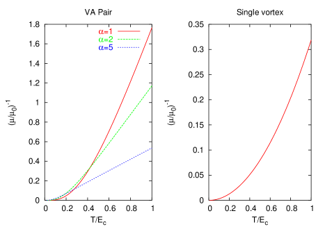
Figure 5: (Color online) Inverse mobility in units of $\mu_{0}^{-1}$ as a function of the rescaled temperature $T/E_{c}$. Left panel: inverse mobility of a vortex-antivortex pair, according to Eq. (81), at several values of $\alpha$. Right panel: inverse mobility of a single-vortex defect, according to Eq. (83)

V.2 Single vortex

Let us analyze now the behavior of the inverse mobility obtained when we identify the defect as a single vortex. In this case, instead of Eq. (79) the scattering potential reads

$$V_{1v}({\bf r})=\frac{1}{4}(\nabla\Psi_{1v})^{2}=\frac{1}{4r^{2}}.$$

As a consequence, the phase shifts defined by Eqs. (77) and (78) are given by ($m\geq 1$)

$$\delta_{m}=\arctan\frac{\pi}{8m}.$$ (82)

Note that the phase shifts in the case of a single-vortex do not depend on the wave-vector, but only on the angular momentum. Thus, the function $\mathcal{G}$ defined by Eq. (75), does not depend on the frequency

$$\mathcal{G}=\sum_{m=1}^{\infty}\frac{64\pi^{2}}{64\pi^{2}+[\pi^{2}+64m(m+1)]^{2}}\approx 0.032.$$

Because $\cal G$ is a constant, we can introduce the rescaled variable $y\equiv\hbar\xi/k_{B}T$ into the expression (69) for the inverse mobility, which yields

$$\mu^{-1}(T)=\mu_{0}^{-1}\frac{8\pi}{3}{\cal G}\left(\frac{T}{E_{c}}\right)^{2}.$$ (83)

Here, we used the fact that $\int_{0}^{\infty}dyy^{2}/(e^{y}-1)^{2}=\pi^{2}/3$. In comparison with the case of a vortex-antivortex pair, the main difference is that here the inverse mobility depends on the square of the temperature, for all the temperatures. In the right panel of Fig. 5 we plot $(\mu/\mu_{0})^{-1}$ as a function of $T/E_{c}$: notice that the overall variation of the inverse mobility is smaller compared to the case of the vortex-antivortex pair, but they are still of the same order of magnitude.

VI Application of the model: the case of cuprates

VI.1 The spiral state in cuprates

Although the model we have developed above could be applied to describe the dynamics of topological defects in several frustrated Heisenberg spin systems, here we concentrate on lightly doped cuprates. Indeed, a large part of the literature devoted to frustrated spin systems is connected to the $t-J$ model, which is the strong-coupling limit of the Hubbard model. The latter is considered to be the prototype of an effective description of the CuO₂ planes of cuprate superconductors. At half-filling the $t-J$ model describes a spin-$1/2$ antiferromagnet which is believed to have long-range order at zero temperature. As the system is doped away from half-filling the motion of a hole will leave a trail of spins pointing in the wrong direction. Thus, two issues must be settled: (i) the character of the quasiparticle wave function and (ii) the effect of the hole motion on the spin background. Both issues have been extensively addressed in the literature. In the atomic limit ($t=J=0$) of the Hubbard model, considered by Brinkman and Rice, brinkman the “string” of perturbed spins can be healed only by retracing the original path and returning all the spins to their original position. As a consequence, in the presence of a finite but small $J$, they argued that the ground state of the hole involves a magnetic polaron: the cost of creating a ferromagnetic region around the hole is compensate by the fact that inside this ferromagnetic cloud it can sit at the free-particle band edge.

At larger value of $J$ ($1\gtrsim J/t\gtrsim 5\times 10^{-3}$) Shraiman and Siggia siggia881 showed that at least in the Ising limit ($J_{z}\neq 0,J_{\perp}=0$) the picture of band narrowing effect is more appropriate than the polaron formation. In the Ising limit the holes are infinitely massive, because they are self-trapped to their original position by the “string” of overturned spins. When a finite $J_{\perp}$ is included, quantum spin fluctuations associated with it can repair a pair of overturned spins and the mass of the holes becomes large but finite.trugman Several calculations schmitt ; kane ; fulde were performed using an effective Hamiltonian which couples the holes (constrained to no double occupancy) to Holstein-Primakoff spin-waves. The result is that the hole moves on a given sublattice, forming a narrow ($\sim J$) quasiparticle band with the minimum at the wave-vector $(\pm\pi/2,\pm\pi/2)$, plus an incoherent part originating from the spin-wave excitations created by the hole motion. By using a semiclassical approach, Shraiman and Siggia siggia881 ; siggia882 ; siggia89 showed that one can assign to the hole states a dipolar momentum ${\bf p}_{a}$, which is a vector both in lattice and spin space. The coupling between this dipolar moment and the magnetization current ${\bf j}_{a}={\bf\Omega}\times\partial_{a}{\bf\Omega}$ of the antiferromagnetic background, described by a NL$\sigma$ model for ${\bf\Omega}$, leads, at finite doping, to a spiral re-ordering of the antiferromagnetic phase of the background spins. Within a similar approach, Gooding gooding has argued that a strong localization of the hole could eventually lead to a skyrmion-like configuration of the background spins. However, while the polaron or the skyrmion formation seem to be plausible scenarios for a single defect, at finite doping the picture proposed by Shraiman and Siggia of a new helical spin configuration is more likely. Later, many calculations on the $t-J$ (or $t-t^{\prime}-J$) model based on different approaches have indeed confirmed that a spiral ground state can be favorable at low doping. kane90 ; schulz ; mori ; weng ; kotov

Recently, the interest on spiral formation in $t-J$-based models has been revived due to the experimental observation of incommensurate spin correlations in cuprates, i.e., an enhancement of the spin susceptibility at a wave vector ${\bf k}_{s}$ slightly displaced with respect to the commensurate wave vector $(\pi/a,\pi/a)$. In particular, detailed measurements of the incommensurability as a function of doping are available for lanthanum-based compounds. NSSG ; antonio For doping $x$ larger than $0.05$, i.e., in the regime where the samples are superconducting, the observation of four peaks at $(\pi/a\pm\delta,\pi/a)$ and $(\pi/a,\pi/a\pm\delta)$, and the simultaneous measurement of incommensurate charge peaks, lead to a natural interpretation of the spin incommensurability in terms of antiferromagnetic domains separated by charge stripes oriented along the principal axis.tran ; zaanen ; yama However, at lower doping, for $0.02<x<0.05$, in the so-called spin-glass regime, where no superconductivity is observed, only two diagonal peaks have been measured,NSSG similar to the ones represented in Fig. 1. Even though these peaks could still arise from diagonal charge stripe formation, several arguments suggest that a spiral picture in this regime is more likely, as discussed in Refs. antonio, ; nils, ; kotov, .

These observations stimulated further investigations on the microscopic derivation of the $SO(3)$ NL$\sigma$ model (II), which can allow for the determination of the various microscopic parameters. Klee and Muramatsuklee considered the continuum field theory arising from a microscopic spin-fermion model, where itinerant electrons are coupled via a Kondo-like interaction to localized spins, described by the Heisenberg model. The spin-fluctuations around the spiral configuration (1) are included by allowing the vectors ${\bf n}_{1}$ and ${\bf n}_{2}$ to vary slowly on the lattice scale, and by adding a small ferromagnetic frustration ${\bf L}$, which is afterward integrated out,

$$\frac{\bf S}{S}=\frac{{\bf n}+a{\bf L}}{\sqrt{1+2a{\bf n}\cdot{\bf L}+a^{2}{\bf L}^{2}}}.$$

By also taking into account the coupling to the fermions and integrating them out, Klee and Muramatsu derived an effective action for the spin field which is the $SO(3)$ NL$\sigma$ model (II) with an additional term

$${\cal S}^{KM}=\int dtd^{2}{\bf x}[\kappa_{k}(\partial_{t}{\bf n}_{k})^{2}-p_{k\alpha}\left(\partial_{\alpha}{\bf n}_{k}\right)^{2}]$$

$$-\int dtd^{2}{\bf x}s_{\alpha}\left({\bf n}_{1}\cdot\partial_{\alpha}{\bf n}_{2}\right).$$ (84)

In the above action both the exchange $J$ between the spins and the fermionic susceptibilities contribute to the coupling constants $\kappa$ and $p_{\alpha}$. If only the Heisenberg interaction between the spins is considered, then $\kappa_{1}=\kappa_{2}\equiv\kappa=1/\{8Ja^{2}[2+\sum_{\alpha}\cos(Q_{\alpha}a)]\}$, $\kappa_{3}\simeq 0$, $p_{1\alpha}=p_{2\alpha}=(JS^{2}/4)\cos(Q_{\alpha}a)$, $p_{3\alpha}\simeq 0$ and $s_{\alpha}=(JS^{2}/a)\sin(Q_{\alpha}a)$. The subtle interplay between holes and spins is represented in the last term of the microscopically derived effective model (84). Indeed, since it is not positive definite, the weight of some field configurations in the path integral will tend to infinity, hence leading to instabilities. In order to ensure the action to be at a minimum, one should impose the condition that the full coefficients $s_{\alpha}=\chi_{\alpha}-(JS^{2}/a)\sin(Q_{\alpha}a)$, where $\chi_{\alpha}$ is the holes’ contribution, must vanish. This stability argument determines the spiral incommensurability $Q_{\alpha}$ as a function of the microscopic parameters and the doping concentration.klee

A more general derivation of the stability condition has been proposed recently by Hasselmann et al.nils In this approach, Eq. (84) is considered as the continuum limit of the Heisenberg model alone and the effect of doping is included within a minimum coupling of the order parameter to a gauge field $\bf B_{\alpha}$ representing the dipolar character of the hole state, already emphasized by Shraiman and Siggia. siggia881 ; siggia882 ; siggia89 It is then shown that the stability condition

$$p_{k\alpha}\partial_{\alpha}{\bf n}_{k}\cdot[{\bf B}_{\alpha}]_{D}\times{\bf n}_{k}+s_{\alpha}{\bf n}_{1}\cdot\partial_{\alpha}{\bf n}_{2}=0,$$

where $[{\bf B}_{\alpha}]_{D}$ denotes the ordered fraction of dipoles, relates the incommensurate vector ${\bf Q}$ to the hole density, nils in agreement with neutron scattering measurements in lanthanum cuprates.NSSG Moreover, the dipolar frustration described within this minimal-coupling scheme renormalizes the bare coefficients $p_{k\alpha}$ of Eq. (84) leading the system toward a stable fixed point where $p_{1\alpha}=p_{2\alpha}=p_{3\alpha}\equiv p_{\alpha}$,nils which corresponds to the model (2) that we considered. In this picture we can also determine the parameter $\kappa=JS^{2}/4c^{2}$, where $c=\sqrt{c_{\parallel}c_{\perp}}\approx 2\sqrt{2}JSa$ and $(c_{\parallel}/c_{\perp})^{2}=\cos(Qa)$.nils As a consequence, we can now apply our previous results to the spin-glass phase of lanthanum cuprates.

VI.2 Inverse mobility in cuprates

Until now we evaluated the inverse mobility of the defect without specifying how this quantity can be accessed experimentally. As we explained above, in lightly doped cuprates the holes act at the same time as source and stabilizing mechanism of the dipolar frustration. When topological defects are present in the spiral spin texture, one could expect that the holes sit on top of the defects (single vortex or vortex-antivortex pair) to minimize the frustration. Thus, the measured in-plane inverse mobility of the holes would be described by Eq. (69) with the damping coefficient given by Eq. (76). However, this scenario should apply only for temperatures above $150$ K, because below this temperature the experiments signal charge localization.

In the case of cuprates, the magnon temperature $E_{c}$ is the antiferromagnetic coupling $J\approx 1200$ K measured at zero doping. Actually, a lower value is expected, if one takes into account the renormalization of the spin-spin interaction due to the disorder introduced by hole doping and quantum effects. The resulting inverse mobility as a function of temperature for the case of a vortex-antivortex pair is reported in Fig. 6 for several values of $E_{c}$ and $\alpha$. Observe that using $a=3.8\AA$, as appropriate for cuprates, one obtains $\mu_{0}^{-1}=0.46$ Vs/cm². Inspection of Fig. 6 shows that already at $E_{c}=1000$ K the overall variation of $\mu^{-1}$ between 150 K and 300 K is of order of $0.05$ Vs/cm², as observed experimentally. ando Moreover, in the case of the vortex-antivortex pair, an upper limit for the application of Eq. (81) is given by the temperature $T_{v}$ of the vortex-antivortex unbinding. By estimating $T_{v}\sim\pi JS^{2}/2$, in analogy with the $XY$ model, we find that $T_{v}$ is of order of 400 K for the values of $E_{c}$ used in Fig. 6.

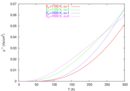
Figure 6: (Color online) Contribution (81) of the motion of a vortex-antivortex pair to the inverse mobility of the holes in cuprates.

The inverse mobility of a single defect is shown in Fig. 7. The overall variation of the inverse mobility turns out to be quantitatively smaller in this case. As we explained in the previous section, the main difference between the temperature dependence of the inverse mobility obtained with the single vortex or with the vortex-antivortex pair is that in the former case $\mu^{-1}\propto T^{2}$ always, while in the latter case $\mu^{-1}$ evolves towards a linear behavior at a crossover temperature which depends on $E_{c}$ and $\alpha$. As we discussed in Sec. II, the presence of the two kinds of defects depends on their energy, which scales as $E[\Psi_{1v}]\sim\ln\xi$ for the single vortex and $E[\Psi_{2v}]\sim\ln d$ for the pair, where $\xi$ is the correlation length and $d$ the distance between vortices, respectively. In the absence of disorder and at low temperatures, one would expect $\xi$ to be finite, but still large enough to prevent the formation of free defects below the crossover temperature $T_{v}$, where pairs start to unbind. kawamura1 ; southern ; wintel2 ; caffarel However, in Ref. nils, it has been argued that disorder leads to a strong reduction of the correlation length, and thus single defects start to proliferate already at temperatures lower than $T_{v}$. Comparison with recent resistivity data seems to support this conclusion. Indeed, studies performed by Ando et al.ando1 for compounds in the spin-glass regime indicate that the second derivative of the in-plane resistivity with respect to the temperature is positive up to $\sim 300K$, implying that $\rho_{ab}\sim T^{\eta}$ with $\eta>1$. Based on previous experiments,ando we interpreted the resistivity data for cuprates in terms of the dissipative motion of vortex-antivortex pairs only, which gives rise to a linear resistivity.juricic However, in the light of these new data, one could speculate about the coexistence of single-vortices and vortex-antivortex pairs, which would consequently lead to a power-law behavior of the resistivity with a more complicated exponent, expected to be larger than one.

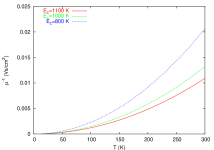
Figure 7: (Color online) Contribution (81) of the motion of a single-vortex defect to the inverse mobility of the holes in cuprates.

VII Conclusions

We study here the properties of frustrated Heisenberg spin systems in which a noncollinear spin state is formed at low temperatures. In the long-wavelength limit, the system is described by the $SO(3)$ NL$\sigma$ model, and several differences arise with respect to the usual $O(3)$ NL$\sigma$ model adopted to describe collinear spin states. In particular, vortex-like excitations play a crucial role in determining the finite-temperature critical behavior.azaria We concentrated on the contribution of these topological defects to transport properties. Our approach extends to a non-Abelian field theory the well-known collective-coordinate method employed previously to study the dissipative mechanism in one- and two-dimensional systems. amir We consider two kinds of topological defects: a single vortex and a vortex-antivortex pair. We show that the interaction between the defect and the spin waves is described by a particle coupled to a bath of harmonic oscillators. The scattering of the defect by the magnons leads to its dissipative motion. We integrated out the bath and calculated the mobility of the defect. Quite generally, its temperature dependence is determined by the thermal activation of the magnons, which vanishes at zero temperature and follows, at higher temperatures, a power law whose exponent depends on the type of defect. In particular, we find that it is linear for the vortex-antivortex pair and quadratic for the single vortex. We apply the model to describe transport in lightly doped lanthanum cuprates. Several theoretical and experimental studies suggest that in these systems a spiral state is formed at low temperatures.nils ; NSSG ; juricic ; ando Our results for the mobility indicate indeed that a possible mechanism for transport in these materials, for 150K$<T<$400K, could be the dissipative motion of an electrical charge attached to a single vortex or a vortex-antivortex topological defect.

Although we have applied the model to the particular case of lightly doped cuprates, the approach presented here is quite general, and can be employed to investigate the role of topological defects in any frustrated spin system described by the $SO(3)$ NL$\sigma$ model. As far as the spin-glass phase of cuprate superconductors is concerned, the incommensurate peaks, the value of the resistivity, as well as its linear temperature dependence and anisotropy, might be explained within both the spiral and the stripe model.nils ; NSSG ; juricic ; ando A theoretical prediction that would discriminate between these two scenarios, as well as its experimental realization, are still missing. This issue is currently under investigation. barbosa

VIII Acknowledgments

We would like to acknowledge fruitful discussions with N. Hasselmann, A. H. Castro Neto, A. V. Ferrer and M. B. Silva Neto. This work was supported by the projects 620-62868.00 and MaNEP (9,10,18) of the Swiss National Foundation for Scientific Research. A.O.C. wishes to thank the partial support of Conselho Nacional de Desenvolvimento Científico e Tecnológico (CNPq) and Fundação de Amparo à Pesquisa no Estado de São Paulo (FAPESP).

Appendix A Energy of a single vortex and of a vortex-antivortex pair

In this appendix we will calculate the energy of the topological defects in the $SO(3)$ NL$\sigma$ model. Static solutions of the model obey the Laplace equation

$$\nabla^{2}\Psi({\bf r})=0.$$ (85)

A single-vortex solution centered at ${\bf R}=(X,Y)$ has the form

$$\Psi_{1v}({\bf r},{\bf R})=\arctan\left(\frac{x-X}{y-Y}\right).$$ (86)

Its energy is given by

$$E[\Psi_{1v}]=\mathcal{N}c^{2}\int d^{2}{\bf r}(\nabla\Psi_{1v})^{2}=2\pi\mathcal{N}c^{2}\ln\frac{\ell}{a}.$$

A bound vortex-antivortex pair described by

$$\Psi_{2v}=\Psi_{1v}({\bf r},{\bf R}_{1})-\Psi_{1v}({\bf r},{\bf R}_{2}),$$ (87)

with $\Psi_{1v}$ given by Eq. (86), is also a solution of Eq. (85). The vortex-antivortex defect can be written in a more compact form as

$$\Psi_{2v}=\arctan\left\{\frac{[{\bf d}\times({\bf r}-{\bf R})]_{z}}{({\bf r}-{\bf R})^{2}-{\bf d}^{2}/4}\right\},$$

where the center of mass and relative coordinate, respectively, are given by

$${\bf R}=\frac{1}{2}({\bf R}_{1}+{\bf R}_{2}),\qquad{\bf d}={\bf R}_{2}-{\bf R}_{1}.$$

In order to evaluate the energy of the vortex-antivortex pair

$$E[\Psi_{2v}]=\mathcal{N}c^{2}\int d^{2}{\bf r}(\nabla\Psi_{2v})^{2},$$

we use Eq. (87), which yields

$$E[\Psi_{2v}]=\mathcal{N}c^{2}(I_{11}+I_{22}-2I_{12}),$$ (88)

where

$$I_{jj^{\prime}}\equiv\int d^{2}{\bf r}(\nabla\Psi^{(j)})(\nabla\Psi^{(j^{\prime})}).$$

and $\Psi^{(1,2)}\equiv\Psi_{1v}({\bf r},{\bf R}_{(1,2)})$. It is easy to show that $I_{11}$ and $I_{22}$ are equal,

$$I_{11}=I_{22}=2\pi\ln\frac{\ell}{a}.$$ (89)

The integral $I_{12}$ is highly non-trivial. After some calculations, it can be expressed in the form

$$I_{12} = \frac{1}{2}\int d^{2}{\bf r}\frac{1}{({\bf r}-{\bf R}_{1})^{2}}+\frac{1}{2}\int d^{2}{\bf r}\frac{1}{({\bf r}-{\bf R}_{2})^{2}}$$ (90)

$$- \frac{1}{2}({\bf R}_{1}-{\bf R}_{2})^{2}\int d^{2}{\bf r}\frac{1}{({\bf r}-{\bf R}_{1})^{2}({\bf r}-{\bf R}_{2})^{2}}.$$

The first two integrals on the right hand side of Eq. (90) are identical and equal to $I_{11}$, whereas the last one must be evaluated separately. Let us denote it as $I_{12}^{(3)}$. After regularization, it becomes

$$I_{12}^{(3)}=\int d^{2}{\bf r}\frac{1}{[({\bf r}-{\bf R}_{1})^{2}+a^{2}][({\bf r}-{\bf R}_{2})^{2}+a^{2}]}.$$

By introducing new coordinates with ${\bf r}-{\bf R}_{2}\rightarrow{\bf r}$, the last integral acquires the form

$$I_{12}^{(3)}=\int d^{2}{\bf r}\frac{1}{[{\bf r}^{2}+a^{2}][({\bf r}+{\bf d})^{2}+a^{2}]}.$$ (91)

In order to simplify Eq. (91), we introduce polar coordinates $x=r\cos\varphi,y=r\sin\varphi$

$$I_{12}^{(3)}=\int_{0}^{\ell}dr\frac{r}{r^{2}+a^{2}}\int_{0}^{2\pi}\frac{d\varphi}{r^{2}+2rd\cos(\varphi-\phi)+d^{2}+a^{2}},$$

where $(d,\phi)$ are polar coordinates of ${\bf d}$. Integrating over the angle $\varphi$, we obtain

$$I_{12}^{(3)}=\int_{0}^{\ell}dr\frac{r}{r^{2}+a^{2}}\frac{2\pi}{\sqrt{(r^{2}-d^{2})^{2}+2a^{2}(r^{2}+d^{2})+a^{4}}}.$$

After substituting $u=1/(r^{2}+a^{2})$, the above integral reads

$$I_{12}^{(3)}=\pi\int_{1/a^{2}}^{1/(\ell^{2}+a^{2})}\frac{du}{\sqrt{u^{2}d^{2}(d^{2}+2a^{2})-2ud^{2}+1}}.$$

Straightforward calculations give

$$I_{12}^{(3)} = \frac{\pi}{d\sqrt{d^{2}+2a^{2}}}\ln\left\{\frac{1}{4a^{4}}\left[d^{3}+\sqrt{d^{6}+8a^{6}}\right]\right.$$ (92)

$$\left.\left[d+\sqrt{d^{2}+2a^{2}}\right]\right\}\approx\frac{4\pi}{d\sqrt{d^{2}+2a^{2}}}\ln\frac{d}{a}.$$

Substitution of Eq. (92) into Eq. (90) yields

$$I_{12}=2\pi\left[\ln\frac{\ell}{a}-\frac{d}{\sqrt{d^{2}+2a^{2}}}\ln\frac{d}{a}\right].$$ (93)

After inserting the last relation together with Eq. (89) into Eq. (88), we finally obtain the energy of the vortex-antivortex pair

$$E[\Psi_{2v}]=\frac{4\pi d}{\sqrt{d^{2}+2a^{2}}}\mathcal{N}c^{2}\ln\frac{d}{a}\approx 4\pi\mathcal{N}c^{2}\ln\frac{d}{a},$$ (94)

which shows that the energy of the defect pair is finite.

Appendix B Dynamics of the fluctuations around the defect

Using the identities

$$\sigma^{a}\sigma^{b} = \delta^{ab}+i\epsilon^{abc}\sigma^{c},$$

$$\exp\left(\frac{i}{2}\vec{\sigma}\cdot\vec{\alpha}\right) = \cos\frac{\alpha}{2}+i\frac{\vec{\sigma}\cdot\vec{\alpha}}{\alpha}\sin\frac{\alpha}{2},$$

where $\alpha\equiv|\vec{\alpha}|$, together with Eq. (12), one can show that

$$\partial_{\mu}g_{s} = \frac{i}{2}m^{a}\sigma^{a}g_{s}\partial_{\mu}\Psi_{v},$$ (95)

$$\partial_{\mu}g_{\varepsilon} = \frac{i}{2}\frac{\vec{\sigma}\cdot\vec{\varepsilon}}{\varepsilon}\partial_{\mu}\varepsilon g_{\varepsilon}+\frac{i\sigma^{a}}{\varepsilon}\left[\partial_{\mu}\varepsilon^{a}-\frac{\varepsilon^{a}(\vec{\varepsilon}\cdot\partial_{\mu}\vec{\varepsilon})}{\varepsilon^{2}}\right]\sin\frac{\varepsilon}{2}.$$

Here $\varepsilon$ stands for $|\vec{\varepsilon}|$. By inserting Eqs. (95) into the field $A_{\mu}^{a}$ given by (3), we obtain

$$A_{\mu}^{a}\equiv A_{\mu 1}^{a}+A_{\mu 2}^{a}+A_{\mu 3}^{a}+A_{\mu 4}^{a},$$ (96)

with

$$A_{\mu 1}^{a} = \frac{1}{4}{\rm tr}(\sigma^{a}g_{\varepsilon}^{-1}g_{s}^{-1}\sigma^{b}g_{s}g_{\varepsilon})m^{b}\partial_{\mu}\Psi_{v},$$

$$A_{\mu 2}^{a} = \frac{1}{2\varepsilon}{\rm tr}(\sigma^{a}g_{\varepsilon}^{-1}\sigma^{b})\partial_{\mu}\varepsilon^{b}\sin\frac{\varepsilon}{2},$$

$$A_{\mu 3}^{a} = -\frac{1}{2}{\rm tr}(\sigma^{a}g_{\varepsilon}^{-1}\sigma^{b})\frac{\varepsilon^{b}(\vec{\varepsilon}\cdot\partial_{\mu}\vec{\varepsilon})}{\varepsilon^{3}}\sin\frac{\varepsilon}{2},$$

$$A_{\mu 4}^{a} = \frac{1}{4\varepsilon}{\rm tr}(\sigma^{a}g_{\varepsilon}^{-1}\sigma^{b}\partial_{\mu}\varepsilon g_{\varepsilon})\varepsilon^{b}.$$

The parameter $\varepsilon$ is small, $\varepsilon\ll 1$, because $g_{\varepsilon}$ describes fluctuations around the defect. Using the properties of the Pauli matrices, we find

$$g_{\varepsilon}=1+\frac{i}{2}\vec{\sigma}\cdot\vec{\varepsilon}-\frac{1}{8}\varepsilon^{2}+\mathcal{O}(\varepsilon^{3}),$$

which allows us to write

$$A_{\mu 1}^{a} = \frac{1}{4}{\rm tr}\left\{\sigma^{a}\left(\cos\frac{\Psi_{v}}{2}-i\vec{m}\cdot\vec{\sigma}\sin\frac{\Psi_{v}}{2}\right)\sigma^{b}\right.$$

$$\left.\left(\cos\frac{\Psi_{v}}{2}+i\vec{m}\cdot\vec{\sigma}\sin\frac{\Psi_{v}}{2}\right)\right\}m^{b}\partial_{\mu}\Psi_{v}\left(1-\frac{\varepsilon^{2}}{4}\right)$$

$$+ \frac{i}{8}{\rm tr}\left\{\sigma^{a}\left(\cos\frac{\Psi_{v}}{2}-i\vec{m}\cdot\vec{\sigma}\sin\frac{\Psi_{v}}{2}\right)\sigma^{b}\right.$$

$$\left.\left(\cos\frac{\Psi_{v}}{2}+i\vec{m}\cdot\vec{\sigma}\sin\frac{\Psi_{v}}{2}\right)(\vec{\sigma}\cdot\vec{\varepsilon})\right\}m^{b}\partial_{\mu}\Psi_{v}$$

$$- \frac{i}{8}{\rm tr}\left\{\sigma^{a}(\vec{\sigma}\cdot\vec{\varepsilon})\left(\cos\frac{\Psi_{v}}{2}-i\vec{m}\cdot\vec{\sigma}\sin\frac{\Psi_{v}}{2}\right)\right.$$

$$\left.\sigma^{b}\left(\cos\frac{\Psi_{v}}{2}+i\vec{m}\cdot\vec{\sigma}\sin\frac{\Psi_{v}}{2}\right)\right\}m^{b}\partial_{\mu}\Psi_{v}$$

$$+ \frac{1}{16}{\rm tr}\left\{\sigma^{a}(\vec{\sigma}\cdot\vec{\varepsilon})\left(\cos\frac{\Psi_{v}}{2}-i\vec{m}\cdot\vec{\sigma}\sin\frac{\Psi_{v}}{2}\right)\right.$$

$$\left.\sigma^{b}\left(\cos\frac{\Psi_{v}}{2}+i\vec{m}\cdot\vec{\sigma}\sin\frac{\Psi_{v}}{2}\right)(\vec{\sigma}\cdot\vec{\varepsilon})\right\}m^{b}\partial_{\mu}\Psi_{v}.$$

After some algebra, the last equation acquires the form

$$A_{\mu 1}^{a} = \frac{1}{2}m^{a}\partial_{\mu}\Psi_{v}\left(1-\frac{\varepsilon^{2}}{4}\right)+\frac{1}{2}\epsilon^{abc}\varepsilon^{b}m^{c}\partial_{\mu}\Psi_{v}$$ (97)

$$+ \frac{1}{4}\varepsilon^{a}\varepsilon^{b}m^{b}\partial_{\mu}\Psi_{v}-\frac{1}{8}\varepsilon^{2}m^{a}\partial_{\mu}\Psi_{v}+\mathcal{O}(\varepsilon^{3}).$$

Analogously, one can show that

$$A_{\mu 2}^{a} = \frac{1}{2}\partial_{\mu}\varepsilon^{a}+\mathcal{O}(\varepsilon^{3})$$

$$A_{\mu 3}^{a} = -\frac{\varepsilon^{a}(\vec{\varepsilon}\cdot\partial_{\mu}\vec{\varepsilon})}{\varepsilon^{2}}+\mathcal{O}(\varepsilon^{3})$$

$$A_{\mu 4}^{a} = \frac{\varepsilon^{a}}{2\varepsilon}\partial_{\mu}\varepsilon+\mathcal{O}(\varepsilon^{3}).$$ (98)

By substituting Eqs. (97) and (B) into the field $A_{\mu}^{a}$ given by (96), and retaining terms up to the second order in $\varepsilon$, we obtain

$$A_{\mu}^{a} = \frac{1}{2}m^{a}\partial_{\mu}\Psi_{v}\left(1-\frac{\varepsilon^{2}}{2}\right)+\frac{1}{4}\varepsilon^{a}\varepsilon^{b}m^{b}\partial_{\mu}\Psi_{v}$$ (99)

$$+ \frac{1}{2}\epsilon^{abc}\varepsilon^{b}m^{c}\partial_{\mu}\Psi_{v}+\frac{1}{2}\partial_{\mu}\varepsilon^{a}+\frac{1}{4}\epsilon^{abc}\varepsilon^{b}\partial_{\mu}\varepsilon^{c},$$

and

$$A_{\mu}^{a}A_{\mu}^{a} = \frac{1}{4}(\partial_{\mu}\Psi_{v})^{2}+\frac{1}{4}(\partial_{\mu}\vec{\varepsilon})^{2}+\frac{1}{2}m^{a}\partial_{\mu}\varepsilon^{a}\partial_{\mu}\Psi_{v}$$ (100)

$$+ \frac{1}{4}\epsilon^{abc}\partial_{\mu}\varepsilon^{a}\varepsilon^{b}m^{c}\partial_{\mu}\Psi_{v}.$$

Appendix C Evaluation of the kernel

In this appendix we will express the kernel $K$ defined by Eq. (40) as a functional integral. First, we divide the time interval $[0,t]$ into $(m-1)$ subintervals of length $\epsilon$, so $t=(m-1)\epsilon$, and use $(m-1)$ completeness relations between the $(m-1)$ exponential functions,

$$K({\bf x},\vec{\alpha}^{*};{\bf y},\vec{\beta};t)\equiv\langle{\bf x},\vec{\alpha}|e^{-\frac{i\hat{H}t}{\hbar}}|{\bf y},\vec{\beta}\rangle$$

$$= \int d^{2}{\bf x}_{m-1}...\int d^{2}{\bf x}_{1}\int\frac{d^{2}\vec{\zeta}_{m-1}}{\pi^{2N}}...\int\frac{d^{2}\vec{\zeta}_{1}}{\pi^{2N}}$$

$$\langle{\bf x}_{m}\vec{\zeta}_{m}|e^{-\frac{i\hat{H}\epsilon}{\hbar}}|{\bf x}_{m-1}\vec{\zeta}_{m-1}\rangle$$

$$\langle{\bf x}_{m-1}\vec{\zeta}_{m-1}|e^{-\frac{i\hat{H}\epsilon}{\hbar}}|{\bf x}_{m-2}\vec{\zeta}_{m-2}\rangle...\langle{\bf x}_{1}\vec{\zeta}_{1}|e^{-\frac{i\hat{H}\epsilon}{\hbar}}|{\bf x}_{0}\vec{\zeta}_{0}\rangle,$$

where

$${\bf x}_{m}\equiv{\bf x},\quad{\bf x}_{0}\equiv{\bf y}$$

$$\vec{\zeta}_{m}\equiv\vec{\alpha},\quad\vec{\zeta}_{0}\equiv\vec{\beta}.$$ (101)

By inserting $m$ completeness relations in the momentum representation into Eq. (C), we obtain

$$K({\bf x},\vec{\alpha}^{*};{\bf y},\vec{\beta};t)=\left(\prod_{k=1}^{m-1}d^{2}{\bf x}_{k}\frac{d^{2}\vec{\zeta}_{k}}{\pi^{2N}}\right)\left(\prod_{k=1}^{m}d^{2}{\bf P}_{k}\right)$$

$$\prod_{k=1}^{m}\langle{\bf x}_{k}\vec{\zeta}_{k}|e^{-\frac{i\hat{H}\epsilon}{\hbar}}|{\bf P}_{k}\vec{\zeta}_{k-1}\rangle\langle{\bf P}_{k}|{\bf x}_{k-1}\rangle.$$ (102)

The matrix element $\langle{\bf x}_{k}\vec{\zeta}_{k}|e^{-\frac{i\hat{H}\epsilon}{\hbar}}|{\bf P}_{k}\vec{\zeta}_{k-1}\rangle$, $(k=1,...,m)$, can be evaluated using that $\epsilon\ll t$. It reads

$$\langle{\bf x}_{k}\vec{\zeta}_{k}|e^{-\frac{i\hat{H}\epsilon}{\hbar}}|{\bf P}_{k}\vec{\zeta}_{k-1}\rangle=\langle{\bf x}_{k}|{\bf P}_{k}\rangle\langle\vec{\zeta}_{k}|\vec{\zeta}_{k-1}\rangle$$

$$\exp\left[-\frac{i\epsilon}{\hbar}H({\bf x}_{k},{\bf P}_{k};\vec{\zeta}_{k}^{*},\vec{\zeta}_{k-1})\right],$$ (103)

where

$$H({\bf x}_{k},{\bf P}_{k};\vec{\zeta}_{k}^{*},\vec{\zeta}_{k-1})\equiv\frac{\langle{\bf x}_{k}\vec{\zeta}_{k}|\hat{H}|{\bf P}_{k}\vec{\zeta}_{k-1}\rangle}{\langle{\bf x}_{k}|{\bf P}_{k}\rangle\langle\vec{\zeta}_{k}|\vec{\zeta}_{k-1}\rangle}.$$

Substituting the matrix element given by Eq.  (C) into Eq. (C), recalling that

$$\langle{\bf P}|{\bf x}\rangle=\frac{1}{2\pi\hbar}\exp\left(-\frac{i}{\hbar}{\bf P}\cdot{\bf x}\right),$$

and using the properties of the overlap of coherent states, we find that the kernel acquires the form

$$K({\bf x},\vec{\alpha}^{*};{\bf y},\vec{\beta};t)=\int\frac{d^{2}{\bf P}_{m}}{2\pi\hbar}\left(\prod_{l=1}^{m-1}\int\frac{d^{2}{\bf x}_{l}d^{2}{\bf P}_{l}}{2\pi\hbar}\frac{d^{2}{\vec{\zeta}}_{l}}{\pi^{2N}}\right)$$ (104)

$$\exp\left\{\sum_{k=1}^{m}\frac{1}{2}\left[\vec{\zeta}_{k-1}\cdot(\vec{\zeta}^{*}_{k}-\vec{\zeta}^{*}_{k-1})-\vec{\zeta}^{*}_{k}\cdot(\vec{\zeta}_{k}-\vec{\zeta}_{k-1})\right]\right.$$

$$+ \left.\frac{i}{\hbar}\left[{\bf P}_{k}({\bf x}_{k}-{\bf x}_{k-1})-\epsilon H({\bf x}_{k},{\bf P}_{k};\vec{\zeta}_{k}^{*},\vec{\zeta}_{k-1})\right]\right\}.$$

In order to integrate over the momenta ${\bf P}_{k}$, we have to explicitly calculate $H({\bf x}_{k},{\bf p}_{k};\vec{\zeta}_{k}^{*},\vec{\zeta}_{k-1})$. Using the coherent state representation for the bath of harmonic oscillators, we find

$$H({\bf x}_{k},{\bf P}_{k};\vec{\zeta}_{k}^{*},\vec{\zeta}_{k-1})=\frac{{\bf P}_{k}^{2}}{2M}+\sum_{nm,i=a,b}\hbar\omega_{nm}\zeta_{nm,i}^{k*}\zeta_{nm,i}^{k-1}$$

$$- \frac{{\bf P}_{k}}{M}\sum_{nm,pq}\left[{\bf D}_{nm,pq}\zeta_{pq,a}^{k*}\zeta_{nm,a}^{k-1}-{\bf D}_{pq,nm}\zeta_{nm,b}^{k-1}\zeta_{pq,b}^{k*}\right],$$

which, after insertion into Eq. (104) and integration over the momenta ${\bf P}_{k}$, yields

$$K({\bf x},\vec{\alpha}^{*};{\bf y},\vec{\beta};t)=\left(\frac{M}{2i\pi\hbar}\right)^{m/2}\left(\prod_{l=1}^{m-1}\frac{d^{2}{\bf x}_{l}}{2\pi\hbar}\frac{d^{2}{\vec{\zeta}}_{l}}{\pi^{2N}}\right)$$ (105)

$$\exp\left\{\sum_{k=1}^{m}\frac{1}{2}\left[\vec{\zeta}_{k-1}(\vec{\zeta}^{*}_{k}-\vec{\zeta}^{*}_{k-1})-\vec{\zeta}^{*}_{k}(\vec{\zeta}_{k}-\vec{\zeta}_{k-1})\right]\right.$$

$$\left.-\frac{i\epsilon}{\hbar}\sum_{nm,i}\hbar\omega_{nm}\zeta_{nm,i}^{k*}\zeta_{nm,i}^{k-1}+\frac{iM\epsilon}{2\hbar}\left({\bf h}_{k}+\frac{{\bf x}_{k}-{\bf x}_{k-1}}{\epsilon}\right)^{2}\right\},$$

with

$${\bf h}_{k}\equiv\frac{\hbar}{M}\sum_{nm,pq}\left({\bf D}_{nm,pq}\zeta_{pq,a}^{k*}\zeta_{nm,a}^{k-1}-{\bf D}_{pq,nm}\zeta_{nm,b}^{k-1}\zeta_{pq,b}^{k*}\right).$$

Now, we consider the continuum limit, $\epsilon\to 0$, of the last equation. Using the boundary conditions (C), the first term in the exponential in (105) becomes

$$\exp\left\{\sum_{k=1}^{m}\frac{1}{2}\left[\vec{\zeta}_{k-1}\cdot(\vec{\zeta}^{*}_{k}-\vec{\zeta}^{*}_{k-1})-\vec{\zeta}^{*}_{k}\cdot(\vec{\zeta}_{k}-\vec{\zeta}_{k-1})\right]\right\}$$

$$= \exp\left\{\frac{1}{2}\sum_{k=0}^{m-1}\vec{\zeta}_{k}\cdot(\vec{\zeta}_{k+1}^{*}-\vec{\zeta}_{k}^{*})-\frac{1}{2}\sum_{k=1}^{m}\vec{\zeta}_{k}^{*}\cdot(\vec{\zeta}_{k}-\vec{\zeta}_{k-1})\right\}$$

$$= \exp\left\{\frac{1}{2}[\vec{\zeta}_{0}\cdot(\vec{\zeta}_{1}^{*}-\vec{\zeta}_{0}^{*})-\vec{\zeta}_{m}^{*}\cdot(\vec{\zeta}_{m}-\vec{\zeta}_{m-1})]\right\}$$

$$\exp\left\{\frac{1}{2}\sum_{k=1}^{m-1}[\vec{\zeta}_{k}\cdot(\vec{\zeta}_{k+1}^{*}-\vec{\zeta}_{k}^{*})-\vec{\zeta}_{k}^{*}\cdot(\vec{\zeta}_{k}-\vec{\zeta}_{k-1})]\right\}$$

$$\rightarrow \exp\left(-\frac{1}{2}|\vec{\beta}|^{2}-\frac{1}{2}|\vec{\alpha}|^{2}\right)\exp\left\{\frac{1}{2}\vec{\beta}\cdot\vec{\zeta}^{*}(0)+\frac{1}{2}\vec{\alpha}^{*}\cdot\vec{\zeta}(t)\right\}$$

$$\exp\left\{\frac{1}{2}\int_{0}^{t}dt^{\prime}(\vec{\zeta}\cdot\dot{\vec{\zeta}^{*}}-\vec{\zeta}^{*}\cdot\dot{\vec{\zeta}})\right\}.$$

The other terms in Eq. (105) can be trivially written in the continuum limit, yielding then Eq. (41).

Appendix D Initial density matrix for the bath in the coherent state representation

It remains to evaluate the matrix elements of the initial density matrix for the bath in the coherent state representation

$$\rho_{B}({\vec{\beta}}^{*},{\vec{\beta}}^{\prime},0)=\langle{\vec{\beta}|\hat{\rho}_{B}(0)|{\vec{\beta}}^{\prime}}\rangle$$

with

$$\hat{\rho}_{B}(0)=\frac{1}{Z}\prod_{pq}e^{-U\omega_{pq}(\hat{a}_{pq}^{\dagger}\hat{a}_{pq}+\hat{b}_{pq}^{\dagger}\hat{b}_{pq})},$$

where the partition function reads

$$Z\equiv{\rm tr}\left[e^{-U\sum_{pq}\omega_{pq}(\hat{a}_{pq}^{\dagger}\hat{a}_{pq}+\hat{b}_{pq}^{\dagger}\hat{b}_{pq})}\right]=\prod_{pq}\left(1-e^{-\frac{\hbar\omega_{pq}}{k_{B}T}}\right)^{-2}.$$

Since the baths $a$ and $b$ are not coupled, the total density matrix is the product

$$\rho_{B}({\vec{\beta}}^{*},{\vec{\beta}}^{\prime},0)=\rho_{B,a}({\vec{\beta}}_{a}^{*},{\vec{\beta}}^{\prime}_{a},0)\rho_{B,b}({\vec{\beta}}_{b}^{*},{\vec{\beta}}^{\prime}_{b},0)$$

of the density matrices $\rho_{B,a}$ and $\rho_{B,a}$ for the baths $a$ and $b$, respectively, given by

$$\rho_{B,a}({\vec{\beta}}_{a}^{*},{\vec{\beta}}^{\prime}_{a},0)=\frac{1}{Z_{a}}\prod_{pq}\langle\beta_{pq,a}|e^{-U\omega_{pq}\hat{a}_{pq}^{\dagger}\hat{a}_{pq}}|\beta^{\prime}_{pq,a}\rangle$$

for the bath $a$, and analogously for the bath $b$, with the partition function

$$Z_{b}=Z_{a}={\rm tr}\left[e^{-U\sum_{pq}\omega_{pq}(\hat{a}_{pq}^{\dagger}\hat{a}_{pq})}\right]=\prod_{pq}\left(1-e^{-\frac{\hbar\omega_{pq}}{k_{B}T}}\right)^{-1}.$$

We shall evaluate the previous matrix element by inserting two unity operators in the occupation number representation for the bath $a$ (in the following, to simplify notation we omit the index $a$ in the ${\vec{\beta}}$, ${\vec{\beta}}^{\prime}$ and ${\bar{n}}$)

$$\rho_{B,a}({\vec{\beta}}^{*},{\vec{\beta}}^{\prime},0) = \frac{1}{Z_{a}}\prod_{pq}\langle\beta_{pq}|e^{-U\omega_{pq}\hat{a}_{pq}^{\dagger}\hat{a}_{pq}}|\beta^{\prime}_{pq}\rangle$$

$$= \frac{1}{Z_{a}}\prod_{pq}\sum_{n_{pq},n^{\prime}_{pq}}\langle\beta_{pq}|n_{pq}\rangle$$

$$\langle n_{pq}|e^{-U\omega_{pq}\hat{a}_{pq}^{\dagger}\hat{a}_{pq}}|n^{\prime}_{pq}\rangle\langle n^{\prime}_{pq}|\beta^{\prime}_{pq}\rangle.$$

Now, we use the scalar product of the states which define the coherent state and occupation number representations

$$\langle\beta_{pq}|n_{pq}\rangle=\frac{(\beta^{*}_{pq})^{n_{pq}}}{\sqrt{n_{pq}!}}e^{-\frac{|\beta_{pq}|^{2}}{2}}.$$

Substituting the above expression into Eq. (D), we obtain

$$\rho_{B,a}({\vec{\beta}}^{*},{\vec{\beta}}^{\prime},0) = \frac{1}{Z_{a}}\prod_{nm}\exp\left(-\frac{|\beta_{pq}|^{2}}{2}-\frac{|\beta^{\prime}_{pq}|^{2}}{2}\right)$$ (107)

$$\sum_{n_{pq}}\frac{1}{n_{pq}!}\left\{\exp\left(-\frac{\hbar\omega_{pq}}{k_{B}T}\right)\beta^{*}_{pq}\beta^{\prime}_{pq}\right\}^{n_{pq}}$$

$$= \frac{1}{Z_{a}}\prod_{pq}\exp\left(-\frac{|\beta_{pq}|^{2}}{2}-\frac{|\beta^{\prime}_{pq}|^{2}}{2}\right)$$

$$\exp\left[\beta^{*}_{pq}\beta^{\prime}_{pq}\exp(-U\omega_{pq})\right].$$

Appendix E Equations of motion

Our next step is to solve equations of motion (III.2). In order to achieve this aim, we introduce the ansatz

$$\zeta_{nm}(\tau) = e^{-i\omega_{nm}\tau}[\beta_{nm}+\sum_{kl\neq nm}W_{nm,kl}(\tau)\beta_{kl}],$$

$$\zeta^{*}_{nm}(\tau) = e^{i\omega_{nm}\tau}[\alpha^{*}_{nm}e^{-i\omega_{nm}t}$$ (108)

$$+ \sum_{kl\neq nm}\tilde{W}_{nm,kl}(\tau)e^{-i\omega_{kl}t}\alpha^{*}_{kl}],$$

where the functionals $W$ and $\tilde{W}$ will be determined from the equations of motion and $0\leq\tau\leq t$. By substituting the first time derivative of Eqs. (E) into the equations of motion (III.2), we obtain the expressions which determine the time evolution of the functionals $W$ and $\tilde{W}$

$$\dot{W}_{nm,kl}=W^{0}_{nm,kl}+\sum_{pq}W^{0}_{nm,pq}W_{pq,kl},$$

$$\dot{\tilde{W}}_{nm,kl}=-\tilde{W}^{0}_{nm,kl}-\sum_{pq}\tilde{W}^{0}_{nm,pq}\tilde{W}_{pq,kl},$$

with

$$W^{0}_{nm,kl}[{\bf x},\tau] = i\dot{{\bf x}}{\bf D}_{kl,nm}e^{i(\omega_{nm}-\omega_{kl})\tau},$$

$$\tilde{W}^{0}_{nm,kl}[{\bf x},\tau] = i\dot{{\bf x}}{\bf D}_{nm,kl}e^{-i(\omega_{nm}-\omega_{kl})\tau}.$$ (109)

Notice that $\tilde{W}^{0}_{nm,kl}=-W^{0*}_{nm,kl}$. Because $W$ and $\tilde{W}$ must satisfy the boundary conditions $W({\bf x},0)=0$ and $\tilde{W}({\bf x},t)=0$, we have

$$W_{nm,kl}[{\bf x},\tau] = \int_{0}^{\tau}dt^{\prime}W^{0}_{nm,kl}[{\bf x},t^{\prime}]$$

$$+ \sum_{pq}\int_{0}^{\tau}dt^{\prime}W^{0}_{nm,pq}[{\bf x},t^{\prime}]W_{pq,kl}[{\bf x},t^{\prime}],$$

$$\tilde{W}_{nm,kl}[{\bf x},\tau] = \int_{\tau}^{t}dt^{\prime}\tilde{W}^{0}_{nm,kl}[{\bf x},t^{\prime}]$$

$$+ \sum_{pq}\int_{\tau}^{t}dt^{\prime}\tilde{W}^{0}_{nm,pq}[{\bf x},t^{\prime}]\tilde{W}_{pq,kl}[{\bf x},t^{\prime}],$$

which, using the Born approximation, acquires the form

$$W_{nm,kl}[{\bf x},\tau]=\int_{0}^{\tau}dt^{\prime}W_{nm,kl}^{0}[{\bf x},t^{\prime}]$$

$$+ \sum_{pq}\int_{0}^{\tau}dt^{\prime}W^{0}_{nm,pq}[{\bf x},t^{\prime}]\int_{0}^{t^{\prime}}dt^{\prime\prime}W^{0}_{pq,kl}[{\bf x},t^{\prime}],$$

$$\tilde{W}_{nm,kl}[{\bf x},\tau]=\int_{\tau}^{t}dt^{\prime}\tilde{W}_{nm,kl}^{0}[{\bf x},t^{\prime}]$$ (111)

$$+ \sum_{pq}\int_{\tau}^{t}dt^{\prime}\tilde{W}^{0}_{nm,pq}[{\bf x},t^{\prime}]\int_{t^{\prime}}^{t}dt^{\prime\prime}\tilde{W}^{0}_{pq,kl}[{\bf x},t^{\prime}].$$

The functions $\gamma$ appearing in Eq. (III.1) obey the equations of motion (III.2) with the boundary conditions (46). We solve them by introducing the ansatz

$$\gamma_{nm}(\tau) = e^{-i\omega_{nm}\tau}[\alpha_{nm}e^{i\omega_{nm}t}$$

$$+ \sum_{kl\neq nm}\bar{W}_{nm,kl}(\tau)\alpha_{kl}e^{i\omega_{kl}t}],$$

$$\gamma^{*}_{nm}(\tau) = e^{i\omega_{nm}\tau}[\beta^{\prime*}_{nm}+\sum_{kl\neq nm}\tilde{\bar{W}}_{nm,kl}(\tau)\beta^{\prime*}_{kl}],$$ (112)

with the conditions $\bar{W}(t)=0$ and $\tilde{\bar{W}}(0)=0$. By inserting this ansatz into the corresponding equations of motion, we find, after some algebra,

$$\tilde{\bar{W}}_{nm,kl}[{\bf x},\tau] = \int_{0}^{\tau}dt^{\prime}\tilde{\bar{W}}^{0}_{nm,kl}[{\bf x},t^{\prime}]$$

$$+ \sum_{pq}\int_{0}^{\tau}dt^{\prime}\tilde{\bar{W}}^{0}_{nm,pq}[{\bf x},t^{\prime}]\tilde{\bar{W}}_{pq,kl}[{\bf x},t^{\prime}],$$

$$\bar{W}_{nm,kl}[{\bf x},\tau] = \int_{\tau}^{t}dt^{\prime}\bar{W}^{0}_{nm,kl}[{\bf x},t^{\prime}]$$

$$+ \sum_{pq}\int_{\tau}^{t}dt^{\prime}\bar{W}^{0}_{nm,pq}[{\bf x},t^{\prime}]\bar{W}_{pq,kl}[{\bf x},t^{\prime}],$$

with

$$\tilde{\bar{W}}^{0}_{nm,kl}=W^{0*}_{nm,kl},\qquad\bar{W}^{0}_{nm,kl}=\tilde{W}^{0*}_{nm,kl}.$$

The boundary values of the functionals obey the relations

$$\bar{W}_{nm,kl}[{\bf x},0]=\tilde{W}^{*}_{nm,kl}[{\bf x},0],$$

$$\tilde{\bar{W}}_{nm,kl}[{\bf x},t]=W^{*}_{nm,kl}[{\bf x},t],$$ (114)

which will be used later. From Eqs. (E) and (E) the boundary terms read

$$\zeta_{nm}(t)=\beta_{nm}e^{-i\omega_{nm}t}+\sum W_{nm,kl}({\bf x},t)e^{-i\omega_{nm}t}\beta_{kl},$$

$$\zeta_{nm}^{*}(0)=\alpha_{nm}^{*}e^{-i\omega_{nm}t}+\sum\tilde{W}_{nm,kl}({\bf x},0)e^{-i\omega_{kl}t}\alpha_{kl}^{*},$$

$$\gamma_{nm}(0)=\alpha_{nm}e^{i\omega_{nm}t}+\sum\bar{W}_{nm,kl}({\bf y},0)e^{i\omega_{kl}t}\alpha_{kl},$$

$$\gamma_{nm}^{*}(t)=\beta^{\prime*}_{nm}e^{i\omega_{nm}t}+\sum\tilde{\bar{W}}_{nm,kl}({\bf y},t)e^{i\omega_{nm}t}\beta^{\prime*}_{kl}.$$ (115)

Appendix F Evaluation of $\Gamma_{nm,nm}$

In this appendix we evaluate the diagonal elements of the matrix $\Gamma=\Gamma^{a}+\Gamma^{b}$, where the elements $\Gamma^{a}_{nm,nm}$ are given by

$$\Gamma^{a}_{nm,nm} = \frac{1}{2}\left[W_{nm,nm}[{\bf x},t]+\tilde{W}_{nm,nm}[{\bf x},0]+\tilde{W}^{*}_{nm,nm}[{\bf y},0]+W^{*}_{nm,nm}[{\bf y},t]\right]+\frac{1}{4}\sum_{pq}\left[\tilde{W}_{nm,pq}[{\bf x},0]+W_{pq,nm}[{\bf x},t]\right]$$ (116)

$$\left[\tilde{W}^{*}_{nm,pq}[{\bf y},0]+W^{*}_{pq,nm}[{\bf y},t]\right],$$

and the ones of matrix $\Gamma^{b}$ are obtained from the latter by the substitution ${\bf D}_{nm,kl}\rightarrow-{\bf D}_{kl,nm}=-{\bf D}^{*}_{nm,kl}$. Using the Born approximation for the functionals $W$ and $\tilde{W}$ given by Eq. (111), and the form of the functionals $W^{0}$ and $\tilde{W}^{0}$, defined after Eq. (E), we find

$$W_{nm,nm}[{\bf x},t] = -\sum_{\mu,\nu,pq}\int_{0}^{t}dt^{\prime}\int_{0}^{t}dt^{\prime\prime}\theta(t^{\prime}-t^{\prime\prime})\dot{x}^{\mu}(t^{\prime})\dot{x}^{\nu}(t^{\prime\prime})D^{\mu*}_{nm,pq}D^{\nu}_{nm,pq}e^{i(\omega_{nm}-\omega_{pq})(t^{\prime}-t^{\prime\prime})}$$

$$\tilde{W}_{nm,nm}[{\bf x},0] = -\sum_{\mu,\nu,pq}\int_{0}^{t}dt^{\prime}\int_{0}^{t}dt^{\prime\prime}\theta(t^{\prime\prime}-t^{\prime})\dot{x}^{\mu}(t^{\prime})\dot{x}^{\nu}(t^{\prime\prime})D^{\mu}_{nm,pq}D^{\nu*}_{nm,pq}e^{i(\omega_{nm}-\omega_{pq})(t^{\prime\prime}-t^{\prime})}=W_{nm,nm}[{\bf x},t].$$

Using Eq. (E), as well as its complex conjugate evaluated at ${\bf y}$ and retaining only the terms quadratic in the coupling constants, we can write the last term in Eq. (116) as

$$\frac{1}{4}\sum_{pq}[\tilde{W}_{nm,pq}({\bf x},0)+W_{pq,nm}({\bf x},t)][\tilde{W}^{*}_{nm,pq}({\bf y},0)+W^{*}_{pq,nm}({\bf y},t)]\simeq\frac{1}{4}\int_{0}^{t}dt^{\prime}\int_{0}^{t}dt^{\prime\prime}\left[\tilde{W}^{0}_{nm,pq}[{\bf x},t^{\prime}]+W^{0}_{pq,nm}[{\bf x},t^{\prime}]\right]$$ (118)

$$\left[\tilde{W}^{0*}_{nm,pq}[{\bf y},t^{\prime\prime}]+W^{0*}_{pq,nm}[{\bf y},t^{\prime\prime}]\right]=\sum_{\mu,\nu,pq}\int_{0}^{t}dt^{\prime}\int_{0}^{t}dt^{\prime\prime}\dot{x}^{\mu}(t^{\prime})\dot{y}^{\nu}(t^{\prime\prime})D^{\mu}_{nm,pq}D^{\nu*}_{nm,pq}e^{i(\omega_{pq}-\omega_{nm})(t^{\prime}-t^{\prime\prime})}$$

$$= \int_{0}^{t}dt^{\prime}\int_{0}^{t}dt^{\prime\prime}\theta(t^{\prime}-t^{\prime\prime})D^{\mu}_{nm,pq}D^{\nu*}_{nm,pq}\left(\dot{x}^{\mu}(t^{\prime})\dot{y}^{\nu}(t^{\prime\prime})e^{i(\omega_{pq}-\omega_{nm})(t^{\prime}-t^{\prime\prime})}+\dot{x}^{\mu}(t^{\prime\prime})\dot{y}^{\nu}(t^{\prime})e^{-i(\omega_{pq}-\omega_{nm})(t^{\prime}-t^{\prime\prime})}\right).$$

Substituting Eqs. (F) and (118) into Eq. (116), we obtain the diagonal elements of the matrix $\Gamma^{a}$, in the lowest order in the coupling constants

$$\Gamma^{a}_{nm,nm} = -\sum_{\mu,\nu,pq}\int_{0}^{t}dt^{\prime}\int_{0}^{t}dt^{\prime\prime}\theta(t^{\prime}-t^{\prime\prime})[{\dot{x}}^{\mu}(t^{\prime})-{\dot{y}}^{\mu}(t^{\prime})]\left[{\dot{x}}^{\nu}(t^{\prime\prime})D^{\mu*}_{nm,pq}D^{\nu}_{nm,pq}e^{i(\omega_{nm}-\omega_{pq})(t^{\prime}-t^{\prime\prime})}\right.$$ (119)

$$- \left.{\dot{y}}^{\nu}(t^{\prime\prime})D^{\mu}_{nm,pq}D^{\nu*}_{nm,pq}e^{-i(\omega_{nm}-\omega_{pq})(t^{\prime}-t^{\prime\prime})}\right],$$

yielding the diagonal elements of the matrix $\Gamma$

$$\Gamma_{nm,nm} = -\sum_{\mu,\nu,pq}\int_{0}^{t}dt^{\prime}\int_{0}^{t}dt^{\prime\prime}\theta(t^{\prime}-t^{\prime\prime})\left(D^{\mu}_{nm,pq}D^{\nu*}_{nm,pq}+D^{\mu*}_{nm,pq}D^{\nu}_{nm,pq}\right)[{\dot{x}}^{\mu}(t^{\prime})-{\dot{y}}^{\mu}(t^{\prime})]$$ (120)

$$\left[{\dot{x}}^{\nu}(t^{\prime\prime})e^{i(\omega_{nm}-\omega_{pq})(t^{\prime}-t^{\prime\prime})}-{\dot{y}}^{\nu}(t^{\prime\prime})e^{-i(\omega_{nm}-\omega_{pq})(t^{\prime}-t^{\prime\prime})}\right].$$

Appendix G Evaluation of the coupling constants

In this appendix we calculate the coupling constants

$${\bf G}^{*}_{km,k^{\prime}l}=\int d^{2}{\bf r}\eta_{k^{\prime}l}^{*}\nabla\eta_{km},$$ (121)

where the wave functions are given by

$$\eta_{km}=\sqrt{\frac{k}{2\ell}}\left[H_{m}^{(1)}(kr)+e^{-2i\delta_{m}}H_{m}^{(2)}(kr)\right]e^{im\vartheta},\qquad(m>0).$$ (122)

By expressing the gradient operator in polar coordinates we find that

$$G^{x*}_{km,k^{\prime}l} = \pi\delta_{m-l,1}\int_{0}^{\infty}drr[R_{l}(k^{\prime}r)S_{m}(kr)-mR_{l}(k^{\prime}r)F_{m}(kr)]$$

$$+ \pi\delta_{m-l,-1}\int_{0}^{\infty}drr[R_{l}(k^{\prime}r)S_{m}(kr)+mR_{l}(k^{\prime}r)F_{m}(kr)],$$

$$G^{y*}_{km,k^{\prime}l} = i\pi\delta_{m-l,1}\int_{0}^{\infty}drr[R_{l}(k^{\prime}r)S_{m}(kr)+mR_{l}(k^{\prime}r)F_{m}(kr)]$$ (123)

$$- i\pi\delta_{m-l,-1}\int_{0}^{\infty}drr[R_{l}(k^{\prime}r)S_{m}(kr)-mR_{l}(k^{\prime}r)F_{m}(kr)],$$

where

$$R_{l}(kr) = \sqrt{\frac{k}{2\ell}}[H^{(2)}_{l}(kr)+e^{2i\delta_{l}}H^{(1)}_{l}(kr)],$$ (124)

$$S_{l}(kr) = \frac{k}{2}\sqrt{\frac{k}{2\ell}}[H^{(1)}_{l-1}(kr)+e^{-2i\delta_{l}}H^{(2)}_{l-1}(kr)-H^{(1)}_{l+1}(kr)+$$ (125)

$$+ e^{-2i\delta_{l}}H^{(2)}_{l+1}(kr)],$$

$$F_{l}(kr) = \frac{l}{r}\sqrt{\frac{k}{2\ell}}[H^{(1)}_{l}(kr)+e^{-2i\delta_{l}}H^{(2)}_{l}(kr)].$$ (126)

In evaluating the expression (123) one can use the asymptotic form of the Hankel functions

$$H_{m}^{(1)}(kr)=\sqrt{\frac{2}{\pi kr}}e^{ikr}e^{-i\frac{\pi}{2}(m+1/2)},$$

$$H_{m}^{(2)}(kr)=\sqrt{\frac{2}{\pi kr}}e^{-ikr}e^{i\frac{\pi}{2}(m+1/2)}.$$

However, the terms coming from $F_{m}(kr)$ would then be divergent at $r=0$. This divergence is an artifact of approximating up to $r=0$ the true solution of the scattering problem (20) with the functions (122). At small $r$ indeed a better approximation for the radial part of the functions $\eta_{km}$ is provided by the Bessel functions $J_{m}(kr)$, which are regular at $r=0$. Then we find that

$$\int_{0}^{\infty}drrH_{\nu}^{(1,2)}(k^{\prime}r)H_{\mu}^{(1,2)}(kr) = \frac{2e^{\pm i\pi(\mu+\nu+1)/2}}{\pi\sqrt{kk^{\prime}}}\left(\pi\delta(k+k^{\prime})\pm\mathcal{P}\frac{1}{k+k^{\prime}}\right),$$

$$\int_{0}^{\infty}drrH_{\nu}^{(1)}(k^{\prime}r)H_{\mu}^{(2)}(kr) = \frac{2e^{i\pi(\mu-\nu)/2}}{\pi\sqrt{kk^{\prime}}}\left(\pi\delta(k-k^{\prime})+\mathcal{P}\frac{1}{k-k^{\prime}}\right),$$

$$\int_{0}^{\infty}drJ_{m+1}(k^{\prime}r)J_{m}(kr) = \frac{k^{m}}{(k^{\prime})^{m+1}}\Theta(k^{\prime}-k)+\frac{1}{2k}\delta(k-k^{\prime}).$$ (127)

Because the terms in $S(\omega,\omega^{\prime})$ proportional to $\delta(\omega\pm\omega^{\prime})$ do not contribute to the damping matrix (61), we can directly discard them from the definition of the coupling constants, which are then given by

$$G_{km,k^{\prime}l}^{x*} = \frac{k}{\ell}\delta_{l,m\pm 1}\left\{i\Lambda_{lm}^{(1)}\mathcal{P}\frac{1}{k+k^{\prime}}-\Lambda_{lm}^{(2)}\mathcal{P}\frac{1}{k-k^{\prime}}\right\}+\delta_{l,m-1}\frac{m\pi\sqrt{kk^{\prime}}}{4\ell}\left[\frac{(k^{\prime})^{m}}{k^{m+1}}\Theta(k-k^{\prime})+\frac{1}{2k}\delta(k-k^{\prime})\right]$$

$$- \delta_{l,m+1}\frac{m\pi\sqrt{kk^{\prime}}}{4\ell}\left[\frac{k^{m}}{(k^{\prime})^{m+1}}\Theta(k^{\prime}-k)+\frac{1}{2k}\delta(k^{\prime}-k)\right],$$

$$G_{km,k^{\prime}l}^{y*} = i\frac{k}{\ell}(\delta_{l,m-1}-\delta_{l,m+1})\left\{i\Lambda_{lm}^{(1)}\mathcal{P}\frac{1}{k+k^{\prime}}-\Lambda_{lm}^{(2)}\mathcal{P}\frac{1}{k-k^{\prime}}\right\}+i\delta_{l,m-1}\frac{m\pi\sqrt{kk^{\prime}}}{4\ell}\left[\frac{(k^{\prime})^{m}}{k^{m+1}}\Theta(k-k^{\prime})+\frac{1}{2k}\delta(k-k^{\prime})\right]$$ (128)

$$+ i\delta_{l,m+1}\frac{m\pi\sqrt{kk^{\prime}}}{4\ell}\left[\frac{k^{m}}{(k^{\prime})^{m+1}}\Theta(k^{\prime}-k)+\frac{1}{2k}\delta(k^{\prime}-k)\right],$$

where

$$\Lambda^{(1)}_{lm}=-e^{i\pi(l+m)/2}e^{-2i\delta_{m}}+e^{-i\pi(l+m)/2}e^{2i\delta_{l}},\qquad\Lambda^{(2)}_{lm}=e^{i\pi(l-m)/2}+e^{-i\pi(l-m)/2}e^{2i(\delta_{l}-\delta_{m})}.$$

References

- (1) H. Kawamura, J. Phys. Condens. Matter 10, 4707 (1998).
- (2) A. Pelisseto and E. Vicari, Phys. Rep. 368, 549 (2002).
- (3) B. Delamotte, D. Mouhanna, and M. Tissier, Phys. Rev. B 69, 134413 (2004).
- (4) B. I. Shraiman and E. D. Siggia, Phys. Rev. Lett. 60, 740 (1988).
- (5) B. I. Shraiman and E. D. Siggia, Phys. Rev. Lett. 61, 467 (1988).
- (6) B. I. Shraiman and E. D. Siggia, Phys. Rev. Lett. 62, 1564 (1989).
- (7) C. L. Kane, P. A. Lee, and T. K. Ng B. Chakraborty and N. Read Phys. Rev. B 41, 2653 (1990).
- (8) H. J. Schulz, Phys. Rev. Lett. 65, 2462 (1990).
- (9) Z. Y. Weng, Phys. Rev. Lett. 66, 2156 (1991).
- (10) H. Mori and M. Hamada, Phys. Rev. B 48, 6242 (1993).
- (11) N. Hasselmann, A. H. Castro Neto, and C. Morais Smith, Europhys. Lett. 56, 870 (2001); ibid., Phys. Rev. B 69, 014424 (2004).
- (12) V. Juricic, L. Benfatto, A. O. Caldeira, and C. Morais Smith, Phys. Rev. Lett 92, 137202 (2004).
- (13) T. Dombre and N. Read, Phys. Rev. B 39, 6797 (1989).
- (14) W. Apel, M. Wintel, and H. U. Everts, Zeit. f. Phys. B 86, 139 (1992).
- (15) P. Azaria, B. Delamotte, and D. Mouhanna, Phys. Rev. Lett. 68, 1762 (1992); ibid. Phys. Rev. Lett. 70, 2483 (1993).
- (16) S. Klee and A. Muramatsu, Nucl. Phys. B 473, 539 (1996).
- (17) P. Azaria, B. Delamotte, and T. Jolicoeur, Phys. Rev. Lett. 64, 3175 (1990); P. Azaria, B. Delamotte, F. Delduc, and T. Jolicoeur, Nucl. Phys. B 408, 485 (1993).
- (18) M. Wintel, H. U. Everts, and W. Apel, Europhys. Lett. 25, 711 (1994).
- (19) H. Kawamura and S. Miyashita, J. Phys. Soc. Jpn. 53, 4138 (1984).
- (20) B. Southern and P. Young, Phys. Rev. B 48, 13170 (1993).
- (21) M. Wintel, H. U. Everts, and W. Apel, Phys. Rev. B 52, 13480 (1995).
- (22) M. Caffarel, P. Azaria, B. Delamotte, and D. Mouhanna, Phys. Rev. B 64, 014412 (2001).
- (23) A. M. Polyakov, Phys. Lett. 59 B, 79 (1975).
- (24) J. Kosterlitz and D. Thouless, J. Phys. C 6, 1181 (1973).
- (25) A. H. Castro Neto and A. O. Caldeira, Phys. Rev. Lett. 67, 1960 (1991); ibid. Phys. Rev. B 46, 8858 (1992); ibid. Phys. Rev. E 48, 4037 (1993); A. V. Ferrer and A. O. Caldeira, Phys. Rev. B 61, 2755 (2000).
- (26) R. Rajaraman, Solitons and instantons (North-Holland, 1982).
- (27) Y. Ando, S. Komiya, K. Segawa, S. Ono, and Y. Kurita, Phys. Rev. Lett. 93, 267001 (2004).
- (28) P. M. Morse and H. Feshbach, Methods of Theoretical Physics (McGraw-Hill, New York, 1953).
- (29) K. Gottfried, Quantum Mechanics I (Benjamin, New York, 1966).
- (30) W. F. Brinkman and T. M. Rice, Phys. Rev. B2, 1324 (1970).
- (31) S. A. Trugman, Phys. Rev. B37, 1597 (1988).
- (32) S. Schmitt-Rink, C. M. Varma, and A. E. Ruckenstein, Phys. Rev. Lett. 60, 2793 (1988).
- (33) C. L. Kane, P. A. Lee, and N. Read, Phys. Rev. B39, 6880 (1989).
- (34) J. Igarashi and and P. Fulde, Phys. Rev. B48, 12713 (1993).
- (35) R. J. Gooding, Phys. Rev. Lett. 66, 2266 (1991).
- (36) O. P. Sushkov and V. N. Kotov, Phys. Rev. B 70, 024503 (2004); ibid. 70, 195105 (2004).
- (37) S. Wakimoto, G. Shirane, Y. Endoh, K. Hirota, S. Ueki, K. Yamada, R. J. Birgeneau, M. A. Kastner, Y. S. Lee, P. M. Gehring, and S. H. Lee, Phys. Rev. B 60, R769 (1999); M. Matsuda, M. Fujita, K. Yamada, R. J. Birgeneau, M. A. Kastner, H. Hiraka, Y. Endoh, S. Wakimoto, and G. Shirane, ibid. 62, 9148 (2000); S. Wakimoto, R. J. Birgeneau, M. A. Kastner, Y. S. Lee, R. Erwin, P. M. Gehring, S. H. Lee, M. Fujita, K. Yamada, Y. Endoh, K. Hirota, and G. Shirane, ibid. 61, 3699 (2000); ibid. 65, 064505 (2002).
- (38) A. H. Castro Neto and C. Morais Smith, in Interacting Electrons in Low Dimensions (Kluwer, 2003); cond-mat/0304094.
- (39) J. M. Tranquada, B. J. Sternlieb, J. D. Axe, Y. Nakamura, and S. Uchida, Nature (London) 375, 561 (1995).
- (40) J. Zaanen and O. Gunnarsson, Phys. Rev. B 40, 7391 (1989).
- (41) K. Yamada et al., Phys. Rev. B 57, 6165 (1998).
- (42) Y. Ando, A. N. Lavrov, S. Komiya, K. Segawa, and X. F. Sun, Phys. Rev. Lett. 87, 017001 (2001); Y. Ando, K. Segawa, S. Komiya, and A. N. Lavrov, Phys. Rev. Lett. 88, 137005 (2002).
- (43) M. B. Silva Neto, V. Juricic, L. Benfatto and C. Morais Smith, unpublished.