Experts’ earning forecasts: bias, herding and gossamer information

Abstract

We study the statistics of earning forecasts of US, EU, UK and JP stocks during the period 1987-2004. We confirm, on this large data set, that financial analysts are on average over-optimistic and show a pronounced herding behavior. These effects are time dependent, and were particularly strong in the early nineties and during the Internet bubble. We furthermore find that their forecast ability is, in relative terms, quite poor and comparable in quality, a year ahead, to the simplest ‘no change’ forecast. As a result of herding, analysts agree with each other five to ten times more than with the actual result. We have shown that significant differences exist between US stocks and EU stocks, that may partly be explained as a company size effect. Interestingly, herding effects appear to be stronger in the US than in the Eurozone. Finally, we study the correlation of errors across stocks and show that significant sectorization occurs, some sectors being easier to predict than others. These results add to the list of arguments suggesting that the tenets of Efficient Market Theory are untenable.

^∗ Science & Finance, Capital Fund Management, 6-8 Bvd Haussmann
75 009 Paris, France

1 Introduction

The Efficient Market Hypothesis (EMH) assumes that prices reflect faithfully all available information [1, 2]. Agents are rational and use all economic information to form an unbiased estimate of future dividends; the price is at any instant of time the best predictor of future prices. This hypothesis is of crucial importance for policy making and strategic corporate decisions, and also, of course, for investing in stock markets. Arguments against this idealized view of the world are however mounting. The very notion of ‘information’ needs to be clarified. Is there anything like reliable, unbiased information on which rational agents can base their anticipations? In a complex system such as the economic world, much as in complex systems from the physical world, tiny perturbations can cause major disturbances, and any small imprecision can lead to a total lack of predictability [4, 5, 6]. Any information item has to be processed and interpreted, and is at best a very noisy indicator of future results. If information is intrinsically noisy, then prices will also be noisy; this means that prices can wander freely within a noise band without being clearly absurd. This relates to Black’s (somewhat provocative) idea that an efficient market is such that prices are within a factor two from their ‘true’ values [7]. Within this ‘noise band’, price moves are mainly due to trading and speculation, based on gossamer information. This leads to a short to medium term volatility much too high to be compatible with the idea of fully rational pricing [3].

How reliable is the information available to market participants? A way to analyze this question is to study how well market experts forecast the future earnings of companies. In principle, all publicly available information is known to them. Their academic education and professional training should give them all the necessary tools to extract from this information an optimal forecast of the future earnings of the companies they specially focus on. Ideally, these forecasts should be unbiased and with a rather small prediction error. Since individuals are prone to errors, misinterpretations and personal biases, a pool of specialists should improve the situation and collectively reduce any forecasting error. Actually, financial markets are often seen as efficient because of the aggregation, through offer and demand, of a large number of differing opinions on the price; the final price therefore reflecting the collective consensus of market participants.

Interestingly, the statistical analysis of security analyst forecasts is possible using various databases, and has already been the subject of several studies in the past (see e.g. [8, 10, 9, 11, 12]). The much debated findings are (i) the systematic upward bias of the analysts’ predictions (over-optimism) and (ii) a herding tendency between analysts. As expressed by B. Trueman, “analysts exhibit herding behavior, whereby they release forecasts similar to those previously announced by other analysts, even when this is not justified by their information”[8]. There are many papers in the literature discussing the reality and significance of these findings, their possible causes and their impact on the behavior of investors. The aim of this paper is to give the results of an extensive analysis of available data concerning forecasts of US, European, UK and JP stocks earnings, over the period 1987-2004. Our conclusions, summarized below, are in broad agreement with the results reported in previous papers, but our results allow us to make more precise statements and discuss some claims and conjectures made the literature. We also give results that, to our knowledge, have not been discussed before, such as the cross-sectional correlations between forecast errors.

Our main results, that we will comment later in the paper, are:

• (i) there is an overall positive bias in the analyst forecasts, that varies somewhat over the years – small in the mid nineties, substantial during the Internet bubble – and systematically decreases as one approaches the earning announcement date (ead). The relative bias is on average of $60\%$ a year before ead and decreases to $10\%$ one month before ead.

• (ii) the bias is stronger on stocks not belonging to the S&P than on ones that belong to the S&P, and stronger on EU, UK or JP liquid stocks than on S&P stocks. Our results also clearly suggest that the bias is negatively correlated with company size.

• (iii) the relative forecast error is on average rather large and in any case a factor 3-10 larger than the dispersion of forecasts among different analysts! This is a very strong hint of herding behavior. Both the forecast error and the dispersion decrease as the ead is approached. Interestingly, the herding behavior appears to be less pronounced in the EU than in the US, the UK or JP.

• (iv) one year before the next earning announcement, the simple ‘no-change’ forecast (i.e the next earning will equal the last one) slightly outperforms the analyst forecasts: it is on average less biased, and has a similar forecast error.

• (v) there is a non trivial structure in the correlation of prediction errors, that shows clear signs of sectorization. Some sectors appear to be easier to predict than others, while significant intra-sector correlations between forecast errors can be observed.

As we discuss in the conclusion, these findings are hard to reconcile, both at the qualitative and quantitative level, with the idea of rational anticipations and efficient markets.

2 Presentation of the data

The Institutional Brokers Estimate System provides investment professionals with a global database of analyst forecasts of earnings per share (eps), cash flow per share, dividends per share, and net profit per share, plus additional measures such as sales, EBIT, EBITDA and recommendations for publicly traded corporations worldwide. Thomson Financial Datastream provides both analyst detailed forecasts and consensus forecasts over a large period of time.

The universe from which we extract our sample is represented by 1663 US companies, with 491 belonging to the S&P, 445 EU companies, 402 JP companies and 302 UK companies. Both real eps and consensus forecasts come from Datastream database. On average, 10.66 analysts participate to the consensus on all US stocks, 16.36 on S&P stocks, 17.26 on EU stocks, 8.67 on JP stocks and 10.10 on UK ones. In order to reduce the noise due to outliers, both earnings per share and forecasts have been restricted to values in $[-10;10]$, over the period 1987-2004, where data are available for all studied pools.

3 Forecast bias and forecast error

3.1 Definitions

We will study below the annual eps normalized by the price of a share, that we will call $\varepsilon_{\alpha}$, where $\alpha$ labels the stocks. The announced earning at time $t$ is then noted $\varepsilon_{\alpha,t}$. The forecast made by expert $i$ of $\varepsilon_{\alpha,t}$ at time $t-\theta$ before the ead is $f^{i}_{\alpha,t-\theta}$, while $f_{\alpha,t-\theta}$ is the average over experts of the same quantity. The dispersion (root mean square) of forecasts over analysts is $\sigma_{\alpha,t-\theta}$. As mentioned above, forecasts are released every months by a pool of $\approx 11$ analysts for US stocks (averaged over stocks). The ex-post forecast bias is obviously defined as:

$$b_{\alpha,t-\theta}=f_{\alpha,t-\theta}-\varepsilon_{\alpha,t}.$$ (1)

The grand average of the bias for a fixed distance $\theta$ from the ead, over both stocks and years, is $B(\theta)$; one can also study how the average bias for a fixed $\theta$ depends on time by averaging over $\alpha$ for a fixed $t$; the corresponding quantity is $B(\theta;t)$. The forecast error $\Sigma$ is defined as

$$\Sigma^{2}(\theta)=\left\langle\left(f_{\alpha,t-\theta}-\varepsilon_{\alpha,t}\right)^{2}\right\rangle_{\alpha,t},$$ (2)

and:

$$\Sigma^{2}(\theta;t)=\left\langle\left(f_{\alpha,t-\theta}-\varepsilon_{\alpha,t}\right)^{2}\right\rangle_{\alpha},$$ (3)

where $\langle..\rangle_{x}$ denotes the average over $x$. Similarly, we will be interested by the grand average of the forecast dispersion over time and stocks, $\sigma(\theta)$, and the year dependent average forecast dispersion over stocks, $\sigma(\theta;t)$.

3.2 Forecast bias

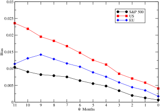
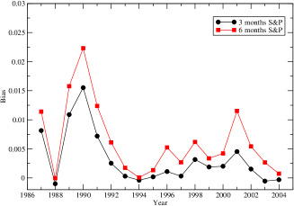
Figure 1: Left: The grand average bias $B(\theta)$ for S&P stocks, US stocks (including S&P stocks) and European stocks, as a function of the time $\theta$ to ead. The statistical error bar is of the order of the size of the symbols. Note that the bias is smallest for S&P stocks, intermediate for EU stocks, and largest for the US stock pool, suggesting a size effect (see Fig. 2). Right: The bias $B(\theta;t)$ for S&P stocks, for $\theta=3$ months and $\theta=6$ months, as a function of the time $t$ (year of the earning announcement). Note that the bias was very small around 1994 and 2003.

The grand average bias $B(\theta)$ is plotted as a function of $\theta$ in Fig. 1 (left), for three different ensemble of stocks: S&P stocks, large pool of US stocks and European stocks. We observe that the bias is positive, in agreement with previous studies, showing that analysts are on average over-optimistic about the result of companies. The bias steadily decreases as $\theta$ decreases; however, expressed in relative terms, the bias on the forecast eps is still on the order of $10\%$ one month before the ead! Fig. 1 (right) shows how on average the bias for a fixed $\theta$ (3 months or 6 months), $B(\theta;t)$ depends on the year of the prediction. One sees that the bias was very strong in the early 90’s, nearly disappeared in 1993-95 to grow again during the Internet bubble, and is back to small values since 2003 (at least for $\theta=3$ months; the bias 6 months ahead is still significant). The reasons for a persistent positive bias in forecasts have been discussed in the past – these can be institutional (e.g.: analysts are paid by institutions that benefit from bullish stock markets), behavioral (e.g: positive recommendations are always easier to publish than negative statements) or affected by positively biased informations released by companies themselves. The decrease of bias is expected because more and more reliable information is available as the ead is approached. If the bias is of institutional/behavioral origin, the decrease is also expected since it becomes more and more untenable to publish knowingly unreliable estimates very shortly before the true number becomes available (similar results can be observed on the UK and JP pools, with biases slightly larger than for the US one).

From the data, we can also study how the average bias depends on the size (market value) of companies. As shown in Fig. 2 (left), there is a clear size effect: the bias is smaller on larger size companies, probably because more people are concerned by the results of these companies; the pressure on analysts to make good forecasts is thus stronger. The size difference might then explain why the bias is larger in EU than for S&P stocks; this explanation is however different from the one proposed in [9] where the difference in bias is attributed to different regulations in the US and in the Eurozone.

We have finally studied how the bias depends on the industry sector in the US. The result is shown in Fig. 2 (see Table I for the sector code), which reveals that there is significant dependence of the bias on the sector. Such a sectorization of errors will be further discussed in Section 5.

Table 1: Economics Sectors
1	Basic Materials
2	Consumer, Cyclical
3	Consumer, Non cyclical
4	Communications
5	Energy
6	Finance
7	Industrial
8	Technology
9	Utilities

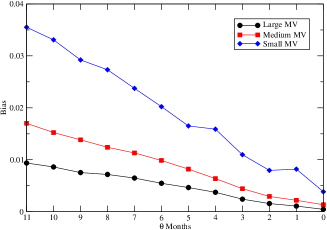
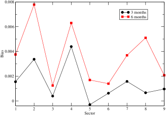
Figure 2: Left: The grand average bias $B(\theta)$ for US stocks, for different market values, as a function of the time $\theta$ to ead. Right: The bias for S&P stocks, for $\theta=3$ months and $\theta=6$ months, as a function of economic sector.

3.3 Forecast errors

We now turn to the forecast error, which measures how far off, typically, the forecast deviates from the actual eps. The result is shown in Figs. 3 and 4, where one sees, respectively, $\Sigma(\theta)$ as a function of $\theta$ and $\Sigma(\theta;t)$ as a function of $t$ for $\theta=3$ months and $\theta=6$ months. One sees that (i) the forecast error, much like the average bias, is larger on the global US pool than on the restricted S&P pool, with the EU pool in-between; (ii) the forecast error weakly decreases with the distance to ead, but the final ($\theta=0$) prediction error is still $100\%$ to $200\%$ of the predicted eps – in other words, the forecast is not only systematically biased, it is also very imprecise; (iii) the forecast error seems to have trended down over the years: it has on averaged decreased by a factor 5 between the late 80’s and nowadays, with a low in the mid-nineties.

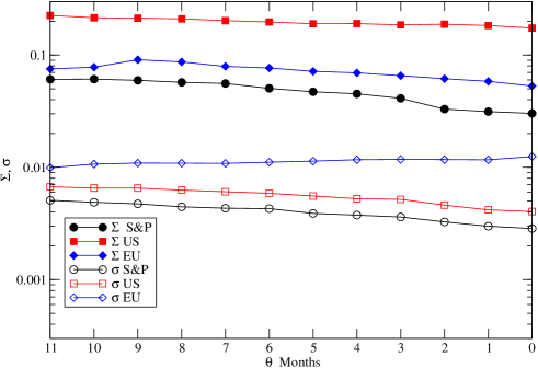
Figure 3: The forecast error $\Sigma(\theta)$ and average dispersion $\sigma(\theta)$ for S&P stocks, US stocks (including S&P stocks) and EU stocks. The forecast error is smallest for S&P stocks and strongest for US stocks. The striking finding is that the forecast dispersion is on average 3-10 times smaller than the forecast error itself!

Point (i) emphasizes the size effect observed in Fig. 2: analysts dealing with larger stocks with a wide investor base produce on average better forecasts than on small caps. Although intuitive, this result is in contradiction with the results of Bagella et al. [9], who report an inverse size effect, but on a smaller sample of US stocks. We have therefore studied the restricted S&P sample and looked for an inverted size effect there but with no success. In fact, small, medium and large caps of the S&P sample have a very comparable forecast error. Hence, we have not been able to reproduce the inverse size effect reported in [9]. The difference might come from the selected pool of stocks, or from the treatment of errors, outliers, etc.

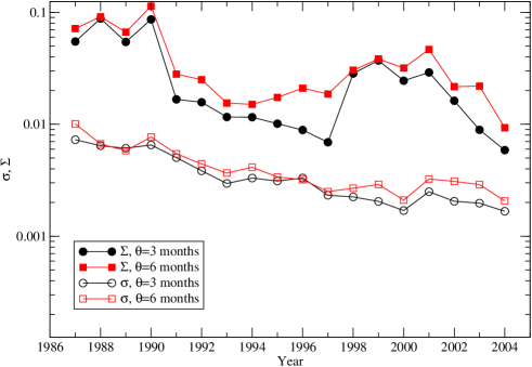
Figure 4: The forecast error $\Sigma(\theta;t)$ and average dispersion $\sigma(\theta;t)$ for S&P stocks, for $\theta=3$ months and $\theta=6$ months, as a function of the time $t$ (year of the earning announcement). Both decrease with years, but the latter is always five to ten times smaller than the former.

It is interesting to compare the performance of analysts forecasts with the simplest ‘no-change’ forecast, which amounts to taking last year’s eps as an estimator of the future eps. When compared with forecasts of similar maturity (i.e. choosing $\theta=11$ months), we find (see Fig. 5) that both fare very similarly in terms of prediction error, but that the no-change forecast is significantly less biased. The situation improves somewhat for analysts as $\theta$ decreases, as of course expected.

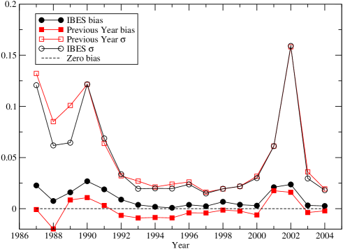
Figure 5: The forecast bias $B(\theta=11;t)$ and forecast error $\Sigma(\theta=11;t)$ compared to the same quantity computed using last year’s eps as a predictor of the future eps.

4 Herding effects

The most striking content of Figs. 3 and 4 is the fact that the forecast dispersion $\sigma$, which measures how much analysts disagree with each other, is much smaller than the forecast error itself (we find the same result for the UK and JP pools). Furthermore, the diversity of opinions decreases with time to ead. These two findings strongly suggest herding effects, as has been discussed and modeled in several previous publications [8, 12]. One could argue that a convergence of prediction is in fact natural because all analysts are perfectly competent and all base their judgment on the same available information, that becomes more precise as the ead is approached. This is however incompatible with the huge amplitude of the ex-post prediction error, which means that the information was in fact quite ambiguous and not sufficient to allow a precise forecast. The rationality scenario would imply that the dispersion is of the same order of magnitude as the prediction error itself, i.e. $\sigma\simeq\Sigma$. The observed inequality $\sigma\ll\Sigma$, on the other hand, can only be explained by a copy-cat mechanism, whereby each analyst progressively biases his forecast toward the average of his fellow analysts, as documented in [8]. The reasons for this strong herding behavior have been discussed in terms of e.g. career motivations (differences between experienced and younger analysts can be observed [11]), or behavioral effects, illustrating Keynes’ observation that it is better to be wrong with the crowd than right against the crowd. In that respect, the improved quality of ‘outlier’ (or bold) forecasts has been noticed in [11].

The above observation suggests to introduce the herding ratio $\phi=\Sigma/\sigma$. From the data of Figs. 3 and 4, we conclude that herding is noticeably stronger in the US, UK and JP ($\phi\approx 10$ for S&P stocks, $\phi\approx 40$ for all US stocks, and $\phi\approx 20$ for JP and UK stocks) than in the EU ($\phi\approx 7$). The reason why EU appears to stand out might be related to the diversity of analysts following European companies. Indeed, we could speculate that analysts from different countries and different backgrounds might be less prone to herding behavior.

While the dispersion of opinions is much smaller than the actual prediction error, it is still interesting to ask if there is some correlation between the lack of agreement between analysts and the difficulty to predict the eps. A scatter plot of the absolute value of prediction error $|b_{\alpha,t-\theta}|$ and the contemporaneous dispersion $\sigma_{\alpha,t-\theta}$ is shown in Fig. 6, together with a linear regression. We find, as expected, a positive intercept (meaning that even in the case of perfect agreement between analysts, they still get the result wrong) and a slope larger than unity. The correlation between the two quantities is found to be $0.46$, meaning that the lack of agreement between analysts still gives some indication of how wrong their prediction is.

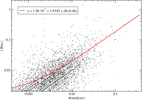
Figure 6: Scatter plot, for all times and all stocks, of the absolute forecast error $|b_{\alpha,t-\theta}|$ versus the contemporaneous dispersion $\sigma_{\alpha,t-\theta}$ for the S&P stocks, and linear regression.

5 Correlation of prediction errors

The above sections were concerned with the variance of the individual forecast errors, which we found to be quite large. However, since we have calculated this as a grand average over all stocks, this large error could be localized in some sectors of activity, or some particular stocks. It is thus interesting to look at the correlation of these forecast errors across different economic sectors. One would a priori expect to see a ‘market mode’ and a sectorization of the forecast errors, much as stock returns. A way to investigate systematically this question is to study the covariance matrix $C_{\alpha,\beta}$ and the correlation matrix $c_{\alpha,\beta}$, defined as:

$$C_{\alpha,\beta}=\langle b_{\alpha,t-\theta}b_{\beta,t-\theta}\rangle_{t,\theta}-\langle b_{\alpha,t-\theta}\rangle_{t,\theta}\langle b_{\beta,t-\theta}\rangle_{t,\theta},$$ (4)

and

$$c_{\alpha,\beta}=\frac{C_{\alpha,\beta}}{\sqrt{C_{\alpha,\alpha}C_{\beta,\beta}}}.$$ (5)

[One could also have chosen not to average over $\theta$ and have $\theta$ dependent correlation matrices]. A way to analyze the content of these matrices is to study their eigenvalues and the corresponding eigenvectors. We expect, much as like the correlation matrix of stock returns, that a large fraction of these eigenvalues is dominated by measurement noise and do not contain useful information, while only the few largest eigenvalues carry meaningful information.

In order to perform this analysis, we have restricted to $M=324$ stocks from the S&P during the period 1990-2003. Using results from Random Matrix Theory [14], we find that only three or four eigenvalues can be distinguished from pure noise. The corresponding eigenvectors are unlocalized, with an inverse participation ratio on the order of $M/2$, meaning that a large fraction of the stocks participate to these correlation modes. Theses eigenvectors corresponding to the largest eigenvalues of $c$ reveal that some sectors dominate, meaning that prediction errors are strong in a some sectors and much weaker in others. Perhaps unexpectedly, the largest eigenvector is not uniform, as one would observe if predictions were over-optimistic or over-pessimistic for the market as a whole. Already at the level of the largest eigenmodes shown on Fig. 7, some sectorization indeed appears as the largest mode is not uniform over the stocks; for example, the errors in sector 3 seem uncorrelated from the rest of the market. Remember that in this sector the bias is also small on average, which is not surprising in view of the relative stability of the demand in this sector (food, drinks, etc). The first mode also shows that large, correlated prediction errors are localized in sectors 2, 4, 6 and 7, while the second mode reveals clearly that sector 6 (Finance) stands out as a special sector, as far as forecast errors are concerned. We have also studied the $\theta$ dependent correlation matrices and found that the inverse participation ratio of the top eigenvectors decrease as the ead is approached, meaning that sectorization of errors increases as $\theta$ decreases. This is again quite expected.

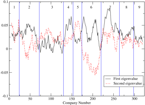
Figure 7: First and second eigenmode of correlation matrix $c$. Note that stocks are ordered by economics sectors. A smoothing of the eigenmode components has been performed for clarity.

6 Additional remarks and conclusion

In this study, we have once more confirmed, on four different, large sets of data, that financial analysts are on average over-optimistic and show a pronounced herding behavior. These effects are however time dependent, and were particularly strong in the early nineties and during the Internet bubble. We have also emphasized that their forecast ability is, in relative terms, quite poor and comparable in quality, a year ahead, to the simplest ‘no change’ forecast. As a result of herding, analysts tend to agree with each other five to ten times more than with the actual result. We have shown that significant differences exist between US stocks and EU stocks, that may partly be explained as a company size effect and not, as conjectured in [9], to differences in regulations and information transparency. Interestingly, herding effects appear to be stronger in the US than in the Eurozone. Finally, we have studied the correlation of errors across stocks and shown that significant sectorization occurs, some sectors being easier to predict than others.

The conclusion is that if the information available to the best experts is so scarce and/or difficult to interpret, resulting in such imprecise and biased estimates of the earnings of companies, one can really wonder what the concept of efficient markets and rational pricing really means. The famous relation between the price of a stock and the sum of expected (discounted) future dividends appears to be nearly empty with such gossamer information. In fact, one can test quantitatively the validity of such a pricing equation. Since dividends are correlated with earnings, a surprise in the announced eps compared to its anticipation should lead to an immediate change of the price of the stock. If earnings per share and dividends per share were equal, a reasonable mean-reverting random walk model for earnings would lead to a perfect correlation between the price change on the ead and the difference between the latest forecast and the actual eps. There are however two complications: (i) dividends per share and eps have a correlation $\rho<1$. For S&P stocks, we find $\rho\approx 0.25$; (ii) on the ead, other news may affect stock prices. A way to estimate their impact is to measure the average increase of volatility on eads compared to normal days. For the same pool of stocks, we find a volatility ratio of $\approx 1.7$. The resulting correlation between stock returns on ead and the unanticipated part of the eps can then easily be computed to be $\approx 0.20$, a factor four larger than the empirical correlation, that we find to be $\approx 0.05$. Such a decoupling between dividends and stock prices is similar to that reported by Shiller in his famous study on excess volatility [3]. One could argue that the measured correlation is small because part of the information is actually already encoded in the price, before the ead, through ‘insider trading’ [15], or through the ‘collective intelligence’ markets are supposed to be endowed with. We have checked that this is not the case by studying the correlation between price changes and eps changes. If the market was correctly anticipating the change of eps, the price change between the day before the previous ead and the day after the last ead should be positively correlated with the change of eps. However, we found empirically a very small, insignificant correlation of $0.02$. So the announced eps should have a much stronger impact on prices, if the classical rational pricing model was correct.

We rather believe that the notion of a true, fundamental price of a company is moot, since nobody, even the best expert, can agree on its value. One can at best estimate a rather broad range, say within a factor of two, of reasonable prices for a given stock [7]. Within this range, prices fluctuate freely – arbitrage cannot be efficient, because of the lack of a reliable estimate of what the true price should be [16]. The volatility is then set by the trading activity itself [17, 18, 19], and can be indeed much larger than what should be expected on the basis of the efficient market theory [3]. Non rational, self-referential and behavioral effects do emerge [20, 21, 16, 22, 23, 24], unleashed by the lack of reliable information, generically unavailable in complex systems – complexity puts de facto strong limits on the very notion of rationality [4, 25, 26]. However, as emphasized in [24], on time scales such that these random fluctuations become of the order of 100 % and reach the boundary of the fuzzy price range alluded to above, one should expect mean reversion effects to become noticeable. For a typical stock with a daily volatility of $3\%$, this corresponds to 1000 days (because $100\approx 3\sqrt{1000}$), or four years. Such a time scale is precisely the typical reversion time scale discovered by De Bondt and Thaler in their paper on overreaction in stock markets [27].

Finally, the strong herding effects between analysts leaves little doubt that similar herding effects exist between investors and market agents at large [20, 21]. This is another nail in the coffin of Efficient Markets. Efficient Markets should reflect the aggregate opinion of incompletely informed, but independent agents, and therefore produce a global, unbiased estimator of the true value of companies. Instead, herding effects can lead to overreactions, bubbles and persistent mispricings, a conclusion of little surprise to the lay-man not acquainted with neo-classical economics.

Acknowledgments: We acknowledge important discussions with J. Kockelkoren, L. Laloux, Y. Lemperiere and M. Potters. We also are grateful to Thomson Financial for providing the data analyzed here.

References

- [1] E. F. Fama, Efficient capital markets: A review of theory and empirical work, Journal of Finance, 25, 383 (1970).
- [2] P. A. Samuelson, Proof that properly anticipated prices fluctuate randomly, Industrial Management Review, 6, 41 (1965).
- [3] R. J. Shiller, Do Stock Prices move too much to be justified by subsequent changes in dividends?, American Economic Review, 71, 421 (1981). R. J. Shiller, Irrational Exuberance, Princeton University Press (2000).
- [4] W. B. Arthur, Complexity in Economic and Financial Markets, Complexity, 1, 1 (1995).
- [5] D. Ruelle, Chance and Chaos, Princeton University Press, 1993.
- [6] P. Bak, How Nature Works: The Science of Self-Organized Criticality, Copernicus, Springer, New York, 1996.
- [7] F. Black, Noise, J. of Finance, 41 529 (1986).
- [8] B. Trueman, Analyst Forecasts and Herding Behavior, Review of Financial Studies, 7, 97-124 (1994).
- [9] M. Bagella, L. Becchetti, R. Ciciretti, The earning forecast bias: a comparative analysis on US and Eurozone stock markets; working paper
- [10] A.M. El-Galfy, W. P. Forbes, An evaluation of US Security Analysts forecasts 1983-1999, working paper.
- [11] H. Hong, J. Kubik, A. Solomon, Security analysts’ career concern and herding or earning forecasts, RAND Journal of Economics, 31, 144 (2000)
- [12] A. Krause, Herding behavior of financial analysts: A model of self-organized criticality, working paper (2003).
- [13] On that point, see J. Sutton, Company growth, the scaling puzzle, Physica A 312, 577 (2002), and refs. therein, and M. Wyart, J.P. Bouchaud, Statistical models for company growth, Physica A 326, 241 (2003) for an alternative point of view.
- [14] L. Laloux, P. Cizeau, J.P. Bouchaud, M. Potters, Noise Dressing of Financial Correlation Matrices, Phys. Rev. Lett. 83, 1467 (1999), see also: J.-P. Bouchaud and M. Potters, Theory of Financial Risks and Derivative Pricing, Cambridge University Press, 2003, chapter 9.
- [15] A. S. Kyle, Continuous auctions and insider trading, Econometrica 53, 1315 (1985).
- [16] A. Shleifer, Inefficient Markets, An Introduction to Behavioral Finance, Oxford University Press (2000).
- [17] T. Odean, Do Investors Trade Too Much?, American Economic Review, 89, 1279 (1999).
- [18] C. Hopman, Are supply and demand driving stock prices?, MIT working paper, Dec. 2002.
- [19] J.P. Bouchaud, Y. Gefen, M. Potters, M. Wyart, Fluctuations and Response in Financial Markets: The subtle nature of ‘random’ price changes, Quantitative Finance 4, 176 (2004).
- [20] A. Kirman, Ants, rationality and recruitement, Quarterly Journal of Economics, 108 137 (1993)
- [21] A. Banerjee, A simple model of herd behaviour, Quarterly Journal of Economics, 107 797 (1992); S. Bikhchandani, D. Hirshleifer, I. Welch, A theory of fads, fashions, custom and cultural changes as infomational cascades, Journal of Political Economy, 100 992 (1992).
- [22] A. Orléan, Le pouvoir de la finance, Odile Jacob, Paris (1999); A quoi servent les marchés financiers ?, in Qu’est-ce que la Culture ?, Odile Jacob, Paris (2001).
- [23] see also: D. Challet, M. Marsili, Y.C. Zhang, The Minority Game, Oxford University Press, 2004.
- [24] M. Wyart, J.P. Bouchaud, Self-referential behaviour, overreaction and conventions in financial markets, e-print cond-mat/0303584, submitted to J. Economic Behaviour & Organisation.
- [25] A. Kirman, Reflections on interactions and markets, Quantitative Finance, 2, 322 (2002).
- [26] On this point, see the discussion in: S. Galluccio, J. P. Bouchaud, M. Potters, Rational decisions, random matrices and spin-glasses, Physica A 259, 449-456 (1998), and J.P. Bouchaud, La (regrettable) complexité des systèmes économiques, Pour La Science, Décembre (2003), p. 142.
- [27] W. de Bondt, R. Thaler, Does the market overreact ?, Journal of Finance, XL, 793 (1985).