Numerical study of a fragile three-dimensional kinetically constrained model

Abstract

We numerically study the three-dimensional generalization of the kinetically constrained East model, the North-or-East-or-Front (NEF) model. We characterize the equilibrium behaviour of the NEF model in detail, measuring the temperature dependence of several quantities: $\alpha$-relaxation time, distributions of relaxation times, dynamic susceptibility, dynamic correlation length, and four-point susceptibility. We show that the NEF model describes quantitatively experimental observations over an exceptionally wide range of timescales. We illustrate this by fitting experimental data obtained both in the mildly supercooled regime by optical Kerr effect, and close to the glass transition by dielectric spectroscopy.

I Introduction

Supercooled liquids can be studied using theoretical models where the density field dynamics is replaced by a coarse-grained mobility field evolving with simple empirical rules based on the idea of dynamic facilitation reviewkcm . Kinetically constrained models (KCM), such as the Fredrickson-Andersen (FA) model fa and the East model east ; Sollich-Evans , have been shown to reproduce well the phenomenology of supercooled liquids. An important feature of these models is that their dynamics becomes spatially correlated harrowell ; garrahan-chandler , i.e., growing timescales are accompanied by growing dynamical lengthscales, giving rise to dynamic heterogeneity as observed in experiments and simulations DHreviews1 ; DHreviews2 ; DHreviews3 ; DHreviews4 .

In this paper, we study by means of extensive numerical simulations the three-dimensional generalization of the East model east , the North-or-East-or-Front (NEF) model NEother . This model is a realization of the ‘arrow’ model of Ref. pnas , but with an externally imposed directional preference while in the arrow model excitations carry an orientation which locally determines the directionality of the dynamics, making the system isotropic pnas . These models were shown to reproduce the dynamic behaviour of a wide range of fragile materials pnas . The present study is complementary to that of Refs. steve1 ; steve2 that considered systems with fully isotropic dynamic facilitation, such as the three-dimensional FA model, which describes strong materials.

The principal aims of this work are the following:

(i) Quantitative characterization of the fragile limit. We report numerical results for a wide range of dynamic observables in the NEF model, describing in detail distributions of the relevant timescales and lengthscales. We also confirm some of the predictions for the arrow model of Ref. pnas .

(ii) Comparison to the strong limit. We contrast our results for the NEF model to those obtained in Refs. steve1 ; steve2 which dealt with the strong limit of isotropic facilitation, such as the three-dimensional FA model.

(iii) Comparison to experimental data. We use the NEF model results to fit experimental data over a wide range of relaxation times, covering both the onset of supercooling, and the regime close to the glass transition.

The paper is organized as follows. We first describe the model and some technical details in Sec. II. We then turn to the study of the relevant timescales, how they are distributed and evolve with temperature in Sec. III. We study spatial aspects of the dynamic in Sec. IV: dynamic heterogeneity and four-point correlations. We compare our numerical results to experimental data in Sec. V, and conclude the paper in Sec. VI.

II Model and simulation details

The NEF model is defined by the Hamiltonian

$$H=\sum_{i=1}^{N}n_{i},$$ (1)

where $n_{i}=0,1$ are $N=L^{3}$ binary variables defined on each site of a cubic lattice of linear size $L$, which has periodic boundary conditions. Physically, $n_{i}=1$ ($n_{i}=0$) describes at a coarse-grained level a site which is mobile (immobile).

The dynamics of the model can be written as follows,

$$n_{i}=0\begin{array}[]{c}\xrightarrow{~{}~{}~{}{\cal C}_{i}~{}c~{}~{}}\\ \xleftarrow[{\cal C}_{i}~{}(1-c)]{}\\ \end{array}n_{i}=1,$$ (2)

where

$$c=\langle n_{i}\rangle=\frac{1}{1+\exp(1/T)},$$ (3)

is the mean concentration of mobile regions and ${\cal C}_{i}$ is the kinetic constraint,

$${\cal C}_{i}=1-\prod_{\langle j,i\rangle^{\prime}}(1-n_{j}).$$ (4)

The prime indicates that the product is restricted to those three sites, $j$, which are north, front, and east nearest neighbours of site $i$. The kinetic constraint (4) implies that site $i$ cannot change state unless at least one of those three neighbours is in the state $n_{j}=1$. The system is therefore more constrained than the corresponding one-spin facilitated FA model, where any of its six neighbours can facilitate the site $i$. In the arrow model, anisotropy is only local and results physically from the empirical observation that facilitation has locally a preferred direction that may persist over a certain length scale even though the system is on average totally isotropic pnas . The NEF model corresponds therefore to having an infinitely large persistence length of dynamic facilitation. This is physically unrealistic, but constitutes a useful limit effectively describing systems with a large but finite persistence of dynamic facilitation footnote .

We performed Monte-Carlo simulations of the NEF model for several temperatures in the range $T\in[0.15,5.0]$, covering over eleven orders of magnitude in relaxation times. Such large time scales can be simulated using a continuous time algorithm Newman-Barkema . As we shall see, this dynamical slow-down is accompanied by the growth of dynamic spatial correlations, and one has to pay attention to possible finite size effects fss . This is however not a serious problem in the present model because even at very large time scales spatial correlations are not very large (see below). At the lowest temperature simulated a system size of $N=32^{3}$ proved to be large enough. Compare this to the system size $N=160^{3}$ used in the strong limit to simulate similar timescales steve2 . Equilibrium behaviour is trivial due to the non-interacting Hamiltonian (1). It is straightforward to produce independent equilibrated initial configurations. Simulations therefore only consist of production runs. Averages are then performed over truly independent initial configurations.

III Time scales

III.1 Global dynamics

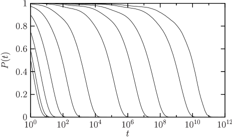
Figure 1: Persistence function, Eq. (5), for temperatures decreasing from left to right: $T=4.0$, 2.0, 1.0, 0.6, 0.4, 0.3, 0.23, 0.2, 0.18, 0.16, and 0.15.

We first consider the spatially averaged dynamics, which may be probed via the mean persistence function,

$$P(t)=\left\langle\frac{1}{N}\sum_{i=1}^{N}P_{i}(t)\right\rangle,$$ (5)

where $P_{i}(t)$ is the single-site persistence function at time $t$, which takes the value $1$ if site $i$ has not flipped up to time $t$, and the value $0$ otherwise. As discussed in Ref. Berthier-et-al , the persistence function $P(t)$ can be seen as the analog of the self-intermediate scattering function, $F_{s}(k,t)$, of a supercooled liquid at wavelengths comparable to the particle diameter footnote2 . Fig. 1 shows, as expected, that the dynamics slows down markedly when temperature is decreased below $T_{o}\approx 1.0$, indicating the onset of slow dynamics in this model pre ; Brumer-Reichman . Physically, $T_{o}$ corresponds to the energy scale of the problem, i.e. the energy needed to create an excitation, see Eq. (3).

The shape of the mean persistence function will be discussed below in some detail. For the moment, we simply note that the long-time decay is non-exponential, as is commonly observed in supercooled liquids. Moreover, the short-time dynamics also presents non-trivial features, see for instance the curve for $T=0.15$ in Fig. 1.

The mean relaxation time, $\tau(T)$, is extracted via the usual relation $P(\tau)=e^{-1}$. In the present context, $\tau$ represents also the $\alpha$-relaxation of the model. The temperature dependence of $\tau$ is shown in Fig. 2. The main observation from this figure is that the mean-relaxation time grows with decreasing temperature in a super-Arrhenius manner, see Fig. 2. The NEF model behaves as a fragile supercooled liquid, as expected pnas . Note however that the ratio $T_{o}/T_{g}\approx 7$ that can be extracted from Fig. 2 is about three times smaller in fragile liquids such as orthoterphenyl.

Various fits are also included in Fig. 2. The high temperature behaviour is well described by a naive mean-field approximation eisinger ; pre ,

$$\tau_{MF}\sim c^{-1}.$$ (6)

This behaviour breaks down below $T_{o}$, where dynamics is dominated by local fluctuations of the mobility. Generalizing to three dimensions the results for the East model east ; Aldous-Diaconis ; pnas , we expect that in the limit of small temperature, the time scale behaves as

$$\tau\sim c^{-\Delta(T)},$$ (7)

with $\Delta(T)\approx b/T$ at low $T$, where $b$ is a constant. Since $c\sim e^{-1/T}$, Eq. (7) implies an exponential inverse temperature squared dependence at low temperatures, $\tau\sim e^{b/T^{2}}$. In fact, an empirical fit using

$$\Delta(T)=a+\frac{b}{T},$$ (8)

allows one to describe the whole temperature range studied, using $b=0.634$ and $a=1.1$. The supposedly exact low-temperature result, $\Delta(T)=(3\ln 2T)^{-1}$, works well for very large relaxation times. Indeed we find that a plot of $T^{2}\log\tau$ vs. $1/T$ nicely converges to the theoretical value $(3\ln 2)^{-1}$ (not shown). At low temperatures, the $\alpha$-relaxation in the NEF model therefore follows a Bässler law bassler .

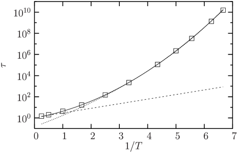
Figure 2: Points: Mean relaxation time from $P(\tau)=e^{-1}$. The lines represent various fits. Dashed line is the high-temperature Arrhenius behaviour, $\tau\sim\exp(1/T)$. Full line is $\tau(T)\sim\exp(\Delta(T)/T)$ with $\Delta(T)=0.634/T+1.1$. The dotted line shows that a Vogel-Fulcher form, $\tau\sim\exp[2.3/(T-0.06)]$, fits the low temperature data with an unphysical finite $T$ singularity.

Fig. 2 also shows that the low $T$ data can be fit using the Vogel-Fulcher law, $\tau_{VF}\sim\exp\left[A/(T-T_{0})\right]$. The Bässler and Vogel-Fulcher curves are hardly distinguishable for over eight orders of magnitude, as has been observed before when fitting experimental data bassler . In our case, it is evident that the finite temperature singularity of the Vogel-Fulcher law is completely unphysical.

As will be discussed below, the fragile behaviour of the NEF model results from the existence of a hierarchy of lengthscales governing the dynamical behaviour. It is therefore not surprising that the relaxation time in this model does not follow the Adam-Gibbs relation which is argued to link dynamics and thermodynamics of supercooled liquids ag ; angell . For the NEF model, the entropy has essentially an Arrhenius behaviour at low temperatures. The Adam-Gibbs relation thus predicts the relaxation time to grow as a double exponential of the inverse temperature. This vastly overestimates the growth of $\tau$, which follows the Bässler law, Eqs. (7,8). In the same vein, naively extracting a Kauzmann temperature by linearly extrapolating the entropy to zero in the same temperature range where the Vogel-Fulcher law seems to apply (see Fig. 2), gives a value $T_{K}\approx 0.16$, which is very different from the Vogel-Fulcher temperature $T_{0}\approx 0.06$ found above. Although $T_{0}$ and $T_{K}$ are ill-defined temperatures in our case, experimentally they are often found to be close in fragile liquids, a feature which is not quantitatively reproduced by the NEF model.

III.2 Distribution of relaxation times

The mean relaxation time $\tau(T)$ captures only in part the relaxation behaviour of the model. We consider in this subsection the distribution of relaxation times, $\pi(t)$, related to the mean persistence function via pre

$$P(t)=\int_{t}^{\infty}dt^{\prime}\pi(t^{\prime}).$$ (9)

These distributions are shown in Fig. 3.

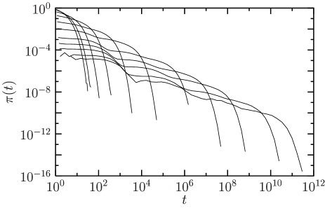
Figure 3: Distribution of persistence time $\pi(t)$, see Eq. (9), for temperatures as in Fig. 1, decreasing from left to right.

As mentioned above, the long-time tail of the persistence function is well-described by a stretched exponential form, which implies the following long-time behaviour for the distribution of relaxation times,

$$\pi(t)\sim\frac{t^{\beta-1}}{\tau^{\beta}}\exp\left[-\left(\frac{t}{\tau}\right)^{\beta}\right],$$ (10)

valid for when $t\gg\tau$. As for the East model Sollich-Evans ; Buhot ; jcp , we find that the stretching exponent $\beta$ decreases with $T$ in the regime $T<T_{o}$, from its high temperature value $\beta=1$.

As can be guessed from Figs. 1 and 3, using $\tau(T)$ and $\beta(T)$ as unique fitting parameters does not allow for a satisfactory description of the whole decay of the persistence function and distribution of relaxation times. This becomes evident when data are presented in an alternative way. Following the experimental literature, we show the data obtained from the distribution of time scales in a frequency representation via bloch

$$\chi^{\prime\prime}(\omega)={\rm Im}~{}\int_{-\infty}^{\infty}\pi(\log(\tau))\frac{1}{1+i\omega\tau}\,d\log\tau,$$ (11)

as is often done with dielectric susceptibility measurements. This will also allow us to make quantitative comparisons to experiments below. The results for $\chi^{\prime\prime}(\omega)$ are displayed in Fig. 4. At temperature $T=0.18$ we show on top of the data the Fourier transform of the stretched exponential fit to the long time tail of $P(t)$. The fit is clearly incorrect in this representation, although it would look acceptable in most of a plot such as in Fig. 1. In fact, deviations appear when $\omega\tau>1$, corresponding to $t<\tau$ in the time domain. This reveals the presence of ‘additional processes’ on the ‘high-frequency flank’ of the $\alpha$-relaxation.

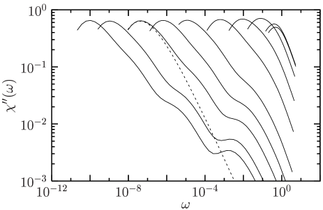
Figure 4: Imaginary part of the dynamic susceptibility defined in Eq. (11), for temperatures as in Fig. 1, decreasing from right to left. For $T=0.18$, we also show as a dashed line the Fourier transform of the stretched exponential fit to the long time tail of the persistence function, revealing ‘additional processes’ on the ‘high-frequency flank’ of the $\alpha$-relaxation.

This feature is obviously reminiscent of the ‘high-frequency’, or ‘Nagel’ wing extensively studied by dielectric spectroscopy in several materials nagel . The wing is usually observed in fragile glass-formers, but its precise nature has not been fully elucidated. Despite initial claims of certain universal behaviour of the high-frequency wing, more recent investigations seem to favour the interpretation that the phenomenon does not obey universal scaling nagel . This is compounded by the observation that the amplitude of the phenomenon also seems to depend on the technique used to study it rossler-epjb .

In our case, the physical interpretation of the wing is very clear. The relaxation of the NEF model proceeds in a hierarchical manner, just as in the one-dimensional case garrahan-chandler ; Sollich-Evans . In order to relax a domain of immobile regions of size $\ell$, a region of size $\ell/2$ must first be relaxed, which itself necessitates the relaxation of a domain of size $\ell/4$, etc., down to the smallest size $\ell=1$. This implies an energy cost $\Delta E(\ell)\sim\ln\ell$, from which the Bässler form, Eq.(8), and stretched exponential decay, Eq. (10), follow garrahan-chandler . Interestingly, the hierarchy also shows up in the distributions of Figs. 3 and 4 at time scales shorter than the $\alpha$-relaxation in a manner reminiscent of the experimental finding of additional short-time processes. Due to the underlying lattice structure of the model, the hierarchy is discrete rather than continuous, as can be indeed observed in Fig. 4. Notice also that there is no ‘fast’ process at the microscopic time scale, $\omega\sim 1$, in our system. This is a consequence of coarse-graining by which molecular vibrations are removed.

These results show that the pattern of dynamical relaxation of the NEF model is quantitatively accurate on a wide frequency range. This will be shown explicitly in Sec. V where dielectric susceptibility data taken close to the experimental glass transition are compared to the NEF model results. We recall that in the strong case the large-time decay was found to be purely exponential, while short-time processes had a much smaller magnitude steve2 . This prediction is however hard to confirm experimentally since strong liquids are not easy to study by dielectric spectroscopy leheny .

Physically, our results also suggest that the high-frequency wing observed in fragile glass-formers is an intrinsic feature of the $\alpha$-relaxation linked in a direct way to their dynamical hierarchical structure which is also at the origin of stretched relaxation and fragile behaviour.

When the relaxation time is moderate, an even more complex behaviour is observed due to the influence of clusters of defects. Such dynamic objects are irrelevant at low temperatures, but can influence the short-time dynamics just below $T_{o}$, as discussed in detail in Ref. pre . These clusters were in particular shown to be responsible for the temperature behaviour of a number of quantities discussed in some numerical works. Clusters also produce additional short-time processes visible in the distributions $\pi(t)$ when temperature is not too low pre . Interestingly in the present context, these patterns closely resemble the ones observed experimentally in mildly supercooled liquids and usually explained in terms of mode-coupling theory mct . This will be demonstrated in Sec. V, where data recently fitted via mode-coupling theory sperl are also fitted using the NEF model.

IV Length scales

IV.1 Dynamic heterogeneity

The growth of timescales in the NEF model is accompanied by growing spatial correlations as the system approaches its critical point at $T=0$. These correlations are purely dynamical in origin, and give rise to dynamic heterogeneity garrahan-chandler ; Berthier-et-al . Figures 5 and 6 serve to illustrate this phenomenon, as we now explain.

We quantify the local dynamics via the local persistence function $P_{i}(t)$. For a given temperature we run the dynamics for a time $t^{\star}$, such that $P(t^{\star})=1/2$, meaning that half of the sites have flipped at least once. We colour white persistent (immobile) spins, for which $P_{i}(t^{\star})=1$, and black transient (currently or previously mobile) spins, for which $P_{i}(t^{\star})=0$. Figure 5 shows the local persistence function for the NEF model at two different temperatures, $T_{o}=1.0$ and $T=0.15\ll T_{o}$. Clearly, the low-temperature dynamics is spatially heterogeneous, and the spatial correlations of the local dynamics grow as $T$ is decreased. The ‘critical’ nature of dynamic clusters is apparent: the pictures are reminiscent of the spatial fluctuations of an order parameter close to a continuous phase transition, such as the magnetization of an Ising model near criticality. In our case, the order parameter is a dynamic object, the persistence function, and the critical fluctuations are purely dynamical in origin fss .

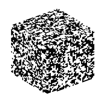
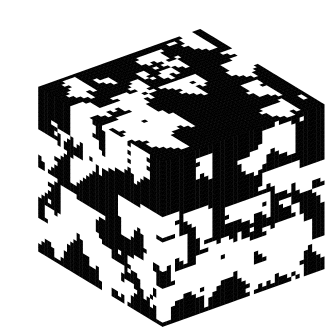
Figure 5: Spatial distribution of the local persistence at time $t^{\star}$ such that $P(t^{\star})=1/2$ (i.e., 50% of sites, shown in black, have flipped by time $t^{\star}$) at temperatures $T=1.0$ (top) and $T=0.15$ (bottom) for a system size $L=40$ in both cases. The appearance of dynamic critical fluctuations when $T\to 0$ is evident.

It is interesting to note that these figures are qualitatively different from the ones obtained in the strong case where dynamic facilitation is isotropic. One can clearly distinguish in Fig. 5 the North, East and Front directions of facilitation, implying that wandering of excitations in the other three directions is forbidden. Domains of Fig. 5 appear much less rough than the ones obtained in the isotropic case steve2 . In that sense, increasing the fragility is similar to increasing the ‘surface tension’ of the dynamic domains observed in Fig. 5. The same observation applies to an even more fragile system, the two-spin facilitated FA model in two dimensions, where the corresponding domains resemble a polydisperse assembly of squares harrowell .

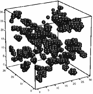
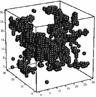
Figure 6: Visualization of 5% of the sites that relax faster (top) and slower (bottom) in a given run at $T=0.18$ for a system size $L=30$. Fast/slow sites are painted as spheres to highlight the similarity between heterogeneity in lattice models to that in atomistic models. The fast clusters in the top figure are less compact than the slow ones in the bottom figure as a consequence of relaxation via point like excitations. See the text for details.

The qualitative observations of dynamic heterogeneity performed in numerical or experimental works can also be made in the present coarse-grained model. We show in Fig. 6 the analog of spatial clustering of subsets of fast and slow sites. To build these snapshots, we represent a given percentage, 5%, of the sites that relax faster or slower, i.e. we show those sites for which the persistence time is among the 5% smaller or larger in a randomly chosen run at temperature $T=0.18$.

One observes that the fastest sites are not randomly located in space, but clustered in ‘non-compact’ or ‘stringy’ objects, similar to those observed in simulations and experiments string ; harrowell2 ; weeks . The shape of these objects is a consequence of the existence of point defects of mobility. When a defect moves, it induces those sites along its trajectory to relax, so leaving in its wake a string of fast sites.

In Fig. 6 we also show 5% of the sites which are slowest, using the same simulation temperature as before. A more compact structure is seen. This is again the consequence of the relaxation via point defects of mobility. The slowest sites belong to regions of space devoid of defects which take then a very long time to be visited by defects. These large domains are thus slowly relaxed. It is the bulk of these slow domains that is observed in Fig. 6. Note finally that at large times, the distribution of slow cluster sizes seems very wide, since some isolated sites which have been not been visited by defects coexist with the very large domains discussed above.

Since our comments on Fig. 6 are mainly qualitative, it should come as no surprise that snapshots built in this fashion in the isotropic case are very similar steve2 .

Finally, it is interesting to compare these figures to those in previous publications garrahan-chandler ; pre , in which space-time diagrams of one dimensional kinetically constrained models were presented. There, spatio-temporal ‘bubbles’ of immobile regions, bounded by diffusing point defects were presented. In the present model these bubbles become $(3+1)$-dimensional objects, and Fig. 6 their three-dimensional spatial projections of trajectories of various time extensions.

IV.2 Spatial correlations

We now quantify these qualitative observations via appropriate statistical correlators. We measure spatial correlations of the local dynamics via the following spatial correlator of the local persistence function,

$$C(r,t,T)=\frac{1}{Nf(t)}\sum_{i=1}^{N}\Big{[}\langle P_{i}(t)P_{i+r}(t)\rangle-P^{2}(t)\Big{]},$$ (12)

where the function $f(t)=P(t)-P^{2}(t)$ in the denominator ensures the normalization $C(r=0,t,T)=1$. Alternatively, one can take the Fourier transform of (12), giving the corresponding structure factor of the dynamic heterogeneity,

$$S(q,t,T)=\frac{1}{Nf(t)}\sum_{k,l=1}^{N}\Big{[}\langle P_{k}(t)P_{l}(t)\rangle-P^{2}(t)\Big{]}e^{iq(k-l)},$$

for wavevectors defined in the first Brillouin zone of the cubic lattice.

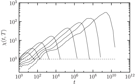
Figure 7: Dynamic ‘four-point’ susceptibility, Eq. (13), at temperatures $T=1.0$, 0.6, 0.4, 0.3, 0.23, 0.2, 0.18, and 0.16 (from left to right).

Finally, the zero wavevector limit of $S(q,t,T)$ defines a dynamic ‘four-point’ susceptibility, $\chi(t,T)=S(q=0,t,T)$, which can be rewritten as the normalized variance of the (unaveraged) persistence function, $p(t)\equiv N^{-1}\sum_{i=1}^{N}P_{i}(t)$,

$$\chi(t,T)=\frac{N}{f(t)}\big{[}\langle p^{2}(t)\rangle-\langle p(t)\rangle^{2}\big{]}.$$ (13)

It should be noted that normalizations also ensure that $\chi(t,T)$ remains finite in the thermodynamic limit, except at a dynamic critical point such as the ones discussed in Refs. steve1 ; mct2 .

Figure 7 shows the time dependence of the susceptibility (13) for various temperatures. The behaviour of $\chi$ is similar to that observed in atomistic simulations of supercooled liquids DHreviews3 . The susceptibility develops at low temperature a peak whose amplitude increases, and whose position shifts to larger times as $T$ decreases. As expected, the location of the peak scales with the relaxation time $\tau(T)$, indicating that dynamical trajectories are maximally heterogeneous when $t\approx\tau(T)$.

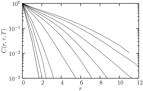
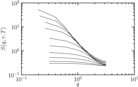
Figure 8: Top: Spatial correlator of dynamic heterogeneity at the relaxation time $\tau(T)$. Temperatures as in Fig. 7 decrease from left to right. Bottom: corresponding structure factor. Temperatures as in Fig. 7 decrease from bottom to top.

In Figure 8 we show the correlator $C(r,t,T)$ and the structure factor $S(q,t,T)$ for different temperatures and fixed times $t=\tau(T)$ where dynamic heterogeneity is maximal. These correlation functions confirm, as suggested by Fig. 5, that a dynamic length scale associated with spatial correlations of mobility develops and grows as $T$ decreases: spatial correlations decay more slowly with distance as $T$ decreases, while a peak in the structure develops and grows at $q=0$.

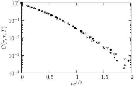
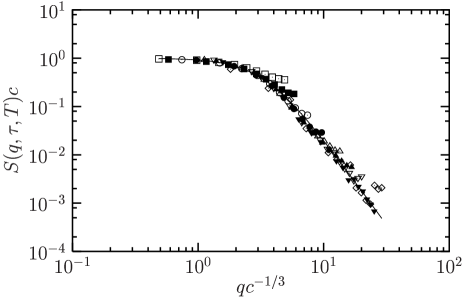
Figure 9: Top: Spatial correlator rescaled with the form $C(r)\sim{\cal C}(r/\xi)$, $\xi\sim c^{-1/3}$. Bottom: Rescaled structure factor with $\chi=S(q=0)\sim c^{-1}$ and $\xi\sim c^{-1/3}$. Full line interpolates between $S(q\to 0)\sim const$ and $S(q\to\infty)\sim k^{-3.58}$.

It is possible to extract numerically the value of the corresponding dynamic length scale, $\xi(T)$, at each temperature. To do so, we study in detail the shape of the correlation functions shown in Fig. 8. As for standard critical phenomena, we find that the dynamic structure factor can be rescaled according to

$$S(q,\tau,T)\sim\chi(\tau,T)\,{\cal S}\left(q\xi\right),$$ (14)

where the scaling function ${\cal S}(x)$ has the following asymptotic behaviours in the scaling regime, $\xi\gg 1$:

$${\cal S}(x\to 0)\sim const,$$ (15)

$${\cal S}(x\to\infty)\sim x^{2-\eta}.$$ (16)

Both the susceptibility $\chi$ and the dynamic length scale $\xi$ estimated at time $t=\tau$ behave as power laws of the defect concentration,

$$\chi\sim c^{-\gamma},\quad\quad\xi\sim c^{-\nu}.$$ (17)

These relations imply that the exponents $\gamma$ and $\nu$ should be numerically accessible by adjusting their values so that a plot of $c^{\gamma}S$ versus $qc^{-\nu}$ is independent of temperature. We show such a plot in Fig. 9, and we find that the values $\gamma\approx 1$ and $\nu\approx 1/3$ lead to a good collapse of the data. The exponent $\gamma$ can be independently and more directly estimated from Fig. 7 by measuring the height of the maximum of the susceptibility for various concentrations. The result is also well fitted to the power law $c^{\gamma}$ with $\gamma\approx 1$. We find also that the scaling function $S(x)$ is well-described by an empirical form $S(x)=1/(1+x^{2-\eta})$, consistent with Eq. (16). Thus we can determine the value of the ‘anomalous’ exponent, $\eta$. We find that the theoretically expected $\eta=-\ln 3/\ln 2\approx-1.58$ describes the data very well garrahan-chandler . The fact that this exponent is much more negative than in the strong case of the FA model quantifies our observation that domains of Fig. 5 were much less rough in the NEF model than in the FA model, i.e., that dynamic domains of fragile systems have smoother boundaries than those of strong ones.

The spatial correlator $C(r,\tau,T)$ also obeys scale invariance, and we find that

$$C(r,\tau,T)\sim{\cal C}\left(\frac{r}{\xi},\tau\right),$$ (18)

with the asymptotic behaviour ${\cal C}(x\to 0)\sim x^{-0.58}$, as a result of a generalized Porod’s law. The scaling behaviour (18) is presented in Fig. 9, which also confirms the temperature dependence of the correlation length, $\xi\sim c^{-1/3}$ pnas . It is interesting to note that the relation between susceptibility and length is very different in the strong and fragile cases, since we find that $\chi\sim\xi^{3}$ in the NEF model, while the scaling is closer to $\chi\sim\xi^{2}$ in the FA case steve2 .

V Comparison to experimental data

In this section, we use the numerical results obtained in previous sections to fit experimental data with the NEF model. In doing so there are several points that need to be considered.

First, the model we use is meant to be a description of supercooled liquids which is coarse-grained both in time and space, and lives on a lattice. We are thus dealing with discrete, rather than continuous, spatial degrees of freedom, and the very short-time dynamics of the liquid is removed. By construction, this produces discrepancies between real data on liquids and numerical NEF model data, especially for short times and small lengths. This is a small price to pay in such an approach given the large number of features that can still be satisfactorily accounted for with the NEF model.

Second, we have some freedom on how to relate real experimental timescales and Monte Carlo steps in the simulation. This will be done empirically, and we find that the expected equivalence, 1 MC step $\approx$ few ps pnas , works well, independently of the temperature. Explicitly, we found that 1 MC $\in[1,10]$ ps for the whole range of experimental data we have considered nagel ; fayer .

Third, one must adjust the temperature given in Kelvin in experiments to the adimensional $T$ of the simulations. This amounts to fitting the value of an energy scale, $J$, which should appear on dimensional grounds in front of the Hamiltonian (1). In principle, $J$ could be fixed independently by fitting, say, viscosity data of a given liquid before using the corresponding temperatures to fit more detailed dynamic data in what would be a zero-parameter fitting procedure. We have done the correspondence in a less constrained manner, adjusting $T$ in the simulation to give a good fit to the data. Very satisfactorily, though, we end up with a correspondence between numerical and experimental temperatures which is well described by linear relations, as it should be at low temperatures pnas .

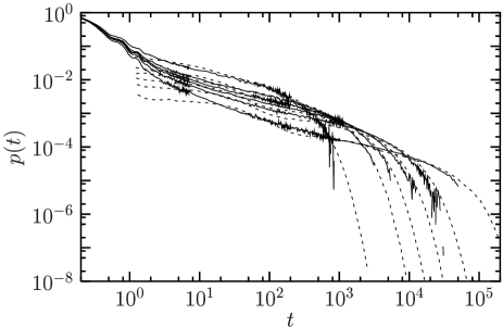
Figure 10: Optical Kerr Effect experimental for supercooled liquid 2-biphenylmethanol (full lines from Ref. fayer ) at temperatures $T=359$ K, 327 K, 319 K, 311 K, 303 K, 291 K (from left to right). Dashed lines are corresponding data for the NEF model at temperatures $T=0.4$, 0.34, 0.32, 0.3, 0.28 and 0.25 (from left to right). Time is counted in picoseconds in the experiments, in Monte Carlo steps in simulations.

In Fig. 10, we show the result of this fitting procedure as applied to recent data measured using the so-called optical Kerr effect oke ; fayer . This technique has several advantages. It extends for over five orders of magnitude in time. The quantity measured is the derivative of a time correlation function, and therefore the analog of the distribution of time scales, $\pi(t)$, discussed above. And vibrations, which are neglected in our approach, affect very little the measured decay in the timescales of interest.

In Ref. fayer , the experimental results were fitted using the empirical form

$$\pi(t)=[pt^{-1+C}+dt^{b-1}]\exp(-t/\tau),$$ (19)

with the values $b\approx 0.8-0.85$ and $C\approx 0.-0.2$ consistently found in different liquids. The $1/t$ behaviour of $\pi(t)$ obtained at short times when $C=0$ implies a $\log{t}$ behaviour of the time correlator. This was taken as a challenging result to mode-coupling theory which does not naturally predict such patterns, as can be seen when asymptotic analytic results are considered mct . These data were however recently virtually perfectly fitted using a standard schematic version of the mode-coupling theory, therefore nullifying the criticisms raised in the experimental work sperl . Note that several fitting parameters are allowed by the mode-coupling fits, which are performed using a two-correlator schematic model: coupling constant, distance to the dynamic singularity and various numerical factors adapting theoretical time scales to the experimental ones. By contrast, we make use of just one free parameter in Fig. 10.

The ‘nearly logarithmic decay’ of correlations has a simple explanation in our approach. At modest temperatures, $T\lesssim T_{o}$, there is a coexistence of isolated excitations, responsible for ‘slow processes’, and rapidly relaxing clusters of excitations; see Ref. pre for a detailed discussion of the related temperature crossovers. This coexistence manifests as a nearly flat distribution $\pi(\log t)$ over a wide range of timescales. This translates into a $1/t$ behaviour of $\pi(t)$, and logarithmic decay of $P(t)$, as observed in Fig. 10. This explanation, moreover, predicts that the effective exponent $C$ appearing in Eq. (19) should acquire a slight temperature dependence, and change from $C<0$, when fast processes dominate closer to $T_{o}$, to $C>0$ at lower temperature when slow processes become dominant. This is precisely what is found in experiments fayer . This subtlety is also accounted for by mode-coupling theory sperl .

The only real discrepancy between fits and data is visible at very short time, as was anticipated, but the overall quantitative agreement is very good. As already suggested by the qualitative analysis of Ref. pre , our theoretical approach can be used even far above the experimental glass transition. Mode-coupling theory is thought to be applicable in this regime, under the assumption that the dynamics at modest supercooling is different from that near $T_{g}$. As in Ref. pre , our results here suggest that this may not be the case.

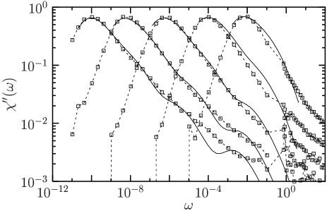
Figure 11: Dielectric susceptibility data for Salol obtained from the authors of Refs. viot at temperatures $T=255K$, $243K$, $233K$, $225K$, and $219K$ (from right to left). Full lines are corresponding data for the NEF model at temperatures $T=0.385$, $0.26$, $0.198$, $0.168$, and $0.15$ (from left to right). Time is counted in units of 10 ps in the experiments, and in Monte Carlo units in the simulations.

One of the advantages of the present approach on mode-coupling theory is that it does not produce an unphysical singularity at a temperature above $T_{g}$, and it can therefore be used down to very low temperatures and large relaxation times. In Fig. 11 we use the NEF model to fit dielectric data taken on Salol nagel . As before, the fits are done using a single free parameter. Fig. 11 shows that the overall agreement is again very good. Note in particular that the high-frequency wing is correctly accounted for by the (discrete) hierarchy of dynamic lengthscales discussed in the previous sections.

Again, discrepancies due to coarse-graining are evident: absence of short-time processes, and discreteness of the hierarchy of time scales. Discrete scales are particularly evident in the Nagel wing, where numerical data only produce the ‘skeleton’ of the wing instead of a smooth curve. Note that the same experimental data were fitted in Ref. viot using a frustration limited domain scaling picture of the glass transition: seven fitting parameters were used there to obtain a satisfactory fit. Such data are usually fitted in experimental papers by empirical forms involving again several free parameters bloch .

Consider, finally, the scaling of lengths and times. Figure 12 shows dynamic scaling in three different model systems: the three-dimensional FA model (indicated as ‘strong’; data from Refs. steve2 ), the present NEF model data (indicated as ‘fragile’), and the Kob-Andersen Lennard-Jones binary mixture ka (‘LJ’ in the figure; data from Ref. steve1 ). The figure shows that in the fragile case the growth of dynamic lengthscales is much less pronounced than in the strong one. This is one of the central predictions of the dynamic facilitation approach pnas . It is a consequence of the temperature dependent dynamic exponent of East-like models such as the NEF model, in contrast to strong systems where dynamic lengths go as a fixed power of the relaxation time. Note that a figure qualitatively similar to Fig. 12 would be obtained for the four-point susceptibility as a function of relaxation time.

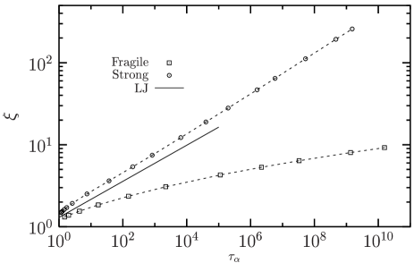
Figure 12: Dynamic scaling of timescales versus lengthscales in the strong three-dimensional FA model steve1 , the fragile three-dimensional NEF model, and three-dimensional binary Lennard-Jones mixture steve1 .

This slow growth of lengthscales in the NEF model is also compatible with the modest size of heterogeneities as suggested by experiments near $T_{g}$ DHreviews2 . Interestingly, the LJ mixture appears in this representation as a fairly strong system, despite the common assumption that it is a good model for fragile liquids. The theoretical and numerical findings reported in Fig. 12 offer a solution to the paradox that experimentally measured length scales are very small when compared to extrapolations performed from numerical works DHreviews2 ; DHreviews3 .

VI Conclusions

In summary, we have presented an extensive numerical study of the North-or-East-or-Front model, the three-dimensional generalization of the East facilitated spin model. The NEF model, whose dynamical rules have an externally imposed asymmetry, is in the same universality class of the more physical arrow model of Ref. pnas in the limit of maximal directional persistence, and therefore models the behaviour of fragile, super-Arrhenius, glass formers.

We have characterized the equilibrium dynamics of the NEF model through measurements of the $\alpha$-relaxation timescales, distributions of relaxation times, and the growth of dynamic correlation lengths and four-point susceptibilities. We find that $\tau_{\alpha}$ follows a Bässler law of exponential-inverse-squared temperature dependence, and that the dynamic correlation length grows as $\xi\sim c^{-\nu}$ with $\nu\approx 1/3$, where $c$ is the equilibrium concentration of excitations, while the dynamic susceptibility grows as $\chi\sim c^{-\gamma}$ with $\gamma\approx 1$. These results confirm some of the expectations of Ref. pnas for the arrow model, in particular the quasi one-dimensional nature of the dynamics in all dimensions. The decay of the four-point structure factor, $S(k)\approx k^{-2-1.58}$, is a direct generalization of the result for the 1D East model garrahan-chandler , and an indication of hierarchical dynamics in the NEF model. These two features, persistence of directionality and hierarchical dynamics, give rise to fragile behaviour pnas .

We have shown how the NEF model can be used to rationalize experimental observations over a wide range of temperatures and timescales. We have fitted correlation data in the time domain, obtained in the mildly supercooled regime by optical Kerr effect fayer , with the NEF model predictions. This provides an interpretation of the quasi logarithmic time dependence of correlations based on the coexistence of isolated excitations and clusters of excitations, which occurs when the system is crossing over from a regime of homogeneous dynamics at high $T$ to one of heterogeneous dynamics at low $T$ pre . We have shown how the NEF model can also be used to describe dielectric susceptibility data, in the frequency representation, measured close to the glass transition by dielectric spectroscopy. Interestingly, the NEF model successfully accounts for the excess high-frequency or Nagel wing nagel .

The results presented in this paper add to the list pnas ; jcp ; jung ; Berthier-et-al of phenomenological observations that can be quantitatively understood within the dynamic facilitation approach.

- (1) F. Ritort and P. Sollich, Adv. in Phys. 52, 219 (2003).
- (2) G.H. Fredrickson and H.C. Andersen, Phys. Rev. Lett. 53, 1244 (1984); J. Chem. Phys. 83, 5822 (1985).
- (3) J. Jäckle and S. Eisinger, Z. Phys. B 84, 115 (1991).
- (4) P. Sollich and M.R. Evans, Phys. Rev. Lett. 83, 3238 (1999).
- (5) P. Harrowell, Phys. Rev. E 48, 4359 (1993).
- (6) J.P. Garrahan and D. Chandler, Phys. Rev. Lett. 89, 035704 (2002).
- (7) H. Sillescu, J. Non-Cryst. Solids 243, 81 (1999).
- (8) M.D. Ediger, Annu. Rev. Phys. Chem. 51, 99 (2000).
- (9) S.C. Glotzer, J. Non-Cryst. Solids, 274, 342 (2000).
- (10) R. Richert, J. Phys: Condens. Matter 14, R703 (2002).
- (11) Other generalizations of the East model include the North-and-East model, where a site can only change its state if two of its neighbours, for example to the east and north, are simultaneously in their excited state; see J. Reiter, F. Mauch and J. Jackle, Physica A 184, 493 (1992).
- (12) J.P. Garrahan and D. Chandler, Proc. Natl. Acad. Sci. USA 100, 9710 (2003).
- (13) S. Whitelam, L. Berthier, and J.P. Garrahan, Phys. Rev. Lett. 92, 185705 (2004).
- (14) S. Whitelam, L. Berthier, and J.P. Garrahan, cond-mat/0408694.
- (15) Beyond the one-spin facilitated FA model, Fredrickson and Andersen have also introduced more constrained models, namely -spin isotropically facilitated models with . These models do exhibit fragile behaviour fa , but they are in a sense not realistic since they are characterized by exponentially diverging activation energies giulio , a feature not observed in real liquids.
- (16) C. Toninelli, G. Biroli, and D.S. Fisher, Phys. Rev. Lett. 92, 185504 (2004).
- (17) M.E.J. Newman and G.T. Barkema, Monte Carlo Methods in Statistical Physics (Oxford University Press, Oxford, 1999).
- (18) L. Berthier, Phys. Rev. Lett. 91, 055701 (2003).
- (19) L. Berthier, D. Chandler, and J.P. Garrahan, cond-mat/0409428.
- (20) For a detailed study of correlation in the East model, especially the behaviour of the persistence at very long times (beyond the alpha-relaxation time regime of interest to us here) see P. Sollich and M.R. Evans, Phys. Rev. E 68, 031504 (2003).
- (21) L. Berthier and J.P. Garrahan Phys. Rev. E 68, 041201 (2003).
- (22) Y. Brumer and D.R. Reichman, Phys. Rev. E 69, 041202 (2004).
- (23) S. Eisinger and J. Jackle, J. Stat. Phys. 73, 643 (1993).
- (24) D. Aldous and P. Diaconis, J. Stat. Phys. 107, 945 (2002).
- (25) H. Bässler, Phys. Rev. Lett. 58, 767 (1987).
- (26) G. Adams and J.H. Gibbs, J. Chem. Phys. 43, 139 (1958).
- (27) R. Richert and A. Angell, J. Chem. Phys. 108, 9016 (1998).
- (28) A. Buhot and J.P. Garrahan, Phys. Rev. E 64, 21505 (2001).
- (29) L. Berthier and J.P. Garrahan J. Chem. Phys. 119, 4367 (2003).
- (30) T. Blochowicz, C. Tschirwitz, S. Benkhof, and E.A. Rössler, J. Chem. Phys. 118, 7544 (2003).
- (31) P.K. Dixon, L. Wu, S.R. Nagel, B.D. Williams, and J.P. Carini, Phys. Rev. Lett. 65, 1108 (1990); U. Schneider, R. Brand, P. Lunkenheimer, and A. Loidl, Phys. Rev. Lett. 84, 5560 (2000).
- (32) A. Brodin, R. Bergman, J. Mattsson, and E.A. Rössler, Eur. Phys. J. B 36, 349 (2003).
- (33) R.L. Leheny, Phys. Rev. B 57, 10537 (1998).
- (34) W. Götze, J. Phys.: Condens. Matter 11, A1 (1999).
- (35) W. Götze and M. Sperl, Phys. Rev. Lett. 92, 105701 (2004).
- (36) C. Donati, J.F. Douglas, W. Kob, S.J. Plimpton, P.H. Poole, and S.C. Glotzer, Phys. Rev. Lett. 80, 2338 (1998).
- (37) M.M. Hurley and P. Harrowell, Phys. Rev. E 52, 1694 (1995).
- (38) E.R. Weeks, J.C. Crocker, A.C. Levitt, A. Schofield, and D.A. Weitz, Science 287, 627 (2000).
- (39) T.R. Kirkpatrick and D. Thirumalai, Phys. Rev. A 37, 4439 (1988); S. Franz and G. Parisi, J. Phys.: Condens. Matter 12, 6335 (2000); G. Biroli and J.-P. Bouchaud, Europhys. Lett. 67, 21 (2004).
- (40) R. Torre, P. Bartolini, and R.M. Pick, Phys. Rev. E 57, 1912 (1998).
- (41) G. Hinze, D.D. Brace, S.D. Gottke, and M.D. Fayer, Phys. Rev. Lett. 84, 2437 (2000); J. Chem. Phys. 113, 3723 (2000); H. Cang, V.N. Novikov, and M.D. Fayer, Phys. Rev. Lett. 90, 197401 (2003); J. Chem. Phys. 118, 2800 (2003).
- (42) P. Viot, G. Tarjus, and D. Kivelson J. Chem. Phys. 112, 10368 (2000).
- (43) W. Kob and H.C. Andersen, Phys. Rev. Lett. 73, 1376 (1994).
- (44) Y.J. Jung, J.P. Garrahan and D. Chandler, Phys. Rev. E 69, 061205 (2004).