Field Theory Analysis of Laplacian Growth Models

Thesis submitted for the degree of
”Doctor of Philosophy”
by
Eldad Bettelheim

Submitted to the Senate of the Hebrew University
August 2004

This work was carried out under the supervision of
Prof. Oded Agam

Abstract

We consider Laplacian growth problems using a field theory approach. In particular we consider the Saffman-Taylor (ST) problem, in which a non-viscous fluid is pumped into the center of a Hele-Shaw cell filled with a highly viscous fluid generating a bubble of a distinctive fingering fractal pattern. The idealized settings of the problem, with vanishing surface tension between the bubble and the surrounding fluid, is singular due to the formation of cusps after a finite time (for generic initial conditions). A natural regularization of the cusp, is the addition of surface tension, but this complicates the mathematical description of the problem a great deal.

Our first goal is to reveal the equivalence of the idealized Saffman-Taylor problem and the semiclassical limit of the quantum Hall system in a strong inhomogeneous magnetic field. This quantum system regularizes the cusp by introducing a short-scale cut-off associated with a Planck constant. Next we discuss the relation between the quantum Hall system and an integrable system of nonlinear equations known as the two-dimensional Toda lattice (2DTL). This relation allows us to employ methods from soliton theory for the description of the ST problem, and in particular it will allow us to to find a novel method for the regularization of the cusp.

In the language of soliton theory, the semiclassical limit, is termed “the dispersionless limit”, since it may be associated with neglecting dispersion in the nonlinear equations (the 2DTL in our case). In the limit of small dispersion, one obtains a system of equations known as the Whitham equations. Dropping the dispersion from the outset, results in singular solutions for the Whitham equations. On the other hand, one may take the limit of small dispersion correctly and obtain well-behaved solutions. By analogy, the semiclassical limit must be taken correctly in the quantum Hall system in order to obtain solution which do not exhibit the singularities of the cusps.

We study the implications of this regularization method in this thesis. We show that it amounts to allowing new small bubbles to form in the ST problem. These bubbles grow and eventually merge with the large bubble. The appearance of new bubbles is a mathematical extension of the original ST evolutions, in which fluid can “tunnel” from the large bubble into a new location, where it may form a new bubble. During the evolution of this multi-bubble solution tunneling persists as fluid is constantly exchanged between the two bubbles (all the bubbles share the same pressure).

In order to study the physical implications of this regularization procedure we will study the evolution obtained by this method. In particular we will study the shape of the bubble after the merging of two bubbles, and show that for some initial conditions one obtains tip-splitting solutions. Tip splitting is believed to be a process important for the formation of the fractal. We discuss the scaling form of these solutions and the possible implications for the fractal dimensions of the ST bubble.

Chapter 1 Introduction

The goal of physics is to understand the laws of nature and how these laws bring about the phenomena we see in the natural world. One of the great achievements of physics is that it provides much insight into systems in equilibrium. However the law of entropy increase, suggests strongly that a system in equilibrium could not support very complex phenomena, such as life. Indeed, many of the complex phenomena which we observe in the world around us are dependent on an external energy source, and subsequently these systems cannot be considered to be in equilibrium. Thus to begin to understand these phenomena, we have to gain a better understanding of systems which are out of equilibrium. We may approach this complicated problem by considering “toy models”. Namely, systems which may not display the complexity of non-equilibrium systems in its full generality, but do capture the prominent features of these systems. The study of these “toy models” is still a challenging task, and exact solutions of non-equilibrium systems are few and far between. This thesis is an attempt to apply the tool-box of theory, and in particular the application of methods from classical integrable systems to the study of one such class of systems, namely Laplacian growth problems.

We will be interested in particular in Saffman-Taylor (ST) flows, which is one example of a Laplacian growth model. The ST problem is a two-dimensional hydrodynamical system, where two fluids occupy the thin gap between two parallel plates (an experimental setup which is called a Hele-Shaw cell, see Fig. 2.1). One fluid, which is assumed to be of low viscosity, forms a bubble in the other fluid which is assumed to be of high viscosity. As more fluid of low viscosity is pumped into the bubble, this bubble develops interesting fractal shapes (see Fig. 2.2). We will study the case where the surface tension at the boundary between the two fluids is zero. The zero surface-tension limit is singular in the sense that cusp-like singularities form in the droplet for generic initial conditions, beyond which the evolution of the droplet cannot be continued.

In this thesis we will consider a field theory approach to Laplacian growth. First we will make the connection between the ST problem to the quantum Hall effect in an inhomogeneous field. We will show that an electron droplet in the ground state, of a clean system without interactions, evolves according to the ST dynamics in the zero surface-tension limit. The cusp-like singularities which form in the zero-surface tension problem, correspond to points where the semiclassical approximation breaks down. We thus conclude that the semiclassical limit should be taken more carefully, in order not to run into these singularities. In order to take the semiclassical limit correctly, we shall reveal the relation between Laplacian growth and the method of dispersive regularization which is employed in classical integrable systems. Dispersive regularization is an approach to finding approximate solutions to integrable systems using the Whitham averaging method, in the limit of low dispersion. Taking the low dispersion limit by setting the dispersion to zero from the outset, results in singular solutions (for example overturning waves in the KdV equation), while the dispersive regularization technique takes a correct low dispersion limit, by taking into account phenomena, which may occur even at vanishingly small dispersion (e..g oscillatory KdV waves).

We will show that in order apply the dispersive regularization method one must consider multi-bubble solutions in the ST flows. The evolution of the multiply connected domain will be shown to be the ST growth with equal pressure in all the bubbles. The exchange of liquid between the bubbles, which is necessary to have equal pressure in the bubbles, is associated with tunneling in the quantum Hall system. The naive $\hbar\to 0$ limit, neglects this tunneling, as it is a nonperturbative effect in $\hbar,$ while the more careful limit, which is embodied in the “dispersive regularization” approach, takes into account this effect.

The dispersive regularization technique that we will employ in this thesis may then be viewed as an extension of the ST dynamics which is suggested by the quantization. In order to see whether this regularization method, of the zero surface tension problem is, physically sensible, we will study the evolution of droplets which exhibit tip-splitting, as this process is believed to be important to the formation of the fractal structure of the bubble.

Chapter 2 Laplacian growth

In this chapter we will give a brief review of Laplacian growth models. In particular we will be interested in Saffman-Taylor flows in a Hele-Shaw cell. Laplacian growth (LG) has been a widely studied system for almost half a century [1], and the study of LG has produced many interesting advances also in recent years[2, 3, 4, 5, 6, 7]. Laplacian growth appears in many different physical settings, for example in Hele-shaw flows[8], electric deposition[9], colloidal aggregation[10], dielectric breakdown[11], dendritic crystal growth[12] and diffusion limited aggregation [13]. LG serves as a paradigm for the study of two-dimensional non-equilibrium systems, because of its elegant and simple mathematical formulation, and because of the appealing fractal geometric patterns it displays, which resemble patterns which are ubiquitous in nature. To be more concrete, let us introduce first Laplacian flows in Hele-Shaw flows, and then discuss briefly some of its other Laplacian growth cousins.

Figure 2.1: Schematics of a Hele-Shaw cell. Two parallel glass plates are drawn, with a hole drilled through the upper one, which serves to inject non-viscous fluid. The latter displaces the highly viscous fluid which fills the gap between the plates.

As mentioned above a Hele-Shaw cell is an experimental setup where the small distance between two solid plates is occupied by flowing liquids or gases. In Hele-Shaw flows that we consider, known as Saffman-Taylor (ST) evolution[1], this space is occupied by two liquids one highly viscous and the other of low viscosity (actually a liquid can be replaced by a flowing gas, usually assumed to be in the incompressible regime). The liquid of lower viscosity forms a small bubble inside the highly viscous fluid. By pumping more of the low viscosity fluid into the bubble, the bubble increases in size and the high viscosity fluid recedes (see Figure 2.1).

The pressure jump across the interface between the two fluids is related to the surface tension. A simple assumption is that the pressure jump takes the form [8]:

$$\delta p=\gamma k,$$

where $\gamma$ is the surface tension and $\kappa$ is the local curvature of the interface. Actually this simple expression must be modified in order to describe the physical situation in the Hele-Shaw cell[14] , but it will not matter for us, since we shall be interested in the limit of zero surface tension. The velocity of the interface is given by D’Arcy’s law:

$$v=-\frac{b^{2}}{12\mu}\partial_{n}P,$$ (2.1)

where $\mu$ is the fluid viscosity, $b$ is the distance between the plates, $\partial_{n}$ is the derivative normal to the interface and $P$ is the pressure. Since the fluid is assumed to be incompressible one also has the condition:

$$\Delta P=0.$$ (2.2)

If we neglect the pressure jump across the interface (due to surface tension) and fix the pressure inside the less viscous fluid to be $0$ (since the fluid is extremely non-viscous, the pressure gradients inside the bubble are negligible) we obtain the boundary condition for the pressure of the fluid, namely $P=0$ for the interface. Far away from the bubble the pressure diverges logarithmically, as a drain for the viscous fluid is present at infinity:

$$\begin{array}[]{ccc}P(\vec{x})&\longrightarrow&\log(|\vec{x}|)\\ &{}^{|\vec{x}|\to\infty}\end{array}$$

The common feature of all Laplacian growth phenomena is that the evolution is determined by some Laplacian field (in this case the pressure $P$). Different Laplacian growth models may have variants of D’Arcy’s law as the growth law, for example Dielectric breakdown models have the normal velocity of the aggregate proportional to the normal derivative of the pressure raised to some power, $\eta,$ namely $v\propto\left(\partial_{n}P\right)^{\eta}$.

Another Laplacian growth model [13] is Diffusion Limited Aggregation (DLA), which may be considered as the discrete analogue of the ST evolution [6]. In this process, usually realized in computer simulations, one starts with a seed that is placed at the origin of a 2-dimensional domain. A particle is then released far away from the origin and is allowed to perform a random walk until it hits a cell adjacent to the origin. At this point the particle is frozen in place - as if glued to the seed at the origin. The next step is to release another particle which is allowed to perform a random walk until it hits one of the frozen particles. This process is iterated ad nauseam. The frozen particles form an aggregate (see Figure 2.3). The relation to Laplacian growth is that the probability for a random walker to hit the aggregate at some point may be approximated to be the normal derivative of the Laplacian field, $\frac{\partial P}{\partial n}.$ It was shown that this approximation does not change the main geometrical properties of the fractal in [3].

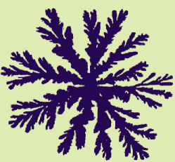
Figure 2.2: A typical ST aggregate.

The Laplacian growth models exhibit fingered fractal patterns as seen for example in figure (2.3) for DLA, or figure (2.1) for Hele-Shaw flows. The parts of the interface further away from the origin tend to move faster than the parts closer to the center. This instability causes the fingers (see Figure 2.2) to become more and more sharp until finally they form a cusp. Of-course in real experiments the cusp is cut-off by surface tension

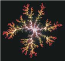
Figure 2.3: A typical DLA aggregate.

. Our approach is to study how quantization of the ST problem, may provide another method of regularization which keeps the integrability of the problem intact, and thus avoids the cumbersome mathematical complications presented by introducing surface tension [15] . This issue will be studied in later chapters, in the following sections we will discuss the mathematical description of the ST bubble.

2.1 Mathematical descriptions

In oder to analyze the evolution of, for example, the ST bubble, one needs first a mathematical tool to describe the shape of a this two-dimensional object. In this section we shall present two such mathematical methods: The first one is based on conformal mappings, while the second one employs the Schwarz function formalism.

To begin with, consider the univalent conformal mapping, $z(w;t)$, from the exterior of the unit circle, $|w|>1$, to the exterior of the bubble at time $t$, such that the unit circle $|w|=1$ is mapped to the interface contour, see Fig. 2.4. This mapping is assumed to have the following Laurent expansion:

$$z(w;t)=u_{1}(t)w+u_{0}(t)+u_{-1}(t)w^{-1}+u_{-2}(t)w^{-2}+...,$$ (2.3)

where the time dependence of the expansion coefficients $u_{i}(t)$ determine the evolution of the bubble in time. The form above is derived by demanding that the poles of the mapping reside inside the unit circle of $w$ plane, and that it is univalent in the exterior domain.

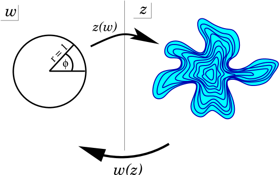
Figure 2.4: Mapping from the exterior of the unit circle, where the complex coordinate is denoted by $w$ to the exterior of the aggregate (where the coordinate is $z$).

Using the conformal mapping description it is easy to express the solution for the Laplace equation (2.2) as

$$P=\Re\left(\log\left(w\left(z\right)\right)\right),$$

where $w(z)$ is the inverse mapping. Indeed, $\log(w(z))$’s real part is a harmonic function satisfying Laplace equation. Moreover, it also satisfies the correct boundary conditions, $P=0$ on the interface. This is because the bubble contour is mapped to $|w(z)|=1$, consequently $\log w(z)$ is purely imaginary, and therefore its real part trivially vanish.

One may study the dynamics of the ST bubble by considering the evolution of the conformal map in time, $z(w;t)$. In fact, using the conformal mapping approach, D’Arcy’s law (2.1) takes a very appealing form - it can be written as the Poisson brackets of the conformal map, $z(w,t)$ and its complex conjugate $\bar{z}(w,t)$:

$$\{z(w;t),\bar{z}(w^{-1};t)\}=1,$$ (2.4)

where the canonical variables are $\log w$ and the time $t$ (which is also area of the bubble). To see that this is indeed a manifestation of D’Arcy’s law, (2.1), let us choose units where $b^{2}/12\mu$ is unity, and write it in the form

$$v_{n}=\left(\frac{\partial l}{\partial\theta}\right)^{-1}\left|\frac{\partial\vec{r}}{\partial t}\times\frac{\partial\vec{r}}{\partial\theta}\right|=-\frac{\partial P}{\partial n}$$ (2.5)

where $\vec{r}=(x,y)$ denote a point along the bubble contour, $\theta$ is the angle parameterizing the unit circle $\Im\log w=\theta$ (see Fig.  2.4), and $l$ is the arc length along the perimeter of the bubble. $\frac{\partial\vec{r}}{\partial t}$ is the velocity of a point on the contour. To obtain the normal velocity we take the cross product with the tangent $\frac{\partial\vec{r}}{\partial\theta}$, and then divide by the length of the tangent $\frac{\partial l}{\partial\theta}.$ Now using the Cauchy Riemann equations we get $\frac{\partial\theta}{\partial l}=\frac{\partial P}{\partial n}$, which implies:

$$\left|\frac{\partial\vec{r}}{\partial t}\times\frac{\partial\vec{r}}{\partial\theta}\right|=-1.$$

Writing the cross product in complex coordinates, and analytically continuing the equation away from the contour, we get (2.4) (where we also use the fact that the analytic continuation of $\bar{z}$ outside the perimeter of the bubble is $\bar{z}(w^{-1})$)

The second useful mathematical device we shall use in this work is the Schwarz function. To define the Schwarz function consider, first, an equation for the bubble interface (in the x-y plane) given by:

$$f(x,y)=0.$$

In terms of the complex coordinates, $z=x+iy$, $\bar{z}=x-iy$, we may rewrite this equation in the form

$$g(z,\bar{z})=f(\frac{z+\bar{z}}{2},\frac{z-\bar{z}}{2i})=0.$$

Then solving the equation $g(z,\bar{z})=0$ for $\bar{z}$ we obtain

$$\bar{z}=S(z).$$

$S(z)$ when analytically continued away from the perimeter of the bubble is known as the Schwarz function [16, 17, 18, 19]. Thus $S(z)$ is an analytic function which equals $\bar{z}$ on the bubble contour.

An important feature of the Schwarz function is its unitarity

$$z=\bar{S}(S(z)),$$ (2.6)

which follows from the fact that on the contour this condition is trivially satisfied, and since both sides of the equation represent analytic functions, the equality must hold all over the complex plane.

The relation between the Schwarz function and the conformal mapping description of the contour is

$$S(z)=\bar{z}\left(\frac{1}{w(z)}\right)$$

where $\bar{z}(w)$ is the complex conjugate mapping to $z(w)$ and $w(z)$ is the inverse mapping. This relation is derived by noticing that on the contour $w=e^{i\theta},$ $1/w=\bar{w}$, and $S(z)=\bar{z}(\bar{w})=\overline{z(w)}$.

2.2 Constants of motion

The ST dynamics in the absence of surface tension possesses an infinite number of conserved quantities known as the harmonic moments of the system[20]. These harmonic moments are defined as

$$t_{k}=-\frac{1}{\pi k}\int_{\mbox{visc.fluid}}\!\!\!\!\!\!\!\!\!\!\!\!d^{2}zz^{-k},k=1,2,\cdots,$$ (2.7)

where integration is over the viscous fluid (exterior) domain.

We give the proof that $\frac{dt_{k}}{dt}=0$, where $t$ is the time, which according to our convention will be equal to the area of the bubble. To show this, let us introduce the complex potential, $\Psi$, which is an analytic function such that $\Re(\Psi)=P$ is the pressure. Its imaginary part, $\theta=\Im(\Psi)$, known as the stream function goes to the polar angle as the distance from the origin goes to infinity since $P\sim\log(|z|)$. Thus by the Cauchy-Riemann equations $\frac{\partial P}{\partial n}=\frac{\partial\theta}{\partial l}$ where $n$ is the direction normal to the contour and $l$ is the direction along the contour. Therefore

$$\frac{d}{dt}t_{k}=-\frac{1}{\pi k}\frac{d}{dt}\int z^{-k}d^{2}z=-\frac{1}{\pi k}\oint z^{-k}\frac{\partial P}{\partial n}dl=$$

$$=-\frac{1}{\pi k}\oint z^{-k}\frac{\partial\theta}{\partial l}dl=\frac{i}{\pi k}\oint z^{-k}d\Psi,$$

where in the last equality we have used the fact that $\Psi$ is purely imaginary on the contour and thus $d\theta=-id\Psi$. Now by deforming the contour of integration such that it is a large contour around infinity, we see that the integrand vanishes quickly enough to render the integral $0.$ Finally, we remark that the above proof holds also for the case where there are more than one bubble of water.

Chapter 3 The Quantum Hall Effect

In the idealized setting, where no surface tension is present, the Saffman-Taylor problem confronts an obstacle. As a result of the scale invariance, some fingers develop cusp-like singularities within a finite time [21]. A modification of the growth law which introduces a mechanism curbing the curvature of the interface at a micro scale is necessary. The form (2.4) of the evolution equations, as Poisson brackets suggests to use a quantization procedure, whereby a Planck scale may be introduced which will serve as the small-scale cut-off for the theory. In this chapter we show [22] how the quantum Hall system in an inhomogeneous magnetic field serves as a quantization of the ST problem. In later chapters we will discuss the integrability of the quantum system, and the way it may be employed to find solutions of the ST problem, regularized by quantization.

We will study a shape of a large electronic droplet on the fully occupied lowest Landau level of a quantizing magnetic field. The magnetic field is assumed to be nonuniform in the area away from the droplet. We show that Aharonov-Bohm forces, associated with the nonuniform part of the magnetic field shape the edge of the droplet in a manner similar to a fingering interface driven by a Laplacian field.

In order to present our argument we shall neglect the interactions among the electrons and assume that the external electrostatic potential is zero. Under these conditions we will show that the semiclassical dynamics of the QH droplet is governed by the same equations of viscous fingering scaled to a nanometer scale. By the semiclassical limit we mean a large number of electrons $N\to\infty$, small magnetic length $\ell\equiv\sqrt{\hbar c/eB_{0}}\rightarrow 0$ but a finite area of the droplet ($\ell^{2}N\to const$). The droplets’ area is $\ell^{2}N$.

Let us first recall the physics of QH-droplets (see e.g., [23][24]). Consider spin polarized electrons on a plane in the lowest level of a quantizing nonuniform magnetic field, directed perpendicular to the plane, $B(x,y)>0$:

$$H=\frac{1}{2m}\left((-i\hbar\vec{\nabla}-\vec{A})^{2}-\hbar B\right).$$

The lowest level of the Pauli Hamiltonian is degenerate even for a nonuniform field. Aharonov and Casher[25] showed that the degeneracy equals the integer part of the total magnetic flux $\Phi=\int dxdyB$ in units of flux quanta, $\Phi_{0}=2\pi\hbar$ (we set $e=c=1$)[25, 26]. To see this define $A=A_{x}+iA_{y}$ and $\Pi=-2\hbar\partial_{\bar{z}}-i\bar{A}$. Then $H$ can be written as $H=\frac{1}{2m}\Pi^{\dagger}\Pi,$ assuming $\vec{\nabla}\cdot\vec{A}=0$. A zero energy solution $|\Psi\rangle$ would have

$$\left\langle\Psi\right|H\left|\Psi\right\rangle=\left\langle\Psi\right|\Pi^{\dagger}\Pi\left|\Psi\right\rangle=0\Rightarrow\Pi\left|\Psi\right\rangle=0$$

Thus, we may find the zero energy solutions, by solving the equation $\Pi\Psi=0.$ Since $H$ is a positive operator, these solutions would then belong to the ground state.

The equation $\Pi\Psi=0$ is first order and may be easily solved. A solution, $\tilde{\psi}_{m}(z),$ is given by:

$$\tilde{\psi}_{m}(z)=e^{-\frac{1}{2\hbar}V(\bar{z},z)}\tilde{P}_{m}(z),$$ (3.1)

where $\tilde{P}_{n}(z)$ is an arbitrary polynomials of a degree $n$. $V(\bar{z},z)$ is defined by the solution to the equation $B=\frac{1}{2}\nabla^{2}V$, given by

$$V(z,\bar{z})=\frac{1}{2\pi}\int\log(|z-z^{\prime}|^{2})B(z^{\prime})d^{2}z^{\prime}.$$

We may now choose a gauge by taking $A=i\partial_{z}V$.

In order for this formal solution to be an eigenvalue, it must be normalizable. As $|z|\longrightarrow\infty$, $P_{m}(z)\sim z^{m}$ and $V(z,\bar{z})\sim\Phi log(|z|),$ which gives $|\tilde{\psi}_{m}(z)|\sim|z|^{\left(m-\frac{\Phi}{\Phi_{0}}\right)},$ thus for normalizability we must have $m\leq\frac{\Phi}{\Phi_{0}}-1$. Thus the degeneracy of the level is $\frac{\Phi}{\Phi_{0}},$ a result obtained in [25, 26]. For later use let us define the orthogonal polynomials with respect to the measure $e^{-\frac{1}{\hbar}V(z,\bar{z})}$:

$$\int d^{2}xP_{n}(z)P_{m}(\bar{z})e^{-\frac{1}{\hbar}V(z,\bar{z})}=e^{\phi_{n}}\delta_{nm},$$

the orthogonal polynomials are assumed to be normalized such that their leading coefficient is 1, $P_{m}(z)=z^{m}+...$

We will consider the following arrangement: A strong uniform magnetic field $B_{0}>0$ is situated in a large disk of radius $R_{0}$; The disk is surrounded by a large annulus $R_{0}<|z|<R_{1}$ with a magnetic field $B_{1}<0$ directed opposite to $B_{0}$, such that the total magnetic flux $\Phi$ of the disk, $|z|<R_{1}$, is $N\Phi_{0}$. The magnetic field outside the disk $|z|<R_{1}$ vanishes. The disk is connected through a tunneling barrier to a large capacitor that maintains a small uniform positive chemical potential slightly above the zero energy of the lowest Landau level.

In this arrangement a circular droplet of $N$ electrons is trapped at the center of the disk $|z|<R_{0}$. We choose the magnetic field $B_{1}$ such that the droplet’s size, $\ell\sqrt{2N}$, is much smaller than the radius of the disk $R_{0}$.

Next we assume that a weakly nonuniform magnetic field $\delta B$ is placed inside the disk $|z|<R_{0}$ but well away from the droplet. The nonuniform magnetic field does not change the total flux $\int\delta Bdxdy=0$. The droplet grows when $B_{1}$ is adiabatically increased, keeping $B_{0}$, $\delta B$ and the chemical potential fixed. Then the degeneracy of the Landau level and, consequently, the size of the droplet increase.

For later reference it will be useful to write the potential $V(z,\bar{z})$ as:

$$V(z,\bar{z})=\frac{|z|^{2}}{2\ell^{2}}-W(z)-\overline{W(z)}.$$ (3.2)

The first term is associated with the uniform magnetic field of magnetic length $\ell,$ the second term is the associated with the non-uniform part of the total field, namely $\delta B$. Near the origin the field is uniform and thus $W$ is harmonic, and is given by:

$$W(z)=\sum_{k\geq 1}t_{k}z^{k},\;\;\;\;\;\;\;\,t_{k}=\frac{1}{2\pi k}\int\delta B(z)z^{-k}d^{2}z.$$

The parameters $t_{k}$ are, now, the harmonic moments of the deformed part of the magnetic field. Summing up, we have, around the origin,

$$V(z,\bar{z})=\frac{|z|^{2}}{2\ell^{2}}-\sum_{k\geq 1}\left(t_{k}z^{k}+\bar{t}_{k}\bar{z}^{k}\right).$$ (3.3)

From now on we will choose units in which the magnetic length is $\ell=\frac{1}{\sqrt{2}}.$

3.1 Coulomb gas

We will now show that the electrons occupy a region in space where the density is uniform - the electron droplet. Furthermore we will show that the droplet evolves according to the ST dynamics. The multi-particle wave function is given by a Slater determinant of wave functions of the form (3.1). The Slater determinant gives just a Vandermonde determinant, so that the normalization of the multi-particle wave function may be written as:

$$\tau_{N}=\frac{1}{N!}\int\prod_{i=1}^{N}d^{2}z_{i}\left|\det_{i,j}\left(P_{i}(z_{j})\right)\right|^{2}e^{-\frac{1}{\hbar}\sum_{i=1}^{n}V(z_{i},\bar{z}_{i})}=$$

$$=\frac{1}{N!}\int\prod_{i=1}^{N}d^{2}z_{i}\prod_{i>j}|z_{i}-z_{j}|^{2}e^{-\frac{1}{\hbar}\sum_{i=1}^{n}V(z_{i},\bar{z}_{i})},$$ (3.4)

where $\frac{1}{N!}$ is added for later convenience. We shall call this normalization factor “the $\tau$- function”. Let us now define the function

$$\psi_{m}(z)=P_{m}(z)e^{\frac{1}{\hbar}\left(-\frac{|z|^{2}}{2}+t_{k}z^{k}\right)}.$$ (3.5)

Then by the orthogonality of the polynomials, the $\tau-$function factorizes to:

$$\tau_{N}=\Pi_{m=0}^{N}\int|\psi_{m}(z)|^{2}d^{2}z=e^{\sum_{m=0}^{N}\phi_{m}}.$$

The factorization of the $\tau-$function is related to the fact that we are dealing with free fermions, i.e. the multi-particle wave function can be written as a Slater determinant of single-particle wave functions.

In understanding the relation between the quantum Hall setup described above and the ST problem it is instructive to adopt the view of Dyson’s gas [27] for the $\tau$-function. According to this picture, $z_{i}=x_{i}+iy_{i}$ denote the complex coordinate of the $i$-th particle, the Vandermonde determinant $\prod_{i>j}|z_{i}-z_{j}|^{2}$, when exponentiated, accounts for the logarithmic interaction between the particles, and $V(z,\bar{z})$ is the potential energy.

To find the density of Dyson’s gas, we write down the action of the Coulomb gas in terms of the density of the particles $\rho(z)=\sum_{i}\delta(z-z_{i})$:

$$S\left[\rho(z)\right]=-\int d^{2}z\left(\frac{1}{\hbar}V(z,\bar{z})\rho(z)-\int d^{2}z^{\prime}\rho(z^{\prime})\log(|z-z^{\prime}|)\rho(z)\right),$$

such that by varying this action with respect to $\rho(z)$,

$$\frac{1}{\hbar}V(z,\bar{z})-\int\rho(z^{\prime})\log(|z-z^{\prime}|^{2})=0,$$ (3.6)

and operating with the Laplacian on this equation we obtain:

$$\rho(z)=\frac{1}{\pi\hbar}\equiv\rho_{0}.$$

The last equation implies that the density of the eigenvalues is constant. However, the functional derivative makes sense only when $\rho>0$ since the density cannot be negative. Therefore, we expect that $\rho(z)=\rho_{0}$ only in the interior of some domain, $D_{+}$, and that it vanishes at the exterior of this domain, $D_{-}$.

Our purpose, now, is to show that $D_{+}$ and $D_{-}$ are indeed the interior and exterior domains of the ST bubble. For this purpose we shall show that the harmonic moments of $D_{-}$ are the $t_{k}^{\prime}s$ which enter in the potential. To show this, we will first show that $V(z,\bar{z})$ is the potential generated by a positive charge distributed uniformly in a region of harmonic moments $\{t_{k},\bar{t}_{k}\}$. Screening of this potential by Dyson’s gas (see equation (3.6)), which is assumed to be negatively charged, implies that Dyson’s gas is also distributed uniformly in a region of harmonic moments $\{t_{k},\bar{t}_{k}\}$.

Consider the potential generated by a positive charge, of density $1/\pi\hbar$, distributed uniformly in $D_{+}$:

$$\tilde{V}(z,\bar{z})=\frac{1}{\pi\hbar}\int_{D_{+}}d^{2}z^{\prime}\log\left|z-z^{\prime}\right|^{2}$$

Viewing this potential as the sum of a positive charge distributed uniformly in the whole plain and negative charge, of the same density, in the exterior domain, we may rewrite this potential as

$$\tilde{V}(z,\bar{z})=\frac{1}{\hbar}|z|^{2}-\frac{1}{\pi\hbar}\int_{D_{-}}d^{2}z^{\prime}\log\left|z-z^{\prime}\right|^{2},$$

where the first term account for the uniform charge density in the whole plain, while the second term accounts for the opposite charge density in the exterior domain. Notice that $z$ is located in the interior of the domain.

Now we expand the logarithm in powers of $\frac{z}{z^{\prime}}$ ( $z$ is in the interior domain while $z^{\prime}$ is in the exterior domain, and we expand in the small parameter $\frac{z}{z^{\prime}}$). Then up to an additive constant,

$$\tilde{V}(z,\bar{z})=\frac{1}{\hbar}|z|^{2}+2\Re\frac{1}{\hbar}\int_{D_{-}}d^{2}z^{\prime}\sum_{k=1}^{\infty}\frac{1}{\pi k}\left(\frac{z}{z^{\prime}}\right)^{k},$$

and from the definition of the harmonic moments (2.7) we arrive at (3.3). Thus Dyson’s gas occupy a domain of area $\pi\hbar N$ in the complex plane and whose harmonic moments are the set $\{t_{k},\bar{t}_{k}\}$. Thus the evolution of this domain, while increasing its area is precisely the evolution of ST bubble in the absence of surface tension.

It is interesting to compare dimensionless viscosity of liquids used in viscous fingering experiments [28][29], and a ”viscous” effect of quantum interference of at the first Landau level. The parameter of the dimension of length controlling viscous fingers in fluids is $\frac{2\pi}{q}\frac{b^{2}}{12\eta}\sigma$, where $q$ is the flow rate, $b$ is the thickness of the cell, $\eta$ is the viscosity and $\sigma$ is the surface tension. In recent experiments[28][29] , this length stays in high hundred of nanometers, but can be decreased by increasing the flow rate. This length is to be compared with the magnetic length $\ell$. At magnetic field about 2T it is about 50 nm. Semiconductor devices imitating a channel geometry of the original Saffman-Taylor experiment [1] may facilitate fingering instability.

3.2 Relation to the 2d Toda lattice equations.

An interesting feature of the quantum Hall problem described above is that the $\tau-$function , $\tau_{n}=\prod_{m=0}^{n}e^{\phi_{m}},$ satisfies the integrable nonlinear equation [2, 30, 31, 32, 5, 33], associated with the 2d Toda lattice (2DTL).:

$$\frac{\partial^{2}}{\partial t_{1}\partial\bar{t}_{1}}\log\left(\frac{\tau_{n}}{\tau_{n-1}}\right)=\frac{\tau_{n-1}^{2}}{\tau_{n-2}\tau_{n}}-\frac{\tau_{n}^{2}}{\tau_{n-1}\tau_{n+1}},$$ (3.7)

where $t_{1}$ is the time (here assumed to be a complex number) and $n$ is an integer which can be regarded as a discretized coordinate of space (see appendix A for a proof). This equation is a natural extension of the one dimensional Toda lattice where $t_{1}$ is real. The full hierarchy of nonlinear equations can be derived from the Lax equations which are derived in appendix C. In the next chapter we will discuss how the quantized system may be treated as a regularization of the ST system. We will use methods from the study of classical integrable systems to describe this regularization.

Chapter 4 Dispersive regularization

In the previous chapter we established the relation between the 2DTL and the ST problem. The purpose of this chapter is to study the implementation of a method known as dispersive regularization [34, 35, 36]. We shall borrow methods from soliton theory in order to find solutions to the 2DTL and find their classical analogue which describe the ST bubble. As was explained, the need for regularization in the ST problem arises from the appearance of cusps in the shape of the bubble, in finite time, for generic initial conditions. Surface tension, in this respect, is the most natural candidate, since no matter how small it is, as long as it is nonzero, it hinders the formation of a cusp . Indeed, the real system avoids cusps by repeated processes of tip splittings. Yet, the introduction of surface tension destroys the integrable structure of the idealized problem, and any analytic treatment becomes a complicated task[15].

We suggest using dispersive regularization as an alternative method by which the dynamics of the idealized problem can be continued beyond the cusp, for some large set of initial conditions. This is the set which can be associated with the cases where the cusp forms due to the merging of the initial bubble with another small bubble, as illustrated in Fig. 4.1. In other words, dispersive regularization is an extension of the ST dynamics in which more than one bubble may exist, for small time intervals, and the evolution passes through repeated events of formation of new bubbles which merge with the original one.

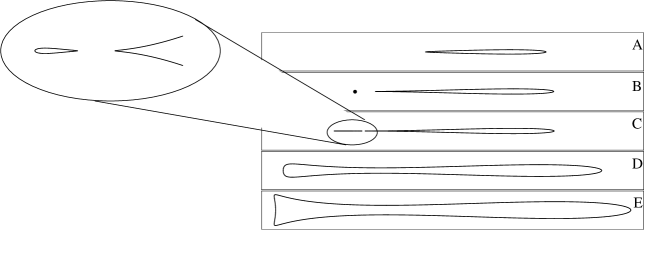
Figure 4.1: Evolution of the droplet regularized by the addition of a droplet. Panel A shows a single bubble. Panels B and C show an additional bubble forming near the tip of the first droplet. In panel D the two bubbles have merged to form a single bubble again.

In the general context dispersive regularization is a method for finding approximate solutions for nonlinear wave equations, such as the KdV equation (where it is also known as the Gurevich-Pitaevskii method [37, 34]). The application of dispersive regularization to the ST problem follows from the observation that the equations governing the latter problem are the saddle point equations of the two dimensional Toda lattice (2DTL). Putting it differently, ”quantization” of the ST problem leads to the 2DTL. Thus, using dispersive regularization one can construct approximate solutions for the 2DTL, and taking the saddle point approximation (equivalent to the quasi-classical limit) yields general solutions for the ST problem, see the flow diagram in Fig. 4.2. As we will show some of the solutions obtained via dispersive regularization describe situations where the system may consists of more than one bubble, as illustrated in Fig. (4.1). These turn out to be exact solutions of the multi-bubble generalization of the ST problem.

In this chapter we will first discuss the simpler case of the KdV equation. Then we show how to generalized the method for the 2DTL. In Chapter 5, following Richardson, we develop an alternative, equivalent, method for describing the evolution of ST bubbles. As we will show the solutions of the equations may not comply with the ST dynamics - a situation which refer to as “virtual bubble” solutions, see Fig. 4.2. We will discuss these virtual bubbles and explain their behavior by employing a physical viewpoint based on the description of the ST problem as a noninteracting fermion system. In chapter 6 we show how to construct general two-bubble solutions for the ST problem, and describe their evolution. We hall also explain how these solutions resolve the problem of cusp-like singularities.

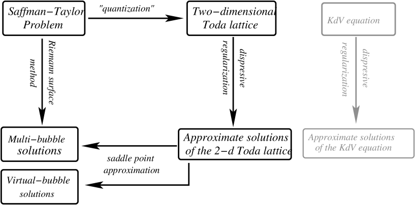
Figure 4.2: Flow chart for organization of chapters 4-6. We find solutions of the 2DTL by the dispersive regularization approach which leads to the introduction of multi-bubbles solutions for the ST dynamics. We also discuss the role of virtual bubbles in the solutions thus found. We introduce some of the methods which are used in this article in the settings of the KdV equations and use the analogy to the 2DTL to gain insight to the ST problem.

4.1 Dispersive regularization for the KdV Equation

Dispersive regularization is a general method for calculating approximate solutions for nonlinear wave equations, for a large set of initial conditions. Conceptually, it consists of two stages: In the first stage a set of exact solutions for the nonlinear wave equation is constructed. These solutions depends on parameters, $\{\lambda_{i}\}$, which are, in fact, constants of motion of the problem. In the second stage, this set of solutions is used as an approximate local description of more general solutions, by allowing the parameters $\{\lambda_{i}\}$ to have slow time and space dependences. Thus the aim of this section is to construct solutions for the 2DTL using the dispersive regularization approach. It will be instructive, however, to overview first the milestones of this approach for the simpler case of the KdV equation[38]. We shall begin this section by describing the analogy between the KdV system and the ST problem. then we shall consider the inverse scattering approach, which will allow us to construct modulated oscillatory solutions for the KdV equation, the equations for the modulated waves, known as the Whitham equations will be discussed next.

The KdV (Korteweg de-Vries) equation,

$$u_{t}-6uu_{x}-\beta u_{xxx}=0,$$ (4.1)

is a nonlinear one-dimensional wave equation devised in order to model water waves is a shallow canal. Although very different from the ST problem considered in this thesis, the dynamics of the KdV equation is, in some sense, analogous to our problem. To clarify this analogy consider the evolution of $u(x,t)$ in the absence of dispersion $(\beta=0)$,

$$u_{t}-6uu_{x}=0.$$

with general initial conditions:

$$u(x,t=0)=f(x).$$

The Riemann solution for this problem is given by the implicit form:

$$u(x,t)=f(x+6u(x,t)\cdot t).$$ (4.2)

However, this solution for a general function $f(x)$ becomes non-physical beyond some finite time: It develops overhangs as illustrated in Fig. (4.3). The dispersive term, however small it is, hinders such situations since as the system approaches a overhang the dispersive term $u_{xxx}$ diverges. Indeed, instead of overhangs the system develops oscillations as demonstrated in Fig. (4.3).

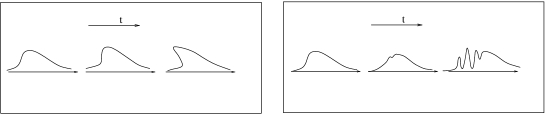
Figure 4.3: left panel shows the evolution of the dispersionless KdV equations, while the right panel shows the effect of dispersion which replaces the overhang with an oscillatory region.

The analogy between the KdV equation and ST problem is summarized in Fig. (4.4). The dispersionless KdV equation is analogous to the ST problem in the absence of surface tension; Overhangs are analogous to cusps; And the dispersive KdV equation is analogous to the 2DTL.

Figure 4.4: Table showing analogy between the KdV equations and the ST dynamics. The dispersionless KdV which is analogous to the ST problem develops overhangs in much the same way as the ST dynamics develops cusps. The resolution of this problem may be achieved in the KdV equations by the introduction of dispersion, which is analogous to finding dispersively regularized solutions of the 2DTL.

We turn now to describe how dispersive regularization resolves the problem of overhangs. The first stage is the construction of a set of exact solutions for the problem. This construction, is based on the remarkable fact that if a solution $u(x,t)$ of the KdV equation is considered as a time-dependent potential in a Schröedinger operator,

$${\mathcal{H}}=-\frac{d^{2}}{dx^{2}}+u(x,t),$$

then the resulting spectrum of the equation

$${\mathcal{H}}\psi_{\lambda}=\lambda\psi_{\lambda}$$

is independent of time, $(d\lambda/dt=0)$.

Thus one may assume a given form of the eigenvalue-spectrum, as well as some analytic properties of the wave function (the “scattering data”), and try to construct the corresponding potential $u(x,t)$ (i.e. the “scattering potential”). This reconstruction of the potential from the scattering data is known as the inverse scattering approach.

The idea is first to construct eigenfunction $\psi_{\lambda}$, as a the Baker-Akhiezer (BA) function, from its analytic properties as function of $\lambda$. Then the potential (which is the solution of KdV equation) is straightforwardly extracted by substitution into the Schröedinger equation:

$$u(x,t)=\frac{1}{\psi_{\lambda}}\frac{d^{2}\psi_{\lambda}}{dx^{2}}+\lambda$$ (4.3)

Inverse Scattering

To demonstrate this inverse scattering approach, let us consider, first, the simplest situation where $u(x,t)=u_{0}$ is a constant depending neither on time nor a space (this is clearly a trivial solution of the KdV equation). The spectrum in this case is continuous for $\lambda>u_{0}$, and the corresponding eigenfunction takes the form $\psi_{\lambda}=e^{\pm i\sqrt{\lambda-u_{0}}x}$. Thus for general complex parameter, $\lambda$, there are two solutions $\psi_{\lambda}^{(+)}$ and $\psi_{\lambda}^{(-)}$ corresponding to the two values of the square root function. These solutions have branch cuts which may be taken to coincide precisely with the spectrum.

Instead of considering the eigenfunctions, $\psi_{\lambda}$ to be a multi-valued function of $\lambda$, we may define a Riemann surface over which the BA function is single valued: We may take two copies of the complex plane with branch cuts along the ray $\lambda>u_{0}$ and assign the value $e^{i\sqrt{\lambda-u_{0}}x}$ , on one copy and $e^{-i\sqrt{\lambda-u_{0}}x}$ on the other. We can now cut the two copies of the complex plane along the branch cut and glue the upper part of the branch cut of one sheet to the lower part of the branch cut on the other sheet (and vice versa) so that now $\psi_{\lambda}$ is a smooth function on the Riemann surface obtained by this cut and paste procedure (see Fig. 4.5). One can also assign proper coordinate systems around each point so that the surface has the structure of a Riemann surface. This is done by choosing a coordinate system $\lambda^{-\frac{1}{2}}$ around the infinities, $\sqrt{\lambda-u_{0}}$ around the branch cuts, and $\lambda-\lambda_{0}$ near a general point $\lambda_{0}$. The Riemann surface obtained by this method is the algebraic Riemann surface associated with the equation $y^{2}=\lambda-u_{0}$. We shall generally refer to the Riemann surface associated with the Hamiltonian ${\mathcal{H}}$ as the spectral surface.

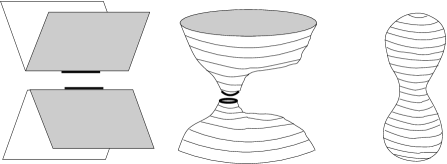
Figure 4.5: Construction of a genus-0 Riemann surface: On the left the two sheets of the Riemann surface are presented with branch cut in heavy line. In the middle figure, the two sheets are deformed and the branch cuts are opened up. The drawing on the right shows the surface which is obtained by pasting the two surfaces along the branch cuts and after compactification have been performed (by incorporating the infinities in the Riemann surface.

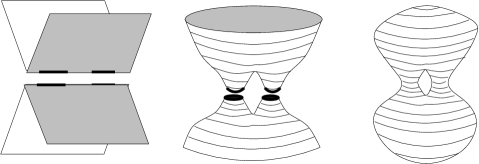
Figure 4.6: Schematic drawing of construction of genus-1 Riemann surface, from the curve $y^{2}=\Pi_{i=1}^{4}(z-\lambda_{i})$.The construction is analogous to that demonstrated in Fig 4.5.

Consider now a more general situation where the eigenvalue spectrum of ${\mathcal{H}}$ consists of disconnected pieces, or in other words, the spectrum has a finite number of gaps. Our goal, now, is to calculate the corresponding BA function from which we can deduce the potential $u(x,t)$, according to equation (4.3). Our strategy is to construct, first, the corresponding Riemann surface over which the BA function is single valued, and then to deduce its form from the analytic properties on this surface, together with a choice of normalization.

In understanding the structure of the spectral surface for finite gap solutions, it is important to notice that it is always composed of two Riemann sheets. This follows from the property that the Schröedinger operator ${\mathcal{H}}$ is of second order. If we denote by $\lambda_{i}$ the endpoints of the pieces of the spectrum, then the spectral surface has the form: $y^{2}=\Pi_{i=1}^{2m+1}(\lambda-\lambda_{i})$, where $m$ is the number of gaps. Such a Riemann surface is called hyper-elliptic see Fig. 4.6.

The BA function may now be constructed by demanding proper analytic behavior on this hyper-elliptic Riemann surface, and that in the large $\lambda$ limit it takes the asymptotic form

$$e^{\pm i\sqrt{\lambda}x},$$

a behavior which reflects an essential singularity at $\lambda\rightarrow\infty$, on both Riemann sheets. We defer these details to Appendix B. We just mention the result that the finite gap solutions of the KdV equation obtained by this method have the form of quasi-periodic traveling waves

$$u(x,t)=u(kx+\omega t;\{\lambda_{i}\}),$$ (4.4)

where the wavenumber $k(\{\lambda_{i}\})$ and the frequency $\omega(\{\lambda_{i}\})$ are functions of the branch points, $\{\lambda_{i}\}$.

Whitham equations

We showed above how to construct a set of finite gap solutions for the KdV equation, by the inverse scattering method. Our next step is to sew together these solutions to approximate more general cases. Namely, we would like to use exact solutions found in the previous stage as a local (space-time) description of a general function, as illustrated in Fig.  (4.3).

Since the solutions of the KdV equation (4.4) are uniquely determined by the values of branch points, $\{\lambda_{i}\}$ one may generalize these solutions by endowing these branch points a slow time and space dependence. A more general solution having this property is

$$u(x,t)=u(S(x,t);\{\lambda_{i}\})$$

where the set $\{\lambda_{i}\}$ which determines the form of the solution, is slowly changing in space and time, and the function $S(x,t)$ replaces the argument $k\cdot x+\omega\cdot t$ of the exact solutions. To ensure that this solution is locally described by one of the exact solution we demand that the first order expansion of $S(x,t)$ reproduce the argument of the finite gap solutions, thus

$$\frac{\partial S}{\partial x}=k(\{\lambda_{i}\})\leavevmode\nobreak\ \leavevmode\nobreak\ \leavevmode\nobreak\ \leavevmode\nobreak\ \leavevmode\nobreak\ \leavevmode\nobreak\ \leavevmode\nobreak\ \frac{\partial S}{\partial t}=\omega(\{\lambda_{i}\}).$$ (4.5)

where $k(\{\lambda_{i}\})$, and $\omega(\{\lambda_{i}\})$ are the wave number and frequency of the KdV solution characterized by the set $\{\lambda_{i}\}$. For constant $\{\lambda_{i}\}$, these equations trivially reduce to the finite gap solutions (4.4). However, when $\{\lambda_{i}\}$ have slow time and space dependences, these equations, known as the Whitham equations, yield a more general behavior which is described by slow evolution of the finite gap solutions. The treatment above of the Whitham equations may only be considered as a motivation, while the rigorous proof of these equations usually proves more technically involved[35, 39].

The evolution of the branch points $\{\lambda_{i}\}$ as function of the time can be deduced from the compatability condition for Whitham equations,

$$\frac{\partial k(\{\lambda_{i}\}}{\partial t}=\frac{\partial\omega(\{\lambda_{i}\}}{\partial x}.$$ (4.6)

Thus, given initial conditions of the KdV equation, $u(x,t=0)$, one can calculate the set $\{\lambda_{i}(x,t=0)\}$ and hence the evolution in time $\{\lambda_{i}(x,t)\}$. Then solution of the Whitham equations yield the approximate solution (4.4) for any time $t$.

By this approach the complicated problem of describing general solutions for the initial value problem of the KdV equation (which in general depends on a very large set of constant $\lambda_{i}^{\prime}$s) has been approximated by equations for a small number of parameters, which are the branch points of the Riemann surface. These equations which describe the evolution of spectral surface, allow for appearances and disappearances of gaps in the spectrum, i.e. changing the genus of the spectral surface.

Thus by dispersive regularization, one may obtain solutions for the KdV equation which are relevant also for long times, and which do not exhibit the singular behavior of the Riemann solution. These solutions display a breakup of the wave into oscillations (described by finite gap solutions) near points where the dispersion term, $u_{xxx}$ becomes large. A gap in the spectrum is opened up when the system approaches an overhang. Near this space-time point the behavior is described by a genus one surface, associated with the oscillatory behavior. Far from this point, where the Riemann solution (4.2) gives a good approximation, the corresponding spectral surface is of genus zero.

4.2 The 2d Toda Lattice equations

Our purpose now is to use dispersive regularization approach to find solutions of the 2DTL. This is the central part of this chapter and it will be organized as follows: We first present the spectral equation associated with the 2DTL, then discuss the meaning of the BA function and show that this function defined in the complex plane is peaked along the contour of the ST bubble. Next we construct the spectral surface, and present the general procedure for constructing the BA function based on the Krichever approach [40]. Finally we will show that this procedure is equivalent to the Whitham equations.

The spectral equation

As explained above, the dispersive regularization approach is based on the existence of a related spectral equation. Indeed, there is such an equation for the 2DTL, which is similar to that of the KdV,

$${\mathcal{L}}\vec{\psi}=z\vec{\psi},$$ (4.7)

but in contrast with the KdV case, where the spectral operator (the Schröedinger operator) is Hermitian, here the operator ${\mathcal{L}}$ is non-Hermitian, and the analogue of the eigenvalue spectrum assumes general complex values, $z$.

The noninteracting fermion picture of the 2DTL provides a simple way for understanding the meaning of the spectral equation - it reflects the recursion relations of the corresponding orthogonal polynomials, $P_{m}(z)$[41]. To explain this, let us choose the single particle wave functions, $\psi_{n}(z)$ to be the elements of the BA function, which in our case should be viewed as a vector:

$$\left(\vec{\psi}\right)_{n}=\psi_{n}(z)=P_{n}(z)e^{\frac{1}{\hbar}\left(-\frac{|z|^{2}}{2}+t_{k}z^{k}\right)}.$$

Multiplying $\psi_{n}(z)$ by $z$ results in the replacement of $P_{n}(z)$ by another polynomial $zP_{n}(z)$. Since $zP_{n}(z)$ can be written as a sum of the orthogonal polynomials of degree $m\leq n+1,$ we have:

$$z\psi_{n}(z)=\psi_{n+1}+a_{n,n}\psi_{n}+a_{n,n-1}\psi_{n-1}...+a_{n,0}\psi_{0}.$$

which can be recast in vector form as the spectral equation (4.7). where the matrix elements of $\mathcal{L}_{mn}=a_{nm}$ form a triangular matrix, since ${\mathcal{L}}_{nm}=0$ for $m>n+1$. In appendix C we prove that this construction of ${\mathcal{L}}$ indeed satisfies the conditions required in order to be considered as the Lax operator of the 2DTL.

A different view of the spectral operator employs the quantization relation between the ST problem and the 2DTL. Namely the spectral operator ${\mathcal{L}}$ may be considered as the operator associated with quantization of the classical conformal mapping (2.3). This quantization follows form the identification of $\log(w)$ and the time $t$ as classical conjugate variables, as discuss in Sec. 2.1. Thus demanding non-vanishing commutation relations between them, $[\log(w),t]=i\hbar$ allows representing $\log(w)$ as $i\hbar\partial_{t}$, and from expression (2.3) for the conformal mapping we have,

$${\mathcal{L}}=z\left(e^{i\hbar\frac{\partial}{\partial t}}\right)=u_{1}e^{i\hbar\frac{\partial}{\partial t}}+u_{0}+u_{-1}e^{-i\hbar\frac{\partial}{\partial t}}+u_{-2}e^{-i2\hbar\frac{\partial}{\partial t}}+...$$ (4.8)

Notice that this expression for the spectral operator agrees with the triangular form of the matrix ${\mathcal{L}}_{nm}$ discussed above, since $e^{i\hbar\frac{\partial}{\partial t}}$ is a shift operator

$$\left(e^{i\hbar\frac{\partial}{\partial t}}\vec{v}\right)_{t}=\vec{v}_{t+\hbar}.$$

and $t=\pi\hbar n$ is the area of the droplet containing $n$ fermions.

Thus in the dispersionless limit, $\hbar\rightarrow 0$, ${\mathcal{L}}$ reduces to the conformal mapping $z(w;t)$. Moreover the relation $\{z(w;t),\bar{z}(w;t)\}$ suggests that the spectral operator satisfies analogous quantum relation, known as the string equation[42]:

$$[{\mathcal{L}},{\mathcal{L}}^{\dagger}]=\hbar.$$ (4.9)

Notice that the string equation, which will be proved in Appendix C, imposes an additional constraint on the form of the spectral operator of the 2DTL. This constraint selects a subset of solutions out of the general solutions of the 2DTL, as we expect the corresponding eigenfunction, $\psi_{n}(z)$, to be associated with the shape of the classical bubble.

The Baker Akhiezer function of the 2DTL

As we saw above, the spectral equation can be thought as a quantization of the conformal map formalism. Below we take a closer look at the wave functions $\psi_{n}(z)$ themselves and see that they already encode the shape of the bubble in the ST evolution in a quite natural way. The consequence of this will be that the spectral surface ($z$ plane) can be identified as the physical plane (the 2D plane on which the physical evolution takes place), in contrast with the KdV case where the spectral surface served only as an auxiliary mathematical construction.

We begin by arguing that the $N$-th component of the BA function, i.e. $\psi_{N}(z)$, is peeked along the contour of ST bubble of area $\pi\hbar N$. Consider the particle density associated with the noninteracting fermionic systems, which is a sum over the single particle densities:

$$\rho(z)=\sum_{n=1}^{N}|\tilde{\psi}_{n}(z)|^{2},$$

where $\tilde{\psi}_{n}(z)$ denote the normalized $\psi_{n}(z)$ (namely $\int d^{2}z|\tilde{\psi}_{n}(z)|^{2}=1$). As we showed in Section 3.1, using Dyson’s gas picture, this density, in the limit $\hbar\to 0$, $N\rightarrow\infty$ keeping $\hbar N$ constant, vanishes outside the ST bubble and is constant within the bubble. Moreover, we have shown that by increasing the number of fermions $N$, the droplet area increases in accordance with the ST dynamics, i.e. keeping the harmonic moments, $\{t_{k},\bar{t}_{k}\}$ constant. Therefore the last particle added to the droplet must be distributed along the droplet perimeter, i.e. $\tilde{\psi}_{N}(z)$ is peeked along the contour of ST bubble of area $\pi\hbar N$.

Thus, in the dispersionless limit we expect the BA function to have the form

$$\psi(z)\sim e^{-\frac{1}{\hbar}\left(\frac{1}{2}|z|^{2}-\int dzS(z)\right)},$$ (4.10)

where $S(z)$ is the Schwarz function of the ST bubble. This form emerges because the saddle manifold, where the modulus of this function assumes its maximal value, is the droplet contour $\bar{z}=S(z)$. Thus by constructing the BA function of the 2DTL on various types of spectral surfaces, and looking at its saddle manifolds as function of $\pi\hbar N$ (which is the bubble area $t$) we expect to be able to extract the regularized dynamics of the ST problem.

To further clarify the analytic structure of the BA function, consider its form given by the formula,

$$\psi(z)=\psi_{N}(z)=e^{-\frac{1}{\hbar}\left(\frac{|z|^{2}}{2}-\sum_{k}t_{k}z^{k}\right)}P_{N}(z),$$

where $P_{N}(z)$ denotes the orthogonal polynomial of problem as discussed in Sec. 3.1. Since this polynomial is of order $N$, it has $N$ roots associated with $N$ zeros located in the complex plane. Thus lifting the polynomial $P_{N}(z)$ to the exponent

$$\psi(z)=e^{-\frac{1}{\hbar}\left(\frac{|z|^{2}}{2}-\sum_{k}t_{k}z^{k}\right)+\log(P_{N}(z))},$$

and comparing to the expected form of the BA function (4.10), we conclude that $S(z)$ has a pole singularity at each zero of the polynomials.

When $N\rightarrow\infty$ the number of zeros of $P_{N}(z)$ becomes infinite, and a well defined limit for their distribution is reached when $\hbar\rightarrow 0$ keeping $\hbar N$ constant. In this limit the zeros of the polynomial may be described by a line density on a set of contours in the complex plane. These lines may form the branch cuts of $S(z)$, which are analogous to the spectrum in the KdV problem.

The spectral surface

Since the BA function determine the shape of the ST bubble, our goal now is to compute this function and describe its evolution in time. For this purpose we shall employ the dispersive regularization approach as was done for solving the KdV equation. Namely, we will reduce the problem to the evolution of the spectral surface (i.e. to the evolution of its branch points). This procedure amounts to the assumption that the Schwarz function, $S(z)$, is an algebraic function, namely it is defined on an algebraic Riemann surface, defined by an equation of the form $Q(z,y)=0,$ where $Q$ is a polynomial in its both arguments, e.g. $Q(z,y)=y^{2}-\prod_{i=1}^{4}(z-\lambda_{i})$.

In order to construct the Riemann surface from this polynomial, one first solves the equation $Q(z,y)=0$ for $y$. The resulting function, $y(z)$, is multi-valued due to the presence of roots in the solution (e.g. $y=\sqrt{\Pi_{i=1}^{4}(z-\lambda_{i})}$ in the example above). In general there will be $n$ solutions of $y$ for each $z$. Thus one may introduce $n$ copies of the complex plane, where each copy is associated with a well defined value $y(z)$. Clearly, on each copy of the complex plane $y(z)$ is discontinuous along the branch cuts. To make it continuous we may paste together the various sheets of the complex plane along the branch cuts. Then, together with a choice of local coordinate systems around each point one obtains a Riemann surface composed of $n-$sheets glued together along the branch cuts, similar to the construction demonstrated in Fig. (4.6).

To each point on the Riemann surface, we have constructed, we would like to assign a value of the Schwarz function, $S$. In order to specify a point on the Riemann surface we must indicate an index $i$ (where $1\leq i\leq n$), and a complex number $z$. The index, $i$, will specify on which copy of the complex plane the point lies, and a complex number, $z$, will specify the coordinate on that copy. There will be one copy of the complex plane, which will be termed as “the physical sheet”, on which the bubble lies. On this Riemann sheet $S(z)$ will be equal to $\bar{z}$ on the perimeter of the bubble. On the other copies of the complex plane, $S(z)$ should be understood as an analytic continuation of $\bar{z}$.

Construction of $S(z)$

The next step of the dispersive regularization approach is the construction of the BA function which in our case is equivalent to the construction of the Schwarz function, $S(z)$. Two conceptual steps constitute this construction. First, the identification of the singular behavior of $S(z)$ outside the bubble (on the physical sheet). This is done using the relation

$$S(z)\sim\sum_{k=1}^{\infty}kt_{k}z^{k-1}+\frac{t_{0}}{z}$$ (4.11)

which holds for large $z$ outside the bubble, where $t_{k}$ and $t$ are the harmonic moments and the area of the bubble respectively. The above relation follows from the definition of harmonic moments (2.7) which by using Green’s theorem implies that

$$t_{k}=-\frac{1}{\pi k}\int_{D_{-}}\frac{d^{2}z}{z^{k}}=\frac{1}{2i\pi k}\oint dzS(z)z^{-k},$$ (4.12)

where the contour integral is taken along the bubble perimeter. By deforming the contour on the physical sheet one can verify that $S(z)$ must satisfy (4.11). Notice that by definition of the physical sheet, the deformation of contour does not cross any branch cuts. If there are no singularities of $S(z)$ except at infinity, a similar argument shows that $t_{0}$ is equal to the area of the bubble $t$: $t_{0}=t=\int_{D_{+}}d^{2}z$.

The second step is to identify the singularities of $S(z)$ on the other parts of the Riemann surface (including all non-physical sheets). This is achieved using the unitarity condition $z=\bar{S}(S(z))$. Recall that the Schwarz function maps the region outside the bubble onto the region inside the bubble which includes all non-physical copies of the complex plain. Thus knowing the analytic properties of $S(z)$ and the structure of the Riemann surface one may construct $S(z)$ and in particular its dependence on the parameters $t_{k}$ as well as in their anti-holomorphic counterparts, $\bar{t}_{k}$, and the area $t$.

We turn now to describe how the above procedure is implemented in practice. For this purpose it is more convenient to construct the differential $\hat{S}=S(z)dz$ and then deduce the Schwarz function from the relation $S(z)=\hat{S}/dz$.

We begin by identifying all singular points of the Riemann surface. To this end we use formula (4.11) on the physical sheet, outside the bubble, and the unitarity condition, $z=\bar{S}(S(z))$, to reveal the singularities inside the bubble including the non-physical sheets. The next step is to associate with the singular points meromorphic differential, on the Riemann surface, $\hat{\omega}_{i}$ which comply with a given singular structure at these points. The differential $\hat{S}$ is then obtained as the sum of these meromorphic differentials.

The meromorphic differentials on a Riemann surface, $\hat{\omega}_{i}$, are defined uniquely, given their singular structure (analytic behavior around the poles of the Riemann surface) and their normalization. This normalization is determined by the integral of $\hat{\omega}_{k}$ around cycles of the Riemann surface. Below, we shall elaborate on this point. For the time being we shall only state that different choices of this normalization amounts to different choices of the types of evolution of the ST dynamics.

For an arbitrary Riemann surface the procedure above will produce a function which satisfies the unitarity condition around the singular points, but in general will not satisfy the unitarity condition globally. But if the Schwarz function exists on a given Riemann surface the procedure above must produce this function. Thus to obtain a Schwarz function for a given set of harmonic moments, we must first find the Riemann surface on which it is defined, in other words we must find the location of the branch points (which determine the Riemann surface uniquely if we also know how the different sheets are interlaced).

To find the location of the branch points we may use the fact that unitarity must be satisfied around the branch points. This leads on fairly general conditions to the conclusion that $S(z)$ may not diverge at the branch points. This property alone will be enough to find the location of the branch points. To show that the Schwarz function does not diverge at the branch points, we assume that $\overline{S(z)}$ maps the exterior of the bubbles to the interior, where the interior also includes the unphysical sheets. We also assume that all branch cuts are in the interior. If we assume that $S(z)$ diverges on a branch points, $\lambda_{i}$, then $\overline{S(z)}$ will also diverge on the branch point. This in turn implies, by unitarity, that $S(z)$ has the following form around infinity:

$$S(z)\sim\bar{\lambda}_{i}+O(z^{-1}).$$

Which gives that $t_{1}=\bar{\lambda}_{i}$. Thus we have that $S(z)$ diverges on a branch point only for special choices of the harmonic moments.

Let us look at the implication of the non-divergence property of $S(z)$ near the branch points. Consider the Schwarz function, $S(z)=\hat{S}/dz$. Near one of its branch points, the local coordinate is $\delta=\sqrt{z-\lambda_{i}}$ and therefore $dz=2\delta d\delta$. Since $\hat{S}$ is meromorphic, near the branch point it can be expanded as $\hat{S}\simeq a_{1}d\delta+a_{2}(d\delta)^{2}+...$, and therefore $S(z)=\hat{S}/dz\sim a_{1}/\delta=a_{1}/\sqrt{z-\lambda_{i}}$. The requirement that $S(z)$ is not singular near the branch points implies that $a_{1}=0$. This condition may be recast as follows:

$$\oint\frac{S(z)dz}{\sqrt{z-\lambda_{i}}}=0,$$ (4.13)

where the integral is over small circles around each one of the branch points of the Riemann surface. The number of conditions which these integrals gives is the same as the number of branch points, which is enough to fix the form of the Riemann surface. Eq. (4.13), which is the central result of this section, has been constructed in different context by Krichever [43]. It gives the evolution of the spectral surface as a function of the times. From this information one can deduce the behavior of the Schwarz differential, $\hat{S}\equiv S(z)dz$, and obtain the time dependence of Schwarz function which describes the bubble dynamics.

Example: One Miwa variable on genus-0 surface

Let us consider an example in order to demonstrate the procedure described above. We focus on the case where the set of harmonic moments is given by:

$$t_{k}=\frac{\mu}{k}q^{-k}$$

for $k>1$, and for $k=1$

$$t_{1}=t^{\prime}_{1}+\frac{\mu}{q}$$

where $\mu$ is real, while $t^{\prime}_{1}$ and $q$ are arbitrary complex numbers. From formula (4.11) which holds outside the bubble we have

$$S(z)=\frac{t_{0}}{z}+t^{\prime}_{1}+\mu\sum_{k=1}^{\infty}\frac{z^{k-1}}{q^{k}}$$

and summing over $k$ yields

$$S(z)\sim\frac{t_{0}}{z}+t^{\prime}_{1}-\frac{\mu}{z-q}\leavevmode\nobreak\ \leavevmode\nobreak\ \leavevmode\nobreak\ \leavevmode\nobreak\ \leavevmode\nobreak\ \leavevmode\nobreak\ \mbox{in the exterior domain}$$

Thus Schwarz function has a simple pole at $q$ with residue $\mu$. Since now $S(z)$ has an additional singularity at the point $q$, the equality $t_{0}=t$ (where $t$ is the area of the bubble). In fact one may derive $t_{0}=t-\mu$. The pole of $S(z)$ in the the exterior domain is called “Miwa variable”[44, 45, 46, 47, 48, 49, 50, 51, 52]. It is characterized by its location, $q$ and weight $\mu$. The case of one Miwa variable is one of the simplest nontrivial cases to consider.

Having assumed the singular structure at the exterior of the bubble we may now use the unitarity condition, $\bar{S}(S(z))=z$, to find the singular structure in the interior of the bubble . Consider the limit $z\rightarrow\infty_{+}$, where by $\infty_{+}$ we refer to the infinity on the physical sheet. From the unitarity condition we have $\bar{S}(t^{\prime}_{1})=\infty_{+}$, therefore $S(z)$ must have a pole at $\bar{t}^{\prime}_{1}$. From a local analysis near $z=\infty_{+}$ it is also easy to show that the residue of the pole is $\mu-t$, Thus

$$S(z)\sim-\frac{t-\mu}{z-\bar{t}^{\prime}_{1}}\leavevmode\nobreak\ \leavevmode\nobreak\ \leavevmode\nobreak\ \leavevmode\nobreak\ \mbox{ near $\bar{t}^{\prime}_{1}$}$$

which is inside the bubble either on the physical sheet or on the non-physical one.

Consider now the limit $z\rightarrow q$ then we have $S(z)\rightarrow\infty_{-}$, where $\infty_{-}$ denotes the infinity on the non physical sheet (recall that $S(z)$ maps points form the exterior domain to the interior domain which includes all non physical sheets). Thus $\bar{S}(\infty_{-})=q$ and from a local analysis near $z=\infty_{-}$ we get that

$$S(z)\sim\bar{q}-\frac{\mu}{z}\leavevmode\nobreak\ \leavevmode\nobreak\ \leavevmode\nobreak\ \mbox{ near $\infty_{-}$}.$$

Thus the poles of $\hat{S}$ on the exterior domain (at $z=\infty_{+}$ and $z=q$) have been mapped onto other poles in the interior domain (at $z=\bar{t}_{1}$ and $z=\infty_{-}$), and the singular behavior can be summarized by the relations

$$S\sim t^{\prime}_{1}+\frac{t-\mu}{z}\leavevmode\nobreak\ \leavevmode\nobreak\ \mbox{near $\infty_{+}$};\leavevmode\nobreak\ \leavevmode\nobreak\ \leavevmode\nobreak\ \leavevmode\nobreak\ \leavevmode\nobreak\ \leavevmode\nobreak\ S\sim\bar{q}-\frac{\mu}{z}\leavevmode\nobreak\ \leavevmode\nobreak\ \mbox{near $\infty_{-}$};$$ (4.14)

$$S\sim-\frac{t-\mu}{z-\bar{t}^{\prime}_{1}}\leavevmode\nobreak\ \leavevmode\nobreak\ \mbox{near $\bar{t}^{\prime}_{1}$};\leavevmode\nobreak\ \leavevmode\nobreak\ \leavevmode\nobreak\ \leavevmode\nobreak\ \leavevmode\nobreak\ \leavevmode\nobreak\ \leavevmode\nobreak\ \leavevmode\nobreak\ S\sim\frac{-\mu}{z-q}\leavevmode\nobreak\ \leavevmode\nobreak\ \mbox{near $q$}.$$ (4.15)

From here one concludes that the Schwarz differential $\hat{S}=S(z)dz$ has six singularities: One simple pole at $q$ with residue $-\mu$; A second simple pole at $\bar{t}^{\prime}_{1}$ with residue $\mu-t$; Two simple poles at $\infty_{+}$ and $\infty_{-}$ with residues $\mu-t$ and $\mu$ respectively (because the differential $dz/z$ in the local coordinate system $s=z^{-1}$ is $dz/z=-ds/s$); Finally two double poles at $\infty_{+}$ and $\infty_{-}$ (since in the local coordinate system $s=z^{-1}$, $dz=-ds/s^{2}$).

Specifying also the location of the branch cuts defines the full analytic structure of the spectral surface. In this example we consider the simple case where the spectral surface is of genus zero, i.e. there is one branch cut between the points $\lambda_{1}$ and $\lambda_{2}$. The process of unraveling this analytic structure is illustrated in Fig. (4.7)

Figure 4.7: Riemann surface for the 1-Miwa case. The Riemann surface is composed of two sheets (two copies of the complex plane). The physical sheet (the upper plane in the drawing) contains a bubble (drawn schematically as an oval) inside which lies a branch cut ( which is also drawn on the unphysical sheet). The physical sheet also contains the Miwa point $q$, an a point at infinity marked as $\infty_{+}$. $S(z)$ maps $\infty_{+}$ to $\bar{t}_{1}^{\prime}$, while the infinity on the lower (unphysical) sheet $\infty_{-}$ is mapped to $q$.

Our purpose now is to construct the meromorphic differentials associated with the singular points which we have identified. Consider first the differentials associated with the double poles near $\infty_{\pm}$. The meromorphic differential which satisfies this behavior and does not have any other singularities takes the form

$$\hat{\omega}_{\infty_{\pm}}^{(2)}=-\frac{1}{2}\left(1\pm\frac{z-\frac{1}{2}(\lambda_{1}+\lambda_{2})}{\sqrt{z-\lambda_{1}}\sqrt{z-\lambda_{2}}}\right)dz.$$

Apart from the branch points and infinity, where we may need to take a closer look, it is obvious that the differential is holomorphic. At the branch points the local parameter is $\delta\equiv\sqrt{z-\lambda_{i}}$, and by writing $dz=2\delta d\delta$ we see that indeed the differential is holomorphic around the branch points too. Turning our attention to the points at infinity we first observe that $\sqrt{z-\lambda_{1}}\sqrt{z-\lambda_{2}}\sim\pm z$ where the sign depends on whether we are on the first or second sheet. The local parameter is $s\equiv\frac{1}{z}$ , which gives, e.g. $\hat{\omega}_{\infty_{+}}^{(2)}\sim\frac{ds}{s^{2}}$ on the infinity on the upper sheet and no singularity on the lower sheet.

Now we would like to construct two more meromorphic differentials. The first one, which we denote by $\omega_{\bar{t}^{\prime}_{1},\infty_{+}}$, has two simple poles: One at $\bar{t}^{\prime}_{1}$ and the other at $\infty_{+}$. The second meromorphic differential, $\omega_{q,\infty_{-}}$ has one pole at $\bar{q}$ and second pole at $\infty_{-}$, and as before, both poles have the same residue, $\mu$. These meromorphic differentials have the form:

$$\hat{\omega}_{\zeta,\infty_{\pm}}=\pm\frac{1}{2}\frac{(z-\zeta)\pm\sigma_{\zeta}\sqrt{\zeta-\lambda_{1}}\sqrt{\zeta-\lambda_{2}}\pm\sqrt{z-\lambda_{1}}\sqrt{z-\lambda_{2}}}{(z-\zeta)\sqrt{z-\lambda_{1}}\sqrt{z-\lambda_{2}}}dz.$$

where

$$\sigma_{\zeta}=\left\{\begin{array}[]{rl}1&\mbox{ if $\zeta$ on the physical sheet}\\ -1&\mbox{ if $\zeta$ on the nonphysical sheet}\end{array}\right.$$

Note that the behavior of $\omega_{\zeta,\infty_{\pm}}$ near $\infty_{\pm}$ is given by $\omega_{p,\infty_{\pm}}\sim dz/z=-ds/s$ while in the vicinity of $\zeta$, it is $\omega_{\zeta,\infty_{\pm}}\sim dz/(z-\zeta)$.

Having the meromorphic differential we can now construct the Schwarz differential by summing over these differentials with the appropriate weights dictated by (4.14,4.15).

$$\hat{S}=-t^{\prime}_{1}\hat{\omega}_{\infty_{+}}^{(2)}-\bar{q}\hat{\omega}_{\infty_{-}}^{(2)}+t\hat{\omega}_{\bar{t}^{\prime}_{1},\infty_{+}}-\mu\hat{\omega}_{q,\infty_{-}}.$$

Finally using local coordinates of the Riemann surface we see that $S(z)=\frac{\hat{S}(z)}{dz}$ in general singular near $\lambda_{i}$, i.e. $S(z)\sim\frac{C_{i}}{\sqrt{z-\lambda_{i}}}$ where $C_{i}$ is a function of the parameters of the system and the branch points $\lambda_{i}$. The Krichever equations (4.13) imply that $C_{i}$ must vanish. Thus the equations $C_{i}=0$ determine the evolution of th branch points as function of the times. In particular the Krichever equation associated with $C_{1}=0$ is

$$\frac{1}{2}(t^{\prime}_{1}-\bar{q})(\lambda_{1}-\lambda_{2})+t\left(1-\sqrt{\frac{\bar{t}^{\prime}_{1}-\lambda_{2}}{\bar{t}^{\prime}_{1}-\lambda_{1}}}\right)+\mu\left(1-\sqrt{\frac{q-\lambda_{2}}{q-\lambda_{1}}}\right)=0$$

where, for simplicity, we assumed that $\bar{t}^{\prime}_{1}$ is located on the non-physical sheet. The second Krichever equation, associated with $C_{2}=0$ is obtained by interchanging the branch points $\lambda_{1}\leftrightarrow\lambda_{2}$, since $\hat{S}$ is symmetric in these variables.

The solution of the above nonlinear equations for $\lambda_{i}$ as function of the time $t$ (keeping all other parameters fixed) allows us to construct the Schwarz function, which describes the evolution of the bubble in time. We shall describe this evolution in detail in section 5.

The normalization of the meromorphic differentials

As mentioned before in the general case of spectral surface of nonzero genus the meromorphic differentials should be normalized. The mathematical reason for this necessity is that Riemann surfaces of genus $g$ has additional degree of freedom associated with the existence of holomorphic differentials. These holomorphic differentials are nonsingular and may be added to the meromorphic differentials without changing their analytic properties. Therefore an additional information (normalization) is required in order to specify the Schwarz differential uniquely.

The physical origin for the appearance of additional degrees of freedom, is that in the nonzero genus case the Schwarz function describes $g+1$ bubbles. Therefore to specify the multi-bubble dynamics uniquely, additional information is required about the relations among the bubbles. For instance, one may specify the rate at which the area of each bubble grows, or set the internal pressure to be the same for all bubbles, etc. As we will show the normalization of the meromorphic differentials determine the inter-relations among the bubbles.

We begin by specifying the types of cycles on the spectral surface. let us denote by $a_{i}$ the cycle which is equivalent (that can be deformed without crossing one of the points where $S$ has singularities) to the boundary of the $i$-th bubble, see Fig. (4.8) for an example. These cycles stay on one Riemann sheet only. The second type of cycles, the $b$-cycles, has parts on both Riemann sheets, it crosses the bubbles $a_{i}$ and $a_{i+1}$ as shown schematically in Fig. (4.8).

Figure 4.8: $a$ and $b$ cycles for a genus-2 surface. The choice of cycles is not the canonical one. Figure show two copies of the complex plane, a portion of the $b$ cycles lies on the unphysical sheet, while the $a$ cycles are drawn on the physical sheets only.

The integral of $S(z)$ over the $a_{i}$ cycle is proportional to the area, ${\mathcal{A}}_{i}$, of the $i$-th bubble. This is an immediate consequence of Green’s theorem:

$$\oint_{a_{i}}S(z)dz=\oint_{a_{i}}\bar{z}dz=2i{\mathcal{A}}_{i}.$$

Thus we may choose a normalization by specifying the integrals along the $a$ cycles, and this would be equivalent to choosing the bubbles area. However, this normalization, which does not allow for a transfer of the non-viscous liquid between different bubbles, is problematic. It implies, for instance, that the internal pressure of each bubble is generally different, and therefore two bubbles cannot merge smoothly. Thus if one would like to view the dispersive regularization approach as regularization of the idealized ST dynamics which allows temporary formation of new bubbles, we must seek another normalization allowing for merging of bubbles. The most obvious candidate is the normalization which ensures that all bubbles share the same pressure. From here on, for simplicity we consider the genus one case consisting of two bubbles. The generalization to multi-bubble situation (i.e. higher genus) is straightforward.

A normalization of meromorphic differentials which sets a vanishing pressure difference between the two bubble, is likely to be associated with the $b$ cycle which connects the two bubbles. Indeed, we will now show that the equal pressure condition is equivalent to the requirement that the integral of the Schwarz differential along the $b$ cycle vanish:

$$\oint_{b}S(z)dz=0$$ (4.16)

To understand the meaning of this normalization, let us separate the contour integral along the $b$ cycle into two contributions: One is a line integral from $\zeta_{1}$ to $\zeta_{2}$, and the other $\zeta_{2}$ to $\zeta_{1}$ along the second branch of the cycle. We set $\zeta_{1}$ and $\zeta_{2}$ to be on the contours of the first and the second bubble, respectively, see Fig. (4.9). Then a straightforward algebraic manipulation yields the relation

$$\oint_{b}S(z)dz=2\Re\left.\left(\int_{\zeta_{1}}^{\zeta_{2}}S(z)dz-\frac{|z|^{2}}{2}\right|_{\zeta_{1}}^{\zeta_{2}}\right).$$

Thus the normalization condition (4.16) implies the equality

$$Q(\zeta_{1})=Q(\zeta_{2})$$ (4.17)

where

$$Q(z)=\Re\left(-\frac{|z|^{2}}{2}+\int_{\zeta_{0}}^{z}S(z^{\prime})dz^{\prime}\right),$$ (4.18)

and $\zeta_{0}$ is some arbitrary point. Notice that $Q(z)/\hbar$ is the real part of the exponent of the BA function, see (4.10). Thus the normalization (4.16) is equivalent to the condition that the amplitude of the BA function on the contours of both droplets is the same. In other words, both droplets have the same fermion density. If we had, say, $Q(\zeta_{1})>Q(\zeta_{2})$ then the height of the wave function at contour of the second droplet would be exponentially small, as compared to the height on the contour of the first droplet, and in fact it will be vanishingly small in the $\hbar\rightarrow 0$ limit. Thus equation (4.17) ensures that our solution in the dispersionless limit, $\hbar\rightarrow 0$, indeed describes two classical droplets.

Figure 4.9: $Q(\zeta_{1})-Q(\zeta_{2})$, where $\zeta_{1}$ and $\zeta_{2}$ lie on contours of different droplets, is shown in this article to be equal to $\frac{1}{2}\Re\oint S(z)dz$, where the contour integral is taken over the cycle which connects the two points in the drawing. The part of the contour on the exterior of the droplets is drawn in a solid line, while the part lying on the interior (and the unphysical sheet) is drawn in a dashed line. The dashed part of the contour can be thought of as the image under $\overline{S(z)}$ of the solid line.

Finally, by differentiating equation (4.17) with respect to time we show in Appendix D that $dQ(\zeta_{i})/dt=P_{i}$ where $P_{i}$ denote the pressure inside the $i$-th bubble and therefore $P_{1}=P_{2}$, implying that the pressure difference between the bubbles is zero.

The normalization condition associated with equal pressure on all bubbles may be written in a more general form as

$$\Re\oint S(z)dz=0.$$ (4.19)

where the contour integrals is over any cycle of the Riemann surface. For the $b-$cycle integrals this is the normalization discussed above. For the $a-$cycle integrals we saw that the result is purely imaginary (recall that an $a-$cycle integral equals $2i{\mathcal{A}}$, where ${\mathcal{A}}$ is the area of the corresponding bubble) and therefore the above normalization trivially holds. The normalization, which has the property that it does not depend on the choice of cycle on the Riemann surface, was discovered by Krichever in the general context of dispersionless limit of integrable systems[43].

Example: One Miwa variable on genus-1 surface

Consider again the one Miwa case, this time on surface of genus one, $y^{2}=\Pi_{i=1}^{4}(z-\lambda_{i})$, characterized by four branch points, $\lambda_{i}$, where $i=1,..4$. The meromorphic differentials in this case, appear with free constants associated with the existence of the holomorphic differential:

$$\hat{\Omega}_{1}=\frac{1}{\sqrt{\Pi_{i=1}^{4}(z-\lambda_{i})}}dz$$

which is free of singular behavior on the spectral surface.

Thus the meromorphic differentials on this Riemann surface, having the same singular dependence described in the previous example (of 1-Miwa on genus-0 surface) are:

$$\hat{\omega}_{\pm\infty}^{(2)}=\frac{1}{2}\left(1\pm\frac{z^{2}-z\frac{1}{2}\sum_{i=1}^{4}\lambda_{i}+\alpha}{\sqrt{\prod_{i=1}^{4}(z-\lambda_{i})}}\right)dz$$

associated with the double poles at the infinities of the physical and non-physical sheets, and

$$\hat{\omega}_{\zeta,\infty_{\pm}}=\frac{1}{2}\left(\frac{1}{z-\zeta}+\frac{\sigma_{\zeta}\sqrt{\prod_{i=1}^{4}(\zeta-\lambda_{i})}}{(z-\zeta)\sqrt{\prod_{i=1}^{4}(z-\lambda_{i})}}\pm\frac{z-\gamma}{\sqrt{\prod_{i=1}^{4}(z-\lambda_{i})}}\right)dz$$

associated with the two simple poles at $\zeta$ and at infinity. The constant $\alpha$ and $\gamma$, which are the coefficients of the holomorphic differential $\hat{\Omega}_{1}$ are fixed by the normalization conditions.

$$\Re\oint\hat{\omega}_{\pm\infty}^{(2)}=\Re\oint\hat{\omega}_{\zeta,\infty_{\pm}}=0$$

where the integration is along any cycle of the Riemann surface. Notice that the normalization of each meromorphic differential ensures the normalization of the Schwarz differential:

$$\hat{S}=-t^{\prime}_{1}\hat{\omega}_{\infty_{+}}^{(2)}-\bar{q}\hat{\omega}_{\infty_{-}}^{(2)}+t\hat{\omega}_{\bar{t}^{\prime}_{1},\infty_{+}}-\mu\hat{\omega}_{q,\infty_{-}}.$$

However the normalization constants, in general, are rather complicated functions of the branch points, and therefore the construction of Krichever equations (4.13) becomes cumbersome. We will show how to go around this difficulty in the next section by the alternative approach of Richardson[53][54].

As an illustration for the behavior of the normalization constants, consider the simplest example of the differential, $\hat{\omega}$ having two simple poles at $\infty_{+}$ and $\infty_{-}$ with residue $1$ and $-1$, respectively. This differential takes the form:

$$\hat{\omega}=\frac{z-c}{\sqrt{\Pi_{i=1}^{4}(z-\lambda_{i})}}dz$$

where $c$ is the constant which should be determined by normalization. The Krichever normalization yields:

$$c=(\lambda_{2}-\lambda_{1})\frac{\Pi\left(\frac{\lambda_{3}-\lambda_{2}}{\lambda_{3}-\lambda_{1}},k\right)}{K(k)}+\lambda_{1},$$

where

$$k=\sqrt{\frac{\lambda_{3}-\lambda_{2}}{\lambda_{4}-\lambda_{2}}\frac{\lambda_{4}-\lambda_{1}}{\lambda_{3}-\lambda_{1}}}.$$

Here $K$ and $\Pi$ are the complete elliptic integrals of the first and third kind respectively.

Whitham equations for the 2DTL

We conclude this section by introducing the Whitham equations for the 2DTL, and clarifying their relation to the Krichever equations (4.13)

To present the Whitham equation, let us introduce the set of meromorphic differentials $\hat{\omega}_{k}$ having the following singular behavior near the infinity on the physical sheet, $\infty_{+}$:

$$\hat{\omega}_{k}\sim dz\cdot z^{k},k\geq 0,$$ (4.20)

and properly normalized, i.e.

$$\Re\oint\hat{\omega}_{k}=0$$ (4.21)

along any cycle of the spectral surface. Then the Whitham equations of the 2DTL takes the form

$$\frac{\partial\hat{S}}{\partial t_{k}}=k\hat{\omega}_{k-1},\,\,\,\,\,\,\frac{\partial\hat{S}}{\partial t}=\hat{\omega}_{\infty_{+},\bar{t}_{1}}$$ (4.22)

These equations determine the evolution of the Schwarz differential as function of the times $t_{k}$. They are set such that near $\infty_{+}$ the behavior coincide with that dictated by Eq. (4.11).

Equations (4.22) are analogous to the Whitham equations (4.5) in the KdV case, and our purpose now is to show that the Krichever equations (4.13) play a role similar to the compatibility condition (4.6) of the Whitham equations for the KdV case.

To derive (4.22), first note that $\frac{\partial\hat{S}(z)}{\partial t_{k}}$ is a differential which has the same singular behavior at infinity as $\hat{\omega}_{k}$, and has the same normalization dictated by (4.21). Thus if $\frac{\partial\hat{S}(z)}{\partial t_{k}}$ does not have any other singularities apart from the singularity at infinity it must be equal to $\hat{\omega_{k}}$ by the uniqueness of the meromorphic differential.

The only possible additional location, where $\frac{\partial\hat{S}(z)}{\partial t_{k}}$ may have singularities are the branch points. To exclude this possibility have to show that, for all $j\geq 0$,

$$\oint\partial_{t_{k}}\hat{S}(z)\sqrt{z-\lambda_{i}}^{j}=0.$$

where the integration is over a small contour around the branch points $\lambda_{i}$. We use the chain rule to obtain

$$\oint\partial_{t_{k}}\hat{S}(z)\sqrt{z-\lambda_{i}}^{j}=\frac{\partial}{\partial t_{k}}\left(\oint S(z)\sqrt{z-\lambda_{i}}^{j}dz\right)-\frac{\partial\lambda_{i}}{\partial t_{k}}\oint S(z)\frac{\partial}{\partial\lambda_{i}}\sqrt{z-\lambda_{i}}^{j}dz.$$

The first integral on the RHS vanishes for all $j$ because of the holomorphicity of $S(z)$ near the branch points. The second integral vanishes trivially for $j=0$, while for $j>1$ the integral vanishes because the $\hat{S}$ is holomorphic around $\lambda_{i}$. Finally for $j=1$, the integral can be shown to vanish using the Krichever equations (4.13).

Chapter 5 The Richardson approach

As we have shown in the previous chapter the Whitham and Krichever equations provide an unambiguous procedure for constructing the Schwarz function. However, this approach becomes cumbersome when dealing with a general algebraic Riemann surfaces, because the construction of the normalized meromorphic differentials for such surfaces is a complicated task. In this chapter we give an alternative approach for constructing the Schwarz function $S(z)$ which avoids these difficulties. This approach has been introduced by Richardson for the study of multi-bubble dynamics[55, 54]. We begin this section by presenting the general formalism of Richardson approach, then we shall present the solution of the one Miwa system (both genus-0 and genus-1 cases), and finally, we will introduce the concept of “virtual bubbles” (bubbles of negative area) and interpret them using the non-interacting fermion system.

5.1 General formalism

Richardson’s approach for calculating the Schwarz function, $S(z)$, avoids the need for construction of meromorphic differentials by mapping the problem into another Riemann space where the meromorphic functions (with a given singular behavior) are well known. For instance, an $n$ sheet spectral surface of genus zero can be mapped to a cylinder $-\infty<r<\infty$ and $0\leq\theta<2\pi$ where function should be periodic in $\theta$. If, on the other hand, this surface has a genus one topology, it may be mapped to a torus (rectangle whose opposite sides are identified), where the meromorphic functions may be combined from Weierstrass zeta functions. In the general case, the spectral surface will be mapped onto a $g$-torus surface where the meromorphic functions can be expressed in terms of the Riemann $\Theta$-functions.

The mapping from the physical space ($z-$plane) to the fixed Riemann space, which we shall call $u-$space, can be viewed as a conformal mapping, $u(z)$, and the ST evolution amounts to finding the time dependence of the inverse map $z(u)$. Since the action of the Schwarz function, $S(z)$, in $z$ space is to reflect points outside the bubble to ones inside, a similar reflection must be imposed in $u-$space, and one may choose it to be $u\rightarrow-u$. This implies that the Schwarz function is given by

$$S(z)=\overline{z}\left(-u\left(z\right)\right).$$ (5.1)

Thus the image of the ST contour, $\bar{z}=S(z)$, in $u$-space satisfies $\bar{u}=-u$.

Consider the case where the Riemann surface, defined by the algebraic equation $P(z,y)=0$ and comprised of $n$ copies of the complex plain have the topology of a genus-1 surface. Let $u(z)$ maps this surface to a torus, as illustrated in Fig. 5.1. The inverse mapping, $z(u)$ maps $u-$plane into the multiple values of the complex plane that comprise the $z-$plane Riemann surface. Since on each sheet of the Riemann surface one may identify a point corresponding to infinity, $z(u)$ must have simple poles at several points, $u_{i}$. We shall take $u_{0}$ to be the pre-image of the infinity of the physical sheet, while $u_{i}$ for $i>1$ will be the pre-images of the infinities on the unphysical sheets. The residues of these poles will be denoted by $\alpha_{i}$. Thus the mapping $z(u)$ will be a function of $2n$ parameters: $n$ associated with the locations of the poles, $q_{i}$; $n-1$ associated with the residues; and an additional constant term which we denote by $\beta$.

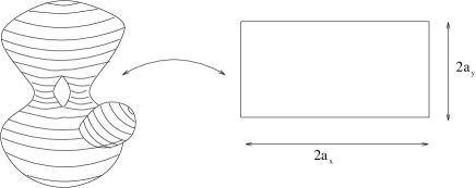
Figure 5.1: A torus made up of three sheets, may be mapped to a standard torus which is obtained by identifying opposite points on a rectangle.

Given the mapping, $z(u)$, one may now compute $S(z)$ using Eq. (5.1). $S(z)$ will have $n-1$ simple poles, outside the bubble, at points which we denote by $q_{i}$. Sufficiently close to these poles $S(z)$ takes the form

$$S(z)\sim-\frac{\mu_{i}}{z-q_{i}},\,\,\,\,\,\,i=1,2\cdots n-1,$$ (5.2)

Thus $q_{i}$ and $\mu_{i}$, may be viewed as the Miwa variables’ locations and weights, respectively. In addition, the singular behavior near infinity is

$$S(z)\sim t^{\prime}_{1}+\frac{t-\sum_{i=1}^{n-1}\mu_{i}}{z}.$$ (5.3)

By identifying the behavior near the singular points of Schwarz function from (5.1), and comparing this behavior with (5.2) and (5.3), one may construct a set of nonlinear equations which express the variables $t$, $t^{\prime}_{1}$ ,$\mu_{i}$ and $q_{i}$ in terms of parameters, $u_{i}$, $\alpha_{i}$, and $\beta$, of the map $z(u)$. The solution of these equations enables one to express the the conformal mapping parameters, $u_{i}$, $\alpha_{i}$, and $\beta$, as function of the time $t$, $t^{\prime}_{1}$ and the Miwa parameters.

Now, the Miwa variables, and $t^{\prime}_{1}$ are constants of motion. Thus keeping $q_{i}$, $\mu_{i}$ and $t^{\prime}_{1}$ fixed, and letting $t$ change, we obtain the time evolution of conformal mapping $z(u)$ which describes, in turn, the shape of the ST bubble as a function of the time.

To be more concrete, let us construct the nonlinear equations relating the conformal mapping parameters to the Miwa variables, and the times $t^{\prime}_{1}$ and $t$. Consider first the locations of the Miwa variables, $q_{i}$. Since $z(u)$ has a simple pole at $u_{i}$, where $1\leq i\leq n-1$, the Schwarz function $S(z)=\bar{z}(-u)$ would have poles at the images of $-\bar{u}_{i}$. These points are on the exterior of the bubble (due to the reflection property of $S(z)$ and since $u_{i}$, for $1\leq i\leq n-1$ have been chosen to be the pre-images of the “non-physical” infinities which can be viewed as located in the interior of the bubble) and should be identified with the location of the Miwa variables, Thus:

$$q_{i}=z(-\bar{u}_{i})\leavevmode\nobreak\ \leavevmode\nobreak\ \leavevmode\nobreak\ \mbox{for}\leavevmode\nobreak\ \leavevmode\nobreak\ \leavevmode\nobreak\ i=1,...n-1.$$ (5.4)

The weight of the Miwa variables, $\mu_{i}$, can be extracted by a local analysis of the behavior in the vicinity of the singularities. The result is

$$\mu_{i}=\left.\frac{\partial z}{\partial u}\right|_{-\bar{u}_{i}}\lim_{\delta u\rightarrow 0}\left(\bar{z}(\bar{u}_{i}+\delta u)\delta u\right).$$ (5.5)

Consider now the pole $u_{0}$ of $z(u)$ which is the pre-image of the physical infinity. As follows from (5.3), near the physical infinity, $S(z)\rightarrow t^{\prime}_{1}$, since also $S(z)=\bar{z}(-u)$, we conclude that

$$t^{\prime}_{1}=\bar{z}(-u_{0}).$$ (5.6)

A local analysis near the physical infinity allows one to extract the residue of the second term in (5.3). The result is

$$t-\sum_{i=1}^{n-1}\mu_{i}=-\left.\frac{\partial z}{\partial u}\right|_{-\bar{u}_{0}}\lim_{\delta u\rightarrow 0}\left(\bar{z}(\bar{u}_{0}+\delta u)\delta u\right).$$ (5.7)

The equations above, are the general equations of the Richardson approach.

5.2 One Miwa variable

We turn now to illustrate the approach outlined above for the case of 1-Miwa variable. We consider first the simplest case of a spectral surface of genus zero, comprised of two copies of the complex plain. As explained above the $u$-space is chosen to be the cylinder $-\infty<\Re(u)<\infty$ and $0\leq\Im(u)<2\pi$, where a period of $2\pi i$ is implied. The conformal mapping takes the form:

$$z(u)=\alpha_{0}\left(\frac{1}{e^{u-u_{0}}-1}-\frac{1}{e^{u-u_{1}}-1}\right)+\beta,$$ (5.8)

where $\alpha_{0}$, $u_{0}$, $u_{1}$ and $\beta$, are the conformal mapping parameters whose time dependence is to be determined. Notice that the above form of $z(u)$ is indeed correctly defined on the cylinder, namely it is periodic in $u\rightarrow u+2\pi i$. We can use equations (5.4-5.7) to express $q_{1},$ $t^{\prime}_{1},$ $\mu_{1},$ and $t$ in terms the conformal mapping parameters. The equations take the form:

$$q_{1}=\alpha_{0}\left(\frac{1}{e^{-\bar{u}_{1}-u_{0}}-1}-\frac{1}{e^{-\bar{u}_{1}-u_{1}}-1}\right)+\beta$$

$$t^{\prime}_{1}=\bar{\alpha}_{0}\left(\frac{1}{e^{-u_{0}-\bar{u}_{0}}-1}-\frac{1}{e^{-u_{0}-\bar{u}_{1}}-1}\right)+\bar{\beta}$$

$$\mu_{1}=-|\alpha_{0}|^{2}\left(\frac{e^{-u_{1}}}{\left(e^{-\bar{u}_{1}-u_{1}}-1\right)^{2}}-\frac{e^{-u_{0}}}{\left(e^{-\bar{u}_{1}-u_{0}}-1\right)^{2}}\right)$$

$$t-\mu_{1}=-|\alpha_{0}|^{2}\left(\frac{e^{-u_{1}}}{\left(e^{-\bar{u}_{0}-u_{1}}-1\right)^{2}}-\frac{e^{-u_{0}}}{\left(e^{-\bar{u}_{0}-u_{0}}-1\right)^{2}}\right)$$

Thus we have 4 unknowns and 4 equations. Solving these equations for the parameters of the mapping in terms of $\mu_{1}$, $q_{1}$, $t^{\prime}_{1}$ (which are constants) and the time $t$, gives the evolution of the conformal mapping (5.8) as function of the time. The contour of the bubble, ${\mathcal{C}}$ is the image of the line $\bar{u}=-u$ which in our case is $\Re(u)=0$, i.e.

$${\mathcal{C}}=\left\{z\right|\left.z=z(u),\Re(u)=0\right\}$$

The evolution of the contour $\mathcal{C}$ is demonstrated in Fig. 5.2. At some time $t^{*}$ the contour reaches a cusp beyond which the equations do not possess a physical solution.

Figure 5.2: Evolution of a 1-Miwa contour..

We turn now to consider the one-Miwa problem on genus-1 surface. Here we take $u$ space to be a torus realized as the rectangle. $-a_{x}\leq\Re(u)\leq a_{x}$ and $-a_{y}\leq\Im(u)\leq a_{y}$ with the usual identification of opposite sides. Provided that we choose the ratio $\frac{{a_{y}}}{{a_{x}}}$ correctly we may find a isomorphism between the rectangle and the spectral surface. In the one Miwa case such a mapping is provided by:

$$z(u)=\alpha_{0}\left(\zeta(u-u_{0})-\zeta(u-u_{1})\right)+\beta,$$ (5.9)

where $\alpha_{0}$, $u_{0}$, $u_{1}$ and $\beta$ are the parameters of the mapping and $\zeta$ is the Weierstrass zeta function, which is quasi-periodic with quasi-periods $2a_{x}$ and $2ia_{y}$:

$$\zeta(u+2a_{x})=\zeta(u)+2\eta_{x}$$

$$\zeta(u+2a_{y})=\zeta(u)+2\eta_{y}$$

Thus $z(u)$ is also doubly periodic as it must be in order for it to be defined on the rectangle with the opposite sides identified.

Equations (5.4-5.7) can be written explicitly as in the genus zero case, and their solutions yields the time dependence of the parameters of the conformal mapping (5.9). The evolution of the bubble contour can now be computed as the image of $\bar{u}=-u$.

However, in the genus-1 case, $\bar{u}=-u$ defines two contours.

$$\Re(u)=0,\,\,\mbox{ and}\,\,\,\Re(u)=a_{x}.$$

The first solution is already familiar from the genus-0 case it is the imaginary axis in $u$ plane which is mapped to the perimeter of the first bubble. The second solution, $\Re(u)=a_{x}$ follows from the torus topology where the line $\Re(u)=a_{x}$ is identified with the line $\Re(u)=-a_{x}$. Consequently, we arrive at the conclusion that one contour, ${\mathcal{C}}_{1}$, is the image of $\Re(u)=0,$ while the other contour, ${\mathcal{C}}_{2}$ is the image of $\Re(u)=a_{x}$:

$${\mathcal{C}}_{1}=\left\{z\right|\left.z=z(u),\Re(u)=0\right\}\leavevmode\nobreak\ \leavevmode\nobreak\ \leavevmode\nobreak\ \leavevmode\nobreak\ \leavevmode\nobreak\ \leavevmode\nobreak\ {\mathcal{C}}_{2}=\left\{z\right|\left.z=z(u),\Re(u)=a_{x}\right\}$$

We still have arbitrariness as for the choice whether the domain $0<\Re(u)<a_{x}$ will be considered the exterior of the domain or the interior. The choice must be made in such a way that the solution becomes physical, if possible. In the 1-Miwa case the genus-1 solutions are never physical, a point on which we will elaborate below.

5.3 Virtual bubbles

We turn now to explain why the genus-1 solution found for the 1-Miwa case are non physical. As we will show this non physicality may be understood as a situation where one of the bubble is of negative area. We refer to such bubbles as virtual bubbles, and show that if follows from the fact that the two closed contours described by $S(z)=\bar{z}$ are located on a different sheets of the Riemann surface.

If the two contours, ${\mathcal{C}}_{1}$ and ${\mathcal{C}}_{2}$ would lie on the same sheet then we would refer to this sheet as the physical plane, and consider the other sheets only as mathematical surfaces on which we extend the definition of $S(z)$. This would also determine the choice of domain on the rectangle that would represent the exterior of the bubbles - we would choose this domain as to contain the infinity which is on the same sheet as both the bubbles. This domain, which is on the exterior of the bubbles, naturally does not contain any branch points of the Schwarz function. To see that indeed the solutions that we have obtained are non-physical, we show that no matter which of the two possible domains we choose, we would have branch points of the Schwarz function in it. This is seen by the symmetry of $z(u):$

$$z\left(\frac{u_{0}+u_{1}}{2}+u\right)=z\left(\frac{u_{0}+u_{1}}{2}-u\right),$$

which follows from the anti-symmetry properties of the Weierstrass $\zeta$ function $\zeta(-u)=-\zeta(u)$. The four fixed points of this symmetry on the torus are the branch cuts (where the mapping $z(u)$ is not conformal, hence $z^{\prime}(u)=0$), these are the points:

$$u_{c},u_{c}+ia_{y},u_{c}+a_{x},u_{c}+a_{x}+ia_{y},$$

where $u_{c}=\frac{u_{0}+u_{1}}{2}$. The consequence of the fact that these are the branch points is that it does not matter whether we choose $0\leq\Re(u)\leq a_{x}$ as the exterior of the bubble or its complement, there will always be a branch point on the exterior of the bubble. This is not consistent with two physical bubbles, where one has the branch cuts inside each one of the bubbles. In fact in the genus-1 1-Miwa case, one must pass through the branch cut in order to get from the physical sheet to a point on the unphysical bubble. This is demonstrated in Fig. 5.3. In the fermionic picture (see Fig. 5.4) we may interpret the in-existence of physical solutions for the 1-Miwa case by the fact that there are no minima of the potential in which another bubble may form (there is one minimum which is occupied by the original bubble).

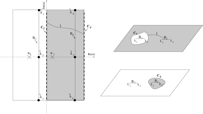
Figure 5.3: Schematic drawing of torus to the left and the two-sheeted Riemann surface to the right. Points $u_{0}$ and $u_{1}$ on the torus are mapped to the infinities on the upper and lower sheets respectively, while $\tilde{\lambda_{i}}$ are mapped to the branch points, $\lambda_{i}$. The branch cuts are $B_{i}$ drawn on the two sheeted Riemann surface as well as on the torus. The two contours are $C_{1}$ and $C_{2}$. A line connecting $C_{1}$ and $C_{2}$ ($l$ for example) must cross one of the branch cuts, which implies that the two contours lie on different sheets of the Riemann surface.

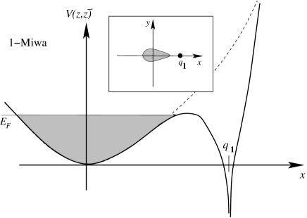
Figure 5.4: Schematic drawing of a Fermi sea filling up the 1-Miwa potential. The dotted line shows the potential with no Miwa variable. The Miwa variable introduces an infinite well at point $q_{1}$ (the location of the Miwa variable). The inset shows the shape of the droplet in this case. The cusps forms when the Fermi sea reaches a saddle point of the potential.

Chapter 6 Multi-bubble solutions

In the previous section we have solved the 1-Miwa case and demonstrated that the generalization to the genus-1 solutions does not solve the problem of going beyond the cusp since it generates non-physical solutions associated with virtual bubbles. Employing the noninteracting fermions picture we saw that this behavior signals the breakdown of the ST description of the problem.

We may resolve this problem by introducing an additional weak Miwa variable with negative weight which generate a local minimum of the potential near the cusp, as illustrated in Fig. (6.1). Thus as we increase the Fermi level, at some point, fermions will tunnel to the other minimum of the potential, and an additional droplet will form. In this situation we expect the additional droplet to be physical, see illustration in Fig. 6.1

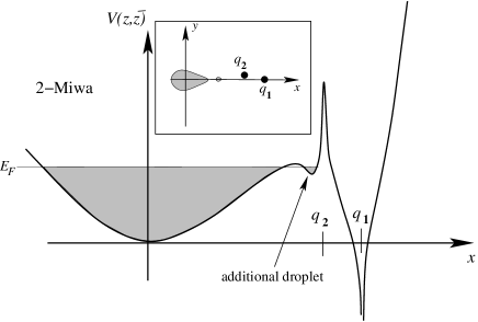
Figure 6.1: Schematic drawing of Fermi sea filling up the two-Miwa potential. an additional droplet now forms at the second minimum of the potential. The cusp that would have formed near the saddle between the two minima is regularized by this droplet. $q_{1}$ is the Miwa pole while $q_{2}$ is the Miwa zero.

In this section we shall present the solution of the 2-Miwa variable problem. Namely, we look for the solution of the problem whose Schwarz function on the exterior of the bubble has the singular structure:

$$S(z)\sim\frac{t-\mu_{1}+\mu_{2}}{z}+t^{\prime}_{1}-\frac{\mu_{1}}{z-q_{1}}+\frac{\mu_{2}}{z-q_{2}}$$

Following the Richardson approach one can solve this problem. In what follows we describe this solution.

By counting the number of points for which $z^{\prime}(u)=0$, one sees that there are $3$ branch cuts in this case. The number of copies of the complex plane of which the spectral surface is composed is $3$ (this can be seen from the fact that $z(u)$ diverges at three different points on the torus, which correspond to infinities on each one of the copies of the complex plane). This is consistent with the Riemann-Hurwitz formula which relates the number of branch points, $B$, the number of sheets, $n$, and genus $g$ of the Riemann surface:

$$g=1+\frac{B}{2}-n.$$

The difficulty which is introduced by taking a $3$-sheeted genus-1 Riemann surface is that it is not straightforward to write down the holomorphic differentials in this case. Thus using the Krichever equations to solve the evolution is more difficult .

Early stages: genus-0 solution

The early stages of the evolution, in the noninteracting fermion picture, can be associated with the situation were the Fermi energy is sufficiently low, such that the additional minimum of the potential is left unoccupied. This means that a mapping $u(z)$ is from the cylinder $-\infty<r<\infty$, $0\leq\theta<2\pi$ to a genus-0 surface composed of 3 copies of the complex plain (1 plus the number of Miwa variables), as illustrated in Fig. (6.2).

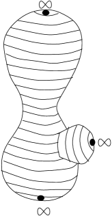
Figure 6.2: The Riemann surface of genus-0 2-Miwa aggregate. The Riemann surface is composed of three sheets (the points at infinity on each of the sheets are shown). The third sheet is schematically shown on the graph as an additional surface tacked on the Riemann sphere.

Thus the mapping, $z(u)$, from the cylinder to the spectral surface is given by:

$$z(u)=\frac{\alpha_{0}}{e^{u-u_{0}}-1}+\frac{\alpha_{1}}{e^{u-u_{1}}-1}-\frac{\alpha_{0}+\alpha_{1}}{e^{u-u_{2}}-1}+\beta$$

where $\alpha_{i}$, $u_{i}$ and $\beta$ are parameters whose time evolution is to be determined. The extraction of this time dependence using Richardson’s approach, shows that the bubble develops a cusp as in the one-Miwa case. This cusp, in the noninteracting fermion picture, appears when the Fermi level reaches the local maximum of the potential, see Fig. (5.4).

Mid-stage: genus-1 solution

The lesson from the Gurevich-Pitaevskii scenario, is that at some point, before the cusp, we must allow for a topological transition to take place, i.e. let the genus-1 solution take over, by forming an additional bubble. In the noninteracting fermion picture it is the time where the Fermi level reaches the local minimum of the potential. A smooth transition between the two solutions can happen only if the area of the second bubble vanishes in the genus-1 solution.

The mapping during this time is from the torus to the spectral surface of genus-1 topology

$$z(u)=\alpha_{0}\zeta(u-u_{0})+\alpha_{1}\zeta(u-u_{1})-(\alpha_{0}+\alpha_{1})\zeta(u-u_{2})+\beta.$$

where as before the evolution of the contour can be found by applying the Richardson approach to extract the time dependence of the coefficients $\alpha_{i}$, $u_{i}$ and $\beta$, keeping the normalization

$$\Re\left(\oint S(z)dz\right)=0,$$

for every cycle on the Riemann surface, where $S(z)=\bar{z}(-u(z))$. Details of this calculation can be found in Appendix E

Late stage: genus-0 solution

Increasing further the time causes another topological transition to take place. This time one switches from a genus-1 solution back to a genus-0 solution (in analogy to the GP scenario in KdV). The reason for this transition is the merging of the two bubbles as the Fermi surface becomes higher than the sadle points between the two minima of the potential. The two bubbles merge through a cusp, a treatment of the shape of the cusp is given in Appendix F.

Chapter 7 Tip-splitting

In this chapter we focus our attention on the tip-splitting shape which is formed after dispersive regularization of the cusp. We are lead to study tip-splitting since one expects that an understanding of the global structure of the ST bubble can be deduced from properties of the basic elements of the growing process, such as tip-splitting and side-branching. Indeed, studies of theoretical models of diffusion limited aggregation[13], and their generalizations (e.g. the dielectric breakdown model) demonstrate that the fractal dimension of the corresponding patterns is related to characteristics of the tip-splitting events[56] (side-branching in these models is negligible). The central result of this chapter is a formula which describes the evolution of tip splitting in time:

$$\frac{z(s,t)}{L}=s+u_{\phi}(t)+\frac{v_{\phi}(t)}{w_{\phi}(t)\pm\sqrt{s}}.$$ (7.1)

Here $z=x+iy$ is a complex coordinate, $L$ is the scale of the tip-split, $s>0$ parametrizes the curve, and $u_{\phi}(t)$, $v_{\phi}(t)$ and $w_{\phi}(t)$ are functions of the time, $t$. These functions which will be calculated in what follows, depend on a single parameter, $\phi$, governing the asymmetric shape of the evolution. In Fig. 7.1 we depict contours obtained from (7.1) which represent snapshots of the tip-splitting evolution as function of the time.

Figure 7.1: The evolution of tip splittings in the Saffman-Taylor problem at zero surface tension. The contours represent snapshots of the evolution as function of the time. The evolution given in (7.1), is characterized by one parameter, $\phi$, which controls the asymmetry between the two generated fingers. Panel A shows the symmetric evolution, while panel B represents a typical asymmetric behavior.

To begin with, it is important first to clarify what precisely we mean by a “tip”. In the ST problem with zero surface tension there is a natural way to define a tip. The reason is that in this case, for almost any initial bubble shape, fingers develop into cusps (see, e.g., panels A and B in Fig. 7.1). Here we focus our study at the solution of the ST problem well after the merging took place, at the period of the tip-splitting scenario illustrated in Fig. 7.1. We use the 2-Miwa potential introduced in Chapter 6, to obtain such a tip-splitting solution.

For actual calculation of the contour’s evolution it will be convenient to use a conformal mapping which maps the exterior of some “source domain” (in $\zeta$-plane) to the exterior of the physical bubble, the “target domain” (in $z$-space). The source domain is usually taken to be the unit circle, however, we found it more convenient to use a bubble with a cusp. The advantage in using this source domain is that we can choose the mapping to be non-trivial only around the tip, while everywhere else it would be approximately proportional to the identity map.

We will study the evolution near the tip in the case where the weight of one of the Miwa variables, is small compared to the other. This suggests choosing the source domain to be the one Miwa-variable bubble at the point where a cusp is formed. The Riemann surface in this case is composed of two sheets as described above. If we assume this surface to be of genus zero, then by the Riemann-Hurwitz theorem, the number of branch points is two. Thus the Riemann surface is given by the polynomial equation $R^{2}=(\zeta-\lambda_{1})(\zeta-\lambda_{2})$. A function defined on this surface (the Schwarz function in particular) contains a branch cut which extends from point $\lambda_{1}$ to the point $\lambda_{2}$. An example of such a function is $R(\zeta)$.

The 1-Miwa bubble is characterized by four parameters $t_{1},t,q$ and $\mu$, since the location of the branch points depends on these parameters, one can calculate the area of the bubble and its first harmonic moment, $t_{1}$, from the location of the branch points $\lambda_{1}$ and $\lambda_{2}.$ We will fix $\mu=-q=1$ and treat $\lambda_{1}$ and $\lambda_{2}$ as the parameters which describe the bubble. If we also demand that the bubble is at the moment where the cusp forms, we can characterize the bubble by a single parameter, say $\lambda_{1}$. We assume that $\lambda_{1}<\lambda_{2}$ and that $\lambda_{1}$ is of order $\delta,$ where $\delta\ll 1$. This assumption implies that the global bubble shape is dominated by the cusp. Then the bubble area is of order $\delta^{3}$ while the first harmonic moment, $t_{1},$ is $1+O(\delta^{2})$. The Schwarz function, $\sigma(\zeta)$, of such a bubble is:

$$2\sigma(\zeta)=\left(t_{1}-1\right)+\frac{t-1}{\zeta-\bar{t}_{1}}-\frac{1}{\zeta+1}+\frac{(t_{1}+1)(\zeta-\lambda_{1})R(\zeta)}{(\zeta-t_{1})(\zeta+1)},$$

as can be ascertained by examining this function’s singular structure and that it satisfies the unitarity condition (2.6). The fact that this function describes a bubble with a cusp can be checked by considering the behavior of the solution of $\sigma(\zeta)=\bar{\zeta}$ near $\lambda_{1}$ (where the cusp is located).

Up till now we have characterized the “source domain”. We would like, now, to specify the physical bubble, or the “target domain” associated with two Miwa variables. For this purpose we must give the mapping between the source and target domains. This mapping is taken to be:

$$z(\zeta)=c_{1}\left(\zeta+\frac{\alpha}{2}\frac{R(\theta)-R(\zeta)}{\zeta-\theta}+\beta R(\zeta)\right)+c_{2},$$ (7.2)

where $c_{1}$, $c_{2}$, $\alpha$, $\beta$, and $\theta$ are parameters of the mapping and $R(\zeta)\equiv\sqrt{\zeta-\lambda_{1}}\sqrt{\zeta-\lambda_{2}}$. This mapping can be considered as a mapping from the 1-Miwa Riemann surface to the 2-Miwa Riemann surface. The mapping has singularities at the infinities on each of the sheets of the Riemann surface associated with the source domain, which are mapped to infinities on different sheets on the target domain, as well as at the point $\theta$ on the unphysical sheet. This point, $\theta,$ is mapped to an infinity on a third sheet of the target Riemann surface. Thus (7.2) indeed maps a two-sheeted Riemann surface, which is associated with a 1-Miwa bubble, to a three sheeted Riemann surface.

That, indeed, the target Riemann surface is associated with a 2-Miwa variable bubble, can be deduced from the singular structure of the Schwarz function of the target domain. The latter is given by $S(z)=\bar{z}\left(\sigma\left(\zeta\left(z\right)\right)\right)$, where $\zeta(z)$ is the inverse map of $z(\zeta)$, and $\sigma(\zeta)$ is the Schwarz function of the source domain.

Having $S(z)$ one may extract all constants of motion (Miwa variables, $q_{1}$, and $q_{2}$; Miwa weights, $\mu_{1}$ and $\mu_{2}$; and $t_{1}$), and the area $t$, from its singular structure. These will be expressed as functions of the parameters of the mapping (7.2) and $\lambda_{1}$. Solving these relations one may express the parameters of the mapping as functions of the time and thus obtain the evolution of the contour. We take $\mu_{1}=-q_{1}=1$ by fixing $c_{1}$ and $c_{2}$. Thus the parameters whose time evolution is to be determined are $\alpha$, $\beta$, $\theta$ and $\lambda_{1}$.

To obtain reasonably simple equations, we expand all quantities in orders of $\delta$ and take the leading order. Let us assume that for some initial moment, $t^{(0)}$, around the formation of the tip, $\lambda_{1}$ assumes the value $\lambda$, to leading order in $\delta$. We now make the following scaling ansatz: $\alpha\sim\delta^{4}$, $\beta\sim\delta^{3}$, $\nu\equiv\lambda_{1}-\theta\sim\delta^{3}$ and $\delta\lambda\equiv\lambda_{1}-\lambda\sim\delta^{3}$. Then the equations we obtain, to leading order in $\delta$, for the constants of motion $q_{2}-\lambda$ and $\mu_{2}$ are:

$$q_{2}-\lambda=\beta+\delta\lambda-\bar{\nu}-\frac{\alpha\sqrt{-\lambda}}{\sqrt{\nu}+\sqrt{\bar{\nu}}}\leavevmode\nobreak\ \leavevmode\nobreak\ \leavevmode\nobreak\ \leavevmode\nobreak\ \leavevmode\nobreak\ \leavevmode\nobreak\ \leavevmode\nobreak\$$ (7.3)

$$\mu_{2}=-2\bar{\alpha}\sqrt{-\lambda}\sqrt{\nu}\left(1-\frac{\alpha\sqrt{-\lambda}}{2\sqrt{\bar{\nu}}\left(\sqrt{\nu}+\sqrt{\bar{\nu}}\right)}\right)$$ (7.4)

Let us now define $T_{1}=t_{1}-\left(1+3\lambda^{2}-7\lambda^{3}+\frac{33}{2}\lambda^{4}\right)$ (the difference between the first harmonic moment of the target bubble and a source bubble with $\lambda_{1}=\lambda$ to order $O(\delta^{5})$), and similarly $T=t-(-4\lambda^{3}+18\lambda^{4}-63\lambda^{5})$. With these definitions, analysis of the singularities of $S(z)$ yields:

$$T=2\Re(\alpha)\lambda+4\beta\lambda^{2}-12\lambda^{2}\delta\lambda,$$ (7.5)

$$T_{1}=\Re(\alpha)-2\beta\lambda+6\lambda\delta\lambda.$$ (7.6)

The solution of Eqs. (7.3-7.6) give the parameters $\alpha,$ $\beta,$ $\nu$ and $\delta\lambda$ in terms of $q_{2},$ $\mu_{2}$, $T$ and $T_{1}$, which define, in turn, the conformal mapping of the contour on the target space as function of the time. To write down the solution of these equations it will be convenient to define a shifted rescaled time $\delta t\equiv-\frac{T+2T_{1}\lambda}{4\mu_{2}^{3/4}\sqrt{-\lambda}}$ and introduce two functions $\xi$ and $\eta$ which satisfy the nonlinear equations:

$$\left(\frac{\sqrt{2}\delta t}{\sqrt{\xi}}+\frac{\delta t^{2}}{2\xi^{2}}\right)\left(\eta+\xi\right)=1;\leavevmode\nobreak\ \leavevmode\nobreak\ \eta=\left(\frac{\phi}{\sqrt{\xi}-\frac{\delta t}{\sqrt{2}\xi}}\right)^{2},$$

where $\phi=\Im\left(\frac{q_{2}}{\sqrt{\mu_{2}}}\right)$ is the asymmetry parameter. The solution of these equations gives $\eta$ and $\xi$ as functions of the rescaled time, $\delta t$, and $\phi$. With the help of these functions we may write the solution of Eqs. (7.3-7.6) as:

$$\alpha=\frac{\mu_{2}^{3/4}\delta t}{\sqrt{-\lambda}}\left(-1+i\sqrt{\frac{\eta}{\xi}}\right),\leavevmode\nobreak\ \leavevmode\nobreak\ \leavevmode\nobreak\ \leavevmode\nobreak\ \leavevmode\nobreak\ \leavevmode\nobreak\ \leavevmode\nobreak\ \leavevmode\nobreak\ \leavevmode\nobreak\ \leavevmode\nobreak\ \leavevmode\nobreak\ \leavevmode\nobreak\ \leavevmode\nobreak\ \leavevmode\nobreak\ \leavevmode\nobreak\ \leavevmode\nobreak\ \leavevmode\nobreak\ \leavevmode\nobreak\ \leavevmode\nobreak\ \leavevmode\nobreak\ \leavevmode\nobreak\ \leavevmode\nobreak\ \leavevmode\nobreak\ \leavevmode\nobreak\ \leavevmode\nobreak\ \leavevmode\nobreak\ \leavevmode\nobreak\ \leavevmode\nobreak\ \leavevmode\nobreak\$$

$$4\beta=3\Re(q_{2})-3\lambda-\frac{3}{2}(\eta-\xi)-\frac{3\delta t}{\sqrt{2\xi}}-\frac{T_{1}}{4\lambda}+\frac{T}{8\lambda^{2}},$$

$$\nu=\frac{\xi-\eta}{2}+i\sqrt{\xi\eta},\leavevmode\nobreak\ \leavevmode\nobreak\ \leavevmode\nobreak\ \leavevmode\nobreak\ \leavevmode\nobreak\ \leavevmode\nobreak\ \leavevmode\nobreak\ \leavevmode\nobreak\ \leavevmode\nobreak\ \leavevmode\nobreak\ \leavevmode\nobreak\ \leavevmode\nobreak\ \leavevmode\nobreak\ \leavevmode\nobreak\ \leavevmode\nobreak\ \leavevmode\nobreak\ \leavevmode\nobreak\ \leavevmode\nobreak\ \leavevmode\nobreak\ \leavevmode\nobreak\ \leavevmode\nobreak\ \leavevmode\nobreak\ \leavevmode\nobreak\ \leavevmode\nobreak\ \leavevmode\nobreak\ \leavevmode\nobreak\ \leavevmode\nobreak\ \leavevmode\nobreak\ \leavevmode\nobreak\ \leavevmode\nobreak\ \leavevmode\nobreak\ \leavevmode\nobreak\ \leavevmode\nobreak\ \leavevmode\nobreak\ \leavevmode\nobreak\ \leavevmode\nobreak\ \leavevmode\nobreak\ \leavevmode\nobreak\ \leavevmode\nobreak\ \leavevmode\nobreak\$$

$$4\delta\lambda=3\Re(q_{2})-3\lambda-\frac{3}{2}(\eta-\xi)-\frac{3\delta t}{\sqrt{2\xi}}+\frac{T_{1}}{4\lambda}-\frac{T}{8\lambda^{2}}.$$

Given this time dependence of the parameters of the conformal mapping we are in a position to describe the contour dynamics in the vicinity of the tip-splitting. For this purpose it is sufficient to focus on the image of the source domain around the cusp. The shape of the source domain near the cusp is given by the universal form $y=A\delta x^{3/2}$, were $\delta x\equiv x-\lambda_{1}$, and $A$ is some constant. Close enough to the cusp $y\ll\delta x,$ and therefore we may assume that $y\simeq 0$ (this assumption can be proved to be consistent with the $\delta$ expansion performed here). Thus one has to find the image of the ray $x>\lambda_{1}$ under the mapping $z(\zeta)$ to leading order in $\delta$. The result is given by Eq. (7.1), where $L=\sqrt{\mu_{2}}$ and the functions $u_{\phi}(t)$, $v_{\phi}(t)$, and $w_{\phi}(t)$ are:

$$u_{\phi}(t)=\frac{\xi-\eta}{2}-\frac{\delta t}{\sqrt{2\xi}},$$

$$v_{\phi}(t)=\delta t\left(1-i\sqrt{\frac{\eta}{\xi}}\right),$$

$$w_{\phi}(t)=\frac{\xi-\eta}{2}+i\sqrt{\eta\xi}.$$

The above equations together with (7.1) describe the evolution of a tip-splitting of the ST problem at zero surface tension (Fig. 1). The form of the tip-splitting depends on a single parameter, $\phi$, which controls the asymmetric shape of the evolution. Since our derivation of the tip-splitting formula makes use only of local properties near the tip, it is suggestive that this evolution is universal. Namely, the tip splitting evolution is characterized by one parameter, $\phi$, independent of the shape of the bubble on large scales. The shortcomings of our result is that it does not include the influence of surface tension. Therefore it breaks down after a short time due to the formation of cusps. The procedure of dispersive regularization must be repeated again and again in order to obtain large aggregates.

7.1 Tip-Splitting Scaling and Fractal Dimension

As noted above, tip-splitting is believed to be important in the understanding of the fractal properties of the ST aggregate. Indeed, Halsey has argued that the DLA may be viewed as repeated tip splitting events which give rise the branched growth of the fractal[56]. This prompts us to study the tip-splitting we have obtained in this light. In particular, we want to understand what are the scaling properties of the tip splitting solution. In order to do this, we first note that the length scale of the tip-split, namely $L\equiv\sqrt{\mu_{2}}$ scales as $\delta^{3}$ while the shifted time, $T$, scales as $\delta^{5}$. This suggests that the shape of the tip split would depend on time through the parameter $\frac{\tau}{L^{5/3}}$, where $\tau\equiv T+2T_{1}\lambda$. Indeed, the parametric form of the tip split shape (7.1) may be rewritten as:

$$\left(\begin{array}[]{c}x(t,s)\\ y(t,s)\end{array}\right)=L\vec{f}\left(s,\frac{\tau}{L^{5/3}}E,\phi\right),$$ (7.7)

where $E=\sqrt{-\frac{\mu_{2}^{1/6}}{\lambda}}$ does not scale with $\delta$ as can be straightforwardly checked. We will assume that parameters which do not scale with $\delta$ depend only on the large scale structure of the bubble. $E$ may be interpreted as a parameter which determines the fraction of the area which is added to the vicinity of the tip split. $E$ will be effected by how much the large scale structure of the bubble screens the tip-split area, and on how much the tip-split protrudes from the bubble. Equation (7.7) suggests that the lengths scale as $\tau^{3/5}.$ In DLA clusters, the linear size of the aggregate scales with the number of particles as $t^{\frac{1}{D}},$ where $D=1.71,$ is the fractal dimension of the aggregate.

We come to the conclusion that from the naive scaling argument, the fractal dimension of the bubble would be $5/3=1.66\ldots,$ close to the measured fractal dimension of the DLA aggregate. However, the linear size which appears in equation (7.7), $L$, is the size of a single tip split, while in the fractal, it is the overall size of the cluster that would scale as $t^{\frac{1}{D}}$. Thus in order to relate the scaling of a single tip-split to that of the fractal we have to assume that many small tip-split events may be coarse grained into a large one. Then if we assume self-similarity, the relation between the time $\tau$ and the size $L$ would be retained, also for tip-splits whose size is of the order of the whole aggregate. In particular, the radius of the bubble which is of order of the strongest branch would scale as $t^{3/5}$, where $t$ is the area of the droplet. Thus we would obtain $5/3$ for the fractal dimension of the aggregate. Apart from the assumption of self-similarity, to obtain this result we have also assumed that the parameters $E$ and $\phi$ do not change in the renormalization process, as they do not scale with $\delta$. A more rigorous treatment, which relaxes this “mean filed” assumption may take into account different effects neglected here, in a way that would produce a more accurate estimate of the fractal dimension.

Chapter 8 Discussion

In this thesis we made use of the relation between the quantum Hall effect, the integrable hierarchy of the 2DTL, and the idealized ST problem in order to describe its dynamics. For this purpose we have used the dispersive regularization method of soliton theory. This method, in essence, is an extension of the Whitham equations to spectral surfaces of non-trivial topology (nonzero genus). This approach amounts to the generalization of the idealized ST problem to the multi-bubble case. The bubbles share the same pressure, and their evolution is dictated by the requirement that the harmonic moments are fixed, and the total area of the bubbles is proportional to the time.

In the picture of noninteracting fermions, this regularization has a simple interpretation: Consider a potential with multiple minima, and let us fill the potential with fermions injected adiabatically at the lowest minimum of the potential. We may consider now two procedures of taking the semi-classical limit. In the first one $\hbar\rightarrow 0$ and then time is sent to infinity (notice that here time has nothing to do with the area of the droplet which is determined by the number of fermions). In this case the fermions cannot tunnel into other minima, and once the filling is such that the fermion droplets reaches the saddle point, the dynamics cannot be continued adiabatically any longer. In the second limiting procedure, we first take time to infinity and only then $\hbar\rightarrow 0$, with this order of limits, tunneling is allowed at any step, and fermions may form multiple droplets. These multiple droplets are the multi-bubble solutions of the idealized ST problem.

As we show, in the multi-bubble solutions, situations may occur where bubbles of negative area are developed. One may try, in this case, to focus on the dynamics of only the physical bubbles. However, this viewpoint implies that pressure in the exterior domain is not harmonic and that the harmonic moment of the physical bubbles are, in general, not conserved. Therefore virtual bubble solutions do not represent a clear regularization of the ST evolution, and their physical meaning is still obscure.

Nevertheless, one may choose a set of initial conditions in which the integral representation of the $\tau$-function converge. In this case, all bubbles which may appear are real (have positive area). The dynamics of this generalized system may be viewed as a situation in which pumping of the non-viscous fluid is done simultaneously into more than one point of the Hele Show cell, as illustrated in Fig. 8.1.

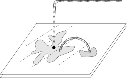
Figure 8.1: Multi-bubble dynamics realized as an ST problem in which the non-viscous fluid is injected at more than one point into the Hele-Shaw cell.

The main problem is to what extent this type of solutions may be viewed as regularization of the idealized ST problem. An evolution where new bubbles appear and merge with the original bubble is clearly not equivalent to the evolution of the ST problem with finite small surface tension, since in the latter only one bubble exist. Nevertheless, one may hope that the global structure of both problems is statistically the same, analogous to the arguable equivalence between some statistical features (e.g., the fractal dimension) of diffusion limited aggregation (DLA) and the ST with small surface tension. If this is indeed, the situation, then one may regard the multi-bubble model as an integrable regularization of the ST problem. This model can be viewed as a hybridization of DLA and the idealized ST dynamics, since the new bubbles which appear near the tips of the fingers may be regarded as DLA particles sticking to the aggregate.

Yet, one can easily imagine simple examples where the multi-bubble solutions clearly cannot be considered as a regularization. For instance, the merging of two big bubbles, or situations where bubbles engulf large droplets of viscous fluid. To avoid these situations one must find a method which eliminates these cases, but nevertheless, allows one to choose a generic initial condition. Such a method would amount to finding appropriate potentials, or sets of harmonic moments $\{t_{k},\bar{t}_{k}\}$ such that the small droplets would have some characteristic length scale. A different approach would be to start from a well developed DLA or ST bubble and take the inverse time evolution, which is dispersively regularized. A weak condition for the dispersively regularized evolution to be in the same class as the DLA or ST evolution would be that the aggregate retains its fractal dimension as its area is decreased.

A different route is to focus on the local properties of the ST singularities. This viewpoint is motivated by studies of DLA and its generalization, the dielectric breakdown model, which demonstrate that the fractal dimension of the corresponding patterns is related to properties of individual tip-splitting events (side-branching in these models is negligible). Indeed, tip splitting appears, generically, after the merging of two bubbles (see panel E. in Fig. 4.1), and their form is believed to be universal. We studied the tip-splitting which appears in the two-Miwa case and saw that its scaling properties is congruent, through a naive argument, with a fractal of dimension $5/3=1.66\ldots.$, while the measured fractal dimension of a DLA clusters is $1.71$. One thus may hope that by a more rigorous treatment, which nevertheless makes use of the ideas of the naive argument, would produce results closer to the measured fractal dimension.

Appendix A Proof of 2DTL for $\tau_{N}$

In this Appendix we will derive Eq. (3.7) showing that $\tau$-function satisfy the 2DTL equations, our treatment follows the one presented in Ref. [57], with the necessary modifications appropriate for a two-dimensional Coulomb gas. First, the normalization of the orthogonal polynomials is given by:

$$\int\overline{P_{n}(z)}e^{-|z|^{2}+\sum_{k}t_{k}z^{k}+c.c.}P_{m}(z)d^{2}z=e^{\phi_{n}}\delta_{nm}.$$

We shall use the fact that orthogonal polynomials are also orthogonal to any lower order polynomial:

$$k<N\Rightarrow\int\overline{P_{n}(z)}z^{k}e^{-|z|^{2}+\sum_{k}t_{k}z^{k}+c.c.}d^{2}z=0.$$

We wish now to find the equations that $\psi_{n}$ (given in equation (3.5)) satisfies. We define the infinite vector $\vec{\psi}(z)$ with elements $\psi_{n}(z).$ The functions $\psi_{n}(z)$ satisfy:

$$\int\overline{\psi_{n}(z)}\psi_{m}(z)=e^{\phi_{n}}\delta_{nm}.$$

We differentiate this relation with respect to $t_{1}$ and $\bar{t}_{1}$ and get:

$$\int\left(\frac{\partial}{\partial t_{1}}\overline{\psi_{n}(z)}\right)\psi_{m}(z)+\int\overline{\psi_{n}(z)}\left(\frac{\partial}{\partial t_{1}}\psi_{m}(z)\right)=\frac{\partial\phi_{n}}{\partial t_{1}}e^{\phi_{n}}\delta_{nm}$$ (A.1)

$$\int\left(\frac{\partial}{\partial\bar{t}_{1}}\overline{\psi_{n}(z)}\right)\psi_{m}(z)+\int\overline{\psi_{n}(z)}\left(\frac{\partial}{\partial\bar{t}_{1}}\psi_{m}(z)\right)=\frac{\partial\phi_{n}}{\partial\bar{t}_{1}}e^{\phi_{n}}\delta_{nm}$$ (A.2)

Note that differentiating $P_{n}(z)$ with respect to either $t_{1}$ or $\bar{t}_{1}$ we get a polynomial of degree $n-1$. Thus for example in

$$\frac{\partial}{\partial t_{1}}\psi_{m}(z)=\frac{\partial}{\partial t_{1}}P_{m}(z)e^{-\frac{|z|^{2}}{2}+\sum_{k}t_{k}z^{k}}=\left(\frac{\partial}{\partial t_{1}}P_{m}(z)\right)e^{-\frac{|z|^{2}}{2}+\sum_{k}t_{k}z^{k}}+z\cdot P_{m}(z)e^{-\frac{|z|^{2}}{2}+\sum_{k}t_{k}z^{k}}$$

only the second term on the RHS of the equation just above contributes to the integral $\int\overline{\psi_{n}(z)}\left(\frac{\partial}{\partial t_{1}}\psi_{m}(z)\right)$ when $n>m$. Thus for $n>m$ we have:

$$\int\overline{\psi_{n}(z)}\left(\frac{\partial}{\partial t_{1}}\psi_{m}(z)\right)=\int\overline{\psi_{n}(z)}z\psi_{m}(z)$$

Note that when $n>m,$ the expression on the RHS is non-zero only for $n=m+1.$ If we calculate the quantity $\int\overline{\psi_{n}(z)}\left(\frac{\partial}{\partial t_{1}}\psi_{m}(z)\right)$ for all $n$ we will be able to calculate $\frac{\partial}{\partial t_{1}}\psi_{m}(z)$ using a completeness relation. In order to do so we look at $\int\left(\frac{\partial}{\partial t_{1}}\overline{\psi_{n}(z)}\right)\psi_{m}(z)$ in equation (A.1). Using orthogonality we can again surmise that $\int\left(\frac{\partial}{\partial t_{1}}\overline{\psi_{n}(z)}\right)\psi_{m}(z)=0$ for $n\leq m.$ Now since the RHS of (A.1) is also zero for $n<m$ we come to the conclusion that $\int\overline{\psi_{n}(z)}\left(\frac{\partial}{\partial t_{1}}\psi_{m}(z)\right)=0$ for $n<m$. For $n=m$ the RHS in (A.1) gives $\frac{\partial\phi_{n}}{\partial t_{1}}e^{\phi_{n}}$ and so we have $\int\overline{\psi_{n}(z)}\left(\frac{\partial}{\partial t_{1}}\psi_{n}(z)\right)=\frac{\partial\phi_{n}}{\partial t_{1}}e^{\phi_{n}}.$ This is all the information we need in order to use the completeness relation:

$$\frac{\partial}{\partial t_{1}}\psi_{m}(z)=\sum_{n}\frac{1}{\int\overline{\psi_{n}(z)}\psi_{n}(z)}\psi_{n}(z)\int\overline{\psi_{n}(z)}\left(\frac{\partial}{\partial t_{1}}\psi_{m}(z)\right)=$$

$$=\sum_{n}e^{-\phi_{n}}\psi_{n}(z)\int\overline{\psi_{n}(z)}\left(\frac{\partial}{\partial t_{1}}\psi_{m}(z)\right)=\frac{\partial\phi_{m}}{\partial t_{1}}\psi_{m}(z)+e^{-\phi_{m+1}}\psi_{m+1}\int\overline{\psi_{m+1}(z)}z\psi_{m}(z)$$

The term $c_{0}\equiv e^{-\phi_{m+1}}\psi_{m+1}\int\overline{\psi_{m+1}(z)}z\psi_{m}(z)$ is recognized as the leading term in the expansion of $z\psi_{m}$ in terms of orthogonal polynomials, $z\psi_{m}=c_{0}\psi_{m+1}+c_{1}\psi_{m}+c_{2}\psi_{m-1}+...$ and since we normalize the orthogonal polynomials to have a unit leading coefficient we conclude that $c_{0}=1$. Thus

$$\frac{\partial}{\partial t_{1}}\psi_{m}(z)=\frac{\partial\phi_{m}}{\partial t_{1}}\psi_{m}(z)+\psi_{m+1}.$$

This equation can be written in the form:

$$\frac{\partial}{\partial t_{1}}\vec{\psi}=\left(e^{\partial_{t}}+\frac{\partial\phi_{t}}{\partial t_{1}}\right)\vec{\psi},$$

where $e^{\partial_{t}}$ is the shift operator with respect to the index of the vector $\psi$ (this index will be denoted by the letter $t$) Similar arguments lead us, through the use of (A.2) to the equation:

$$\frac{\partial}{\partial\bar{t}_{1}}\vec{\psi}=-e^{\phi_{n}-\phi_{n-1}}e^{-\partial_{t}}\vec{\psi}$$

Now consider the compatibility of these two equations:

$$\frac{\partial}{\partial\bar{t}_{1}}\frac{\partial}{\partial t_{1}}\vec{\psi}=\frac{\partial}{\partial t_{1}}\frac{\partial}{\partial\bar{t}_{1}}\vec{\psi}$$

This leads to:

$$\left[-\frac{\partial}{\partial t_{1}}+e^{\partial_{t}}+\frac{\partial\phi_{t}}{\partial t_{1}},\frac{\partial}{\partial\bar{t}_{1}}+e^{\phi_{n}-\phi_{n-1}}e^{-\partial_{t}}\right]=0$$

Which reduces to the following equations:

$$\frac{\partial^{2}}{\partial t_{1}\partial\bar{t}_{1}}\phi_{t}=e^{\phi_{t}-\phi_{t-1}}-e^{\phi_{t+1}-\phi_{t}}$$ (A.3)

Namely the 2-dimensional Toda lattice equations. Since $\tau_{N}=\Pi_{i=0}^{N}\tau_{i}$ this equation may be written as (3.7).

Appendix B The KdV equation

In this Appendix we outline the way in which the KdV equation can be integrated using the algebro-geometrical approach. The starting point is to represent the KdV equation (4.1) with $\beta=1$ in the Lax form [58]. For this we define the Lax operator, $L$:

$$L=-\partial_{x}^{2}-\frac{1}{6}u,$$

which is just the Schröedinger operator with a solution of the KdV equation inserted as a potential. We also define the operator, $A$:

$$A=4\partial_{x}^{3}+\frac{1}{2}\left(u\partial_{x}+\partial_{x}u\right).$$

One can now check, by direct substitution, that

$$\partial_{t}L=\left[A,L\right],$$ (B.1)

is equivalent to the KdV equation:

$$\partial_{t}u=u\partial_{x}u+\partial_{x}^{3}u.$$

Let us look for solutions of the spectral equation

$$L\psi=\lambda\psi,$$ (B.2)

whose time evolution is given by:

$$A\psi=\partial_{t}\psi.$$

These two equations are compatible by (B.1).

One may try to find different nonlinear integrable equations by choosing appropriate Lax pairs. Namely we should search for a differential anti-Hermitian operator $B_{n},$ $n\geq 0,$ such that:

$$\partial_{t_{n}}L=\left[B_{n},L\right].$$

The anti-Hermiticity of $B_{n}$ ensures that the spectrum of the operator $L$ does not depend on time. If we manage to have the RHS be a multiplicative operator (an operator which multiplies a function by another function), then we would have an equation of the form:

$$\partial_{t_{n}}u=F_{n}(u,\partial_{x}u,\partial_{x}^{2}u,...).$$

We have designated a different time, $t_{n},$ for evolutions generated by different operators $B_{n}$. We may now treat $u$ as a function of an infinite set of times,

$$u(t_{0},t_{1},t_{2},t_{3},...),$$

where $x$ corresponds to $t_{0}$ and $t$ stands for the time, $t_{1}.$ We already know $B_{0}$ and $B_{1}$:

$$B_{1}=A,\,\,\,\,\,B_{0}=\partial_{x}.$$

Higher $B$’s may be found by formally expanding $L^{\frac{2n+1}{2}}$, where $u$ is a small parameter, and retaining only the part which has positive powers in the derivative (designated by the ‘+’ subscript below). Thus, for example:

$$B_{1}=\left(-L\right)_{+}^{\frac{3}{2}}=\left[\partial_{x}^{3}+\frac{1}{4}\left(\partial_{x}u+u\partial_{x}\right)+O\left(\partial_{x}^{-1}\right)\right]_{+}.$$

See, e.g., [58] for more details. We can now choose the time evolution of the wave function to be consistent with the generators associated with the infinite set of times:

$$\partial_{t_{n}}\psi=B_{n}\psi.$$ (B.3)

The wave function $\psi$ depends on the infinite set of times $\left\{t_{k}\right\}_{k=0}^{\infty}$ and on the spectral parameter $\lambda$. Regarded as a function of $\lambda$, $\psi$ has branch cuts in the spectrum of the operator $L$. As explained in the body of the text, this motivates one to define $\psi$ on an algebraic Riemann surface. To generate exact solutions of the KdV equations, we may first construct a function satisfying (B.3) and (B.2), defined on some Riemann surface, and then find $u$ from the spectral equation. To do this we must draw our attention to the analytic properties of the wave function. The first analytic property we may derive for the function $\psi$ is its $t_{0}$ (or $x$) dependence near infinity, it is an essential singularity:

$$\psi\propto e^{\sqrt{\lambda}t_{0}}.$$

This is easily seen from equation (B.2). The essential singularities which are controlled by the higher times, can be similarly shown to lead to

$$\psi\propto e^{\sqrt{\lambda}^{2n+1}t_{n}}.$$

This follows from examination of the asymptotic behavior of equations (B.3). We may now assume that these are the only essential singularities of the wave function, namely that

$$\psi e^{-\sum_{k}t_{k}\sqrt{\lambda}^{2n+1}}$$ (B.4)

is meromorphic around infinity. The other property that $\psi$ can be shown to have (which we do not show here) is that the wave function on a genus $g$ Riemann surface has $g$ poles. Given the location of the poles and the form of the essential singularity (B.4) the wave function is unique. The function with analytic properties outlined above is known in the theory of Riemann surfaces as the Baker-Akhiezer function. We now turn to a detailed exposition of the construction of the BA. To do this we first define explicitly the Riemann surface on which the wave function is defined. The Riemann surfaces occurring in the KdV equations are hyper-elliptic surfaces, that is an algebraic Riemann surface given by an equation of the form

$$y^{2}=\Pi_{i=1}^{2g+1}\left(\lambda-\lambda_{i}\right).$$

One can think of this as $2g+2$ branch points on the complex plane where the first $2g+1$ branch points are the $\lambda_{i}$’s and the last branch point is at infinity. A Riemann surface of nonzero genus has non-trivial cycles on it, that is close contours which cannot be deformed continuously to a point. We choose the canonical set of cycles, $a_{i}$ and $b_{i}$, $1\leq i\leq g$, shown in Fig. B.1. Notice that this choice of $a$ and $b$ cycles does not conform with the choice made in the body of this article.

Figure B.1: Canonical cycles for a genus-2 surface (the generalization is easy for higher genus). The canonical choice is different from the convention used in the rest of the paper and shown in Fig (4.8).

To proceed, we need certain meromorphic differentials on the Riemann surface. Differentials from the first group are holomorphic everywhere on the Riemann surface (they are called differentials of the first kind). On any smooth Riemann surface of genus $g$, the space of holomorphic differentials is $g$-dimensional. A basis in this space, $\omega_{i}$, can be fixed by imposing the normalization condition

$$\oint_{a_{j}}\omega_{j}=\delta_{ij}.$$ (B.5)

Explicitly, they are of the form

$$\omega_{j}=\frac{\lambda^{g-1}a_{g-1}+\lambda^{g-2}a_{g-2}+...+a_{0}}{\sqrt{\Pi_{i=1}^{2g+1}\left(\lambda-\lambda_{i}\right)}}d\lambda$$ (B.6)

where $a_{i}$ are to be fixed by the normalization requirement.

The second group of differentials are those having poles of order $m$, $m>1$ at a point $\zeta$ (known as differentials of the second kind). As an example, we take differentials with the pole located at infinity for a genus $1$ surface:

$$\omega_{\zeta}^{(2)}=\frac{\lambda d\lambda}{\sqrt{\Pi_{i=1}^{3}\left(\lambda-\lambda_{i}\right)}}+c\omega_{1},$$

where the constant, $c$, should be chosen according to some normalization of the differentials. The standard normalization we shall use here is vanishing of all $a$-periods:

$$\oint_{a_{i}}\omega_{A}^{(m)}=0.$$

Differentials of the third kind are meromorphic differentials which have simple poles at two points, $\zeta_{1}$ and $\zeta_{2}$, with residues $1$ and $-1$ respectively. As before, the differential is to be normalized.

Having introduced the meromorphic differentials on the Riemann surface, we can try to find the wave function as:

$$\psi\sim e^{\int\hat{S}},$$

Here $\hat{S}$ is a normalized differential with poles at infinity of the form:

$$\hat{S}\sim\sum_{n}\frac{t_{n}d\lambda}{\sqrt{\lambda}^{1-2n}},$$

as dictated by (B.4). This differential can be represented as a sum of normalized differentials of the second kind. So the defined $\psi$-function has the correct essential singularity but is not single-valued on the Riemann surface.

To amend this problem we multiply the wave function by a function which picks up the opposite phase on each of the cycles, while not contributing to the essential singularity at infinity. This can be done with the help of the Riemann $\Theta$-functions. Their basic properties are given below.

Given the normalized holomorphic differentials (B.5), one defines a matrix $\tau_{ij}$ (known as the Riemann matrix) given by

$$\tau_{ij}=\oint_{b_{i}}\omega_{j},$$

where $b_{i}$ are the $b$-type cycles, as illustrated in Fig. B.1. Associated with this Riemann matrix is the Riemann theta function (see, e.g., Ref. [59]):

$$\theta_{B}(\vec{z})=\sum_{\vec{m}\in\mathbb{Z}^{g}}e^{2\pi i\left(\frac{1}{2}\left\langle\vec{m},\tau\vec{m}\right\rangle+\left\langle\vec{m},\vec{z}\right\rangle\right)}.$$

We can use the Riemann theta function to construct functions defined on the Riemann surface. Since $\theta$ has $\mathbb{C}^{g}$ as its domain, we first must define a function from the Riemann surface to $\mathbb{C}^{g}$. This function is given by the Abel map which is actually a mapping from the $g$-torus to $\mathbb{C}^{g}/L$, where $L$ is a discrete group, given by:

$$\zeta\rightarrow\left(\int_{\zeta_{0}}^{\zeta}\omega_{1},\int_{\zeta_{0}}^{\zeta}\omega_{2},...,\int_{\zeta_{0}}^{\zeta}\omega_{g}\right)$$

Here $\zeta_{0}$ is some given point on the Riemann surface. We shall designate this mapping by $\vec{F}(\zeta)$. The image of the Riemann surface under $\vec{F}$ in $\mathbb{C}^{g}/L$ is known to be isomorphic to the Riemann surface. We may use this isomorphism to construct functions on the Riemann surface by considering functions whose domain is $\mathbb{C}^{g}/L$. We first examine the quasi-periodicity of the Riemann theta function:

$$\theta\left(\vec{z}+\vec{m}+B\vec{n}\right)=e^{2\pi i\left(-\left\langle\vec{n},\vec{z}\right\rangle a-\frac{1}{2}\left\langle\vec{n},\tau\vec{n}\right\rangle\right)}\theta(\vec{z}).$$

Having this property, we can now construct a well-defined function on the Riemann surface with essential singularities appropriate for the BA function with poles at points $\zeta_{i}$, $1\leq i\leq g$ [60, 61]:

$$\psi=\frac{\theta\left(\vec{F}(\zeta)+\vec{U}-\vec{C}\right)}{\theta\left(\vec{F}(\zeta)-\vec{C}\right)}e^{\int_{\zeta_{0}}^{\zeta}\hat{S}}$$

Here $U_{k}=\oint_{b_{k}}\hat{S}$ and $\vec{C}$ should be chosen such that the zeros for the theta function are at the points $\zeta_{i}$. It can be shown that this constant should be chosen as $\vec{C}=\vec{\Xi}+\sum_{i=1}^{g}\vec{F}(\zeta_{i})$, where

$$\Xi_{i}=\frac{1-\sum_{i=1}^{g}\tau_{j,i}}{2}.$$

.

Appendix C The spectral operator of the 2DTL and the string equation

In this Appendix we show that the spectral operator ${\mathcal{L}}$ constructed in Sec. 4.2 is indeed the spectral operator of the 2DTL hierarchy and prove the string equation (4.9). The proof is based upon the methods used e.g. in Ref. [57].

We begin by introducing equations of the 2DTL hierarchy [62]. Eq. (3.7) is the first equation of the hierarchy. The higher equations are generated by the Lax representation

$$\frac{\partial{\mathcal{L}}^{k}}{\partial t_{q}}=\left[{\mathcal{L}}^{k},{\mathcal{L}}_{+}^{q}\right],$$ (C.1)

$$\frac{\partial{\mathcal{L}}^{k}}{\partial\bar{t}_{q}}=\left[{\mathcal{L}}^{k},\bar{\mathcal{L}}_{+}^{q}\right]$$ (C.2)

where ${\mathcal{L}}^{k}$ is the operator ${\mathcal{L}}$ raised to the power $k$, while the subscript $+$ means taking the lower triangular part of the matrix represented in the basis of $\psi_{m}(z)$ (as we shall describe below). These equations manifest the fact that the 2DTL is an integrable systems whose infinite number of constants of motion are conjugate to the time variables $t_{q}$.

We turn now to prove that the operator ${\mathcal{L}}$ built in order to satisfy the spectral equation, ${\mathcal{L}}\psi_{m}=z\psi_{m}$, with

$$\psi_{m}(z)=e^{-\frac{1}{\hbar}\left(\frac{|z|^{2}}{2}-\sum_{k}t_{k}z^{k}\right)}P_{m}(z),$$ (C.3)

indeed solves Eqs. (C.1) and (C.2).

To shorten the notation, we designate the orthogonal polynomials $P_{m}(z)$ as $|m\rangle$, and write the inner product in the form

$$\langle n|m\rangle=\!\int\!d^{2}z\overline{P_{n}(z)}P_{m}(z)e^{-\bar{z}z+\sum_{k}t_{k}z^{k}+C.c.}=e^{\phi_{n}}\delta_{mn}$$ (C.4)

where $e^{-\bar{z}z+\sum_{k}t_{k}z^{k}+C.c.}d^{2}z$ is the integration measure. From the spectral equation have

$${\mathcal{L}}^{k}\frac{\left|m\right\rangle}{\sqrt{\left\langle m\right|\left.m\right\rangle}}=\frac{z^{k}\left|m\right\rangle}{\sqrt{\left\langle m\right|\left.m\right\rangle}}.$$ (C.5)

where $z^{k}|m\rangle$ means the function $z^{k}P_{m}(z)$. In particular, the matrix elements of ${\mathcal{L}}^{k}$, which we denote by ${\mathcal{L}}_{nm}^{k}$, take the form

$$\frac{\langle n|{\mathcal{L}}^{k}|m\rangle}{\sqrt{\langle n|n\rangle\langle m|m\rangle}}=\frac{\langle n|z^{k}|m\rangle}{\sqrt{\langle n|n\rangle\langle m|m\rangle}}=e^{\frac{1}{2}\left(\phi_{m}-\phi_{n}\right)}\gamma_{nm}^{(k)},$$ (C.6)

where we have used the inner product formula (C.4), and defined $\gamma_{nm}^{(k)}$ to be:

$$\gamma_{nm}^{(k)}=\frac{\langle n|z^{k}|m\rangle}{\langle m|m\rangle}$$ (C.7)

To calculate the LHS of equation (C.1), let us first expand $\langle n|z^{k}$ using the matrix elements $\gamma_{nm}^{(k)}$:

$$\langle n|z^{k}=\sum_{m=0}^{n+k}\gamma_{nm}^{(k)}\langle m|,$$ (C.8)

and then differentiate this equation with respect to $t_{q}$. We get:

$$\frac{\partial}{\partial t_{q}}\left(\langle n|z^{k}\right)=\left(\frac{\partial}{\partial t_{q}}\langle n|\right)z^{k}=$$

$$=\sum_{m=0}^{\infty}\left(\frac{\partial}{\partial t_{q}}\gamma_{nm}^{(k)}\right)\langle m|+\sum_{m=0}^{\infty}\gamma_{nm}^{(k)}\left(\frac{\partial}{\partial t_{q}}\langle m|\right)$$ (C.9)

Now, in order to calculate the derivatives of the orthogonal polynomials we differentiate the orthogonality condition (C.4). The result takes the form:

$$\frac{\partial}{\partial t_{q}}\langle n|m\rangle =\frac{\partial\phi_{n}}{\partial t_{q}}e^{\phi_{n}}\delta_{nm}=$$

$$\left(\frac{\partial}{\partial t_{q}}\langle n|\right) |m\rangle+\langle n|\left(\frac{\partial}{\partial t_{q}}|m\rangle\right)+\langle n|z^{q}|m\rangle,$$

where the last term in the RHS comes from the differentiation of the measure $e^{-|z|^{2}+\sum t_{k}z^{k}+c.c.}$. Since the leading monomial in $|l\rangle$ is $z^{l}$ (with unit coefficient), the time differential $\frac{\partial|l\rangle}{\partial t_{q}}$ can be written as combination of polynomials $|n\rangle$, with $n<l$. This implies that the second term in the RHS of (C) vanishes for $m\geq n$ while the third one vanishes for $m\leq n$. Thus for $n=m$:

$$\frac{\partial\phi_{n}}{\partial t_{q}}=\frac{\langle n|z^{q}|n\rangle}{\langle n|n\rangle}=\gamma_{nn}^{(q)}$$ (C.11)

and for $m<n$:

$$\frac{\partial\langle n|}{\partial t_{q}}|m\rangle=-\langle n|z^{q}|m\rangle=-\sum_{m=0}^{n-1}\gamma_{nm}^{(q)}\langle m|$$

Substituting these results to (C.9) we get:

$$-\sum_{m=0}^{n-1}\gamma_{nm}^{(q)}\langle m|z^{k}=\sum_{m=0}^{\infty}\frac{\partial\gamma_{nm}^{(k)}}{\partial t_{q}}\langle m|-\sum_{l=0}^{\infty}\sum_{m=0}^{l-1}\gamma_{nl}^{(k)}\gamma_{lm}^{(q)}\langle m|,$$

Using (C.8) once again, and rearranging the terms, we conclude that

$$\frac{\partial\gamma_{nm}^{(k)}}{\partial t_{q}}=\sum_{l=m+1}^{\infty}\gamma_{nl}^{(k)}\gamma_{lm}^{(q)}-\sum_{l=0}^{n-1}\gamma_{nl}^{(q)}\gamma_{lm}^{(k)}$$

This equation is almost (C.1). It still has to be corrected by the normalization factors (C.6). Taking these into account we obtain,

$$\begin{array}[]{l}\frac{\partial}{\partial t_{q}}\left(e^{\left(\phi_{m}-\phi_{n}\right)/2}\gamma_{nm}^{(k)}\right)=\\ e^{\left(\phi_{m}-\phi_{n}\right)/2}\left(-\sum_{l=0}^{n-1}\gamma_{nl}^{(q)}\gamma_{lm}^{(k)}+\sum_{l=m+1}^{\infty}\gamma_{nl}^{(k)}\gamma_{lm}^{(q)}+\frac{1}{2}\gamma_{nm}^{(k)}\frac{\partial\phi_{m}}{\partial t_{q}}-\frac{1}{2}\gamma_{nm}^{(k)}\frac{\partial\phi_{n}}{\partial t_{q}}\right).\end{array}$$

Substituting formula (C.11) for the derivatives $\frac{\partial\phi_{m}}{\partial t_{q}}$, yields equation (C.1), where

$${\mathcal{L}}_{nm+}^{q}=\left\{\begin{array}[]{ll}e^{\frac{1}{2}(\phi_{m}-\phi_{n})}\gamma_{nm}^{(q)}&\mbox{if}\leavevmode\nobreak\ \leavevmode\nobreak\ \leavevmode\nobreak\ n>m\\ \\ \frac{1}{2}e^{\frac{1}{2}(\phi_{m}-\phi_{n})}\gamma_{mm}^{(q)}&\mbox{if}\leavevmode\nobreak\ \leavevmode\nobreak\ \leavevmode\nobreak\ n=m\\ \\ 0&\mbox{if}\leavevmode\nobreak\ \leavevmode\nobreak\ \leavevmode\nobreak\ n<m\end{array}\right.$$

Thus we proved the first equation of the 2DTL hierarchy, (C.1). A similar proof holds also for the second equation (C.2), and therefore ${\mathcal{L}}$ is indeed the spectral operator of the 2DTL and $\psi_{n}(z)$ is the $n$-th component of the BA function.

Solutions of the 2DTL corresponding to the matrix model are specified by the additional constraint that the operator $\mathcal{L}$ satisfies the “string equation”

$$\left[{\mathcal{L}},{\mathcal{L}}^{\dagger}\right]=\hbar$$ (C.12)

To see this, we write:

$$\left\langle m\right|\mathcal{L}^{\dagger}\left|n\right\rangle=\int\overline{\psi_{m}(z)}\bar{z}\psi_{n}(z)d^{2}z=$$

$$=-\int\left(\hbar\partial_{z}e^{-\frac{1}{\hbar}|z|^{2}}\right)P_{m}(\bar{z})P_{n}(z)e^{\frac{1}{\hbar}\left(\sum_{k}t_{k}z^{k}+\bar{t}_{k}\bar{z}^{k}\right)}d^{2}z=$$

$$=\!\hbar\!\!\int\!\!e^{-\frac{1}{\hbar}\left(|z|^{2}+\sum_{k}t_{k}z^{k}+\bar{t}_{k}\bar{z}^{k}\right)}P_{m}(\bar{z})\left(\partial_{z}\!-\!t_{k}kz^{k-1}\right)\!P_{n}(z)d^{2}z$$

Thus $\mathcal{L}$ acts on polynomials by multiplication by $z$ while $\mathcal{L}^{\dagger}$ acts as $\hbar\left(\partial_{z}-\sum_{k}t_{k}z^{k-1}k\right)$. This implies that $\mathcal{L}$ and $\mathcal{L}^{\dagger}$ satisfy the canonical commutation relation (C.12).

Appendix D Pressure inside bubbles

In this appendix we prove that the normalization condition (4.16) implies that all bubbles share the same pressure. For this purpose we show that the derivative of $Q(z)$ defined in (4.18), on the bubble contour, equals to the pressure inside the bubble. Differentiating $Q(z)$ with respect to time we have that $\frac{dQ(z)}{dt}$ is equal to the following expression:

$$\Re\left(-\frac{dz}{dt}\bar{z}+S(z)\frac{dz}{dt}+\int^{z}\frac{\partial S(z^{\prime})}{\partial t}dz^{\prime}\right)=\Re\int^{z}\frac{\partial S(z^{\prime})}{\partial t}dz^{\prime},$$

where the second equality follows from the fact that on the contour $\bar{z}=S(z)$. To show that the expression on the right hand side is the pressure, we first define $\Psi=P+i\Theta$ where $\Theta$ is the harmonic conjugate of the pressure, and show that

$$\int^{z}\frac{\partial S(z^{\prime})}{\partial t}dz^{\prime}$$

is the pressure by showing that

$$\frac{\partial S}{\partial t}dz=d\Psi.$$ (D.1)

To obtain this result we differentiate $S(z(t))=\bar{z}(t)$ with respect to time, where $z$ is some point on the contour, then one obtains:

$$\frac{\partial S}{\partial t}dz=\frac{d\bar{z}}{dt}dz-\frac{dz}{dt}dS.$$ (D.2)

One may obtain(D.1) by choosing $dz$ to be in any direction and performing an analytical continuation. We choose $dz$ to be a differential in the direction of the contour (and then $dS=d\bar{z})$ of length $dl.$ The RHS of (D.2) is clearly purely imaginary on the contour and may be understood as $\frac{d\vec{r}}{dt}\times d\vec{l}$, written in complex coordinates. Namely, it is proportional to the normal velocity of the contour, thus

$$\frac{\partial S}{\partial t}dz=iv_{n}dl=i\frac{\partial P}{\partial n}dl=i\frac{\partial\theta}{\partial l}dl=id\theta=d\Psi,$$

where $v_{n}$ is the normal velocity, $\frac{\partial P}{\partial n}$ is the normal derivative of the pressure which is equal by Cauchy-Riemann to $\frac{\partial\Theta}{\partial l},$ the tangential derivative of $\Theta$. Thus the equality $Q(\zeta_{1})=Q(\zeta_{2})$ where $\zeta_{1}$ and $\zeta_{2}$ are points on the contour of two different bubbles implies that the pressure difference between the bubbles is zero.

Appendix E The 2-Miwa equations

In this Appendix we provide the details of the calculation of the evolution of 2-Miwa genus-1 system. There are two main issues to consider: The nonlinear equations (5.4-5.7) and the normalization condition (4.19).

Let us first write down the conformal map from the torus $-a_{x}<\Re u\leq a_{x}$, $-a_{y}<\Im u\leq a_{y}$ to the $z$-plane. The mapping, in this case, would consist of three poles:

$$z(u)=\sum_{i=0}^{2}\alpha_{i}\zeta(u-u_{i})+\beta\,\,\,\,\,\,\,\mbox{where}\,\,\,\,\,\,\sum_{i=0}^{2}\alpha_{i}=0,$$

$\zeta(u)$ is the Weierstrass zeta function, and $\beta$ is a constant. Thus our problem is to determine seven unknowns: $\alpha_{0},\alpha_{1},u_{0},u_{1},u_{2},\beta$, and the ratio $a_{y}/a_{x}$ (one of the cycles, say $a_{x}$ may be taken to be any constant). Thus equations (5.4-5.7) and the normalization condition provide the seven constrains needed to determine these unknowns.

The location of the Miwa variables can be determined from Eq. (5.4):

$$q_{i}=z(-\bar{u}_{i})=-\sum_{j=0}^{2}\alpha_{j}\zeta(\bar{u}_{j}+u_{i})+\beta,$$

where we have used the property $\zeta(-u)=-\zeta(u)$. The equation for $t^{\prime}_{1}$ (5.6) is the same as the above equation with the identification $q_{0}\equiv t^{\prime}_{1}.$

The Miwa weights, $\mu_{i}$, can be computed from (5.5):

$$\mu_{i}=\bar{\alpha}_{i}z^{\prime}(-\bar{u}_{i})=-\bar{\alpha}_{i}\sum_{j=0}^{2}\alpha_{j}\wp(\bar{u}_{i}+u_{j}),$$

where $\wp(u)=-\zeta^{\prime}(u)$, is the Weierstrass elliptic function. Finally, equation (5.7) for $t$ is

$$t=-\bar{\alpha}_{0}\sum_{j=0}^{2}\alpha_{j}\wp(\bar{u}_{0}+u_{j})+\sum_{i}\mu_{i}.$$

Consider now the equation provided by the normalization condition (4.19). Using the representation of the Schwarz function in term of the conformal mapping, $S(z)=\bar{z}(-u(z))$, we may write the normalization condition as an integral in the $u$-plane:

$$\Re\left(\oint_{b}S(z)dz\right)=\Re\left(\oint\bar{z}(-u)z^{\prime}(u)du\right),$$ (E.1)

The contour integral goes from $-a_{x}$ to $a_{x}$, as it follows from the definition of the $b$-cycles of the Riemann surface and the structure of the $u$-plane.

Now, by identifying the singular behavior of the elliptic function $\bar{z}(-u)z^{\prime}(u)$ on the torus, one may surmise that:

$$\bar{z}(-u)z^{\prime}(u)=\sum_{i=0}^{2}\left[\alpha_{i}\bar{z}^{\prime}(-u_{i})\zeta(u-u_{i})-\bar{\alpha}_{i}z^{\prime}(-\bar{u}_{i})\zeta(u+\bar{u}_{i})-\alpha_{i}\bar{z}(-u_{i})\wp(u-u_{i})\right]+C,$$ (E.2)

where $C$ is a constant which can be determined by comparing the right and left hand sides at some arbitrary point.

Thus to compute the normalization integral (E.1) we need to evaluate the integrals

$$\int_{-a_{x}}^{a_{x}}du\wp(u-u_{i}),\leavevmode\nobreak\ \leavevmode\nobreak\ \leavevmode\nobreak\ \leavevmode\nobreak\ \mbox{and}\leavevmode\nobreak\ \leavevmode\nobreak\ \leavevmode\nobreak\ \int_{-a_{x}}^{a_{x}}du\zeta(u-u_{i}).$$

Using the quasi-periodicity of the Weierstrass $\zeta$-function in the $x$ direction,

$$\zeta(u+2a_{x})=\zeta(u)+2\eta_{x}$$

where $\eta_{x}$ is a constant which depends on $a_{x}$ and $a_{y}$, we find that

$$\int_{-a_{x}}^{a_{x}}du\wp(u-u_{i})=2\eta_{x}$$ (E.3)

The second integral can be deduced from the quasi-periodicity properties of the $\sigma$-function:

$$\int du\zeta(u)=\log\sigma(u),\quad\sigma(u+2a_{x})=-\sigma(u)e^{\left(u+a_{x}\right)2\eta_{x}}.$$

Therefore,

$$\int_{-a_{x}}^{a_{x}}du\zeta(u\pm U)=i\pi+(a_{x}\pm U)2\eta_{x}.$$ (E.4)

Substituting the integrals (E.3) and (E.4) into the normalization integral (E.1) with the integrand (E.2), we arrive at the conclusion that:

$$\Re \left(\oint_{b}S(z)dz\right)=$$

$$\Re \left(2a_{x}C-2\eta_{x}\sum_{i=0}^{2}\left(\alpha_{i}\bar{z}^{\prime}(-u_{i})2u_{i}-\alpha_{i}\bar{z}(-u_{i})\right)\right).$$

Appendix F Merging bubbles.

Let us take a closer look at the bubbles when they merge. We first derive the conformal mapping at this merging moment. Since at this point the torus degenerates, we expect a divergence of one of the periods. It turns out that the period which diverges is $a_{y}$, thus $z(u)$ which was periodic in $2a_{x}$ and $2ia_{y}$, is now only periodic in $2a_{x}$. In the region $-a_{x}<\Re(u)<a_{x}$ the singularities of $z(u)$ are poles at the points $u_{0}$, $u_{1}$ and $u_{2}$, with weights $\alpha_{0},$ $\alpha_{1}$ and $-(\alpha_{0}+\alpha_{1})$. A mapping satisfying these conditions can be written as:

$$z(u)=\frac{i\pi}{a_{x}}e^{iu\frac{\pi}{a_{x}}}\left(\frac{\alpha_{0}}{e^{iu\frac{\pi}{a_{x}}}-e^{iu_{0}\frac{\pi}{a_{x}}}}+\frac{\alpha_{0}}{e^{iu\frac{\pi}{a_{x}}}-e^{iu_{1}\frac{\pi}{a_{x}}}}-\frac{\alpha_{0}+\alpha_{1}}{e^{iu\frac{\pi}{a_{x}}}-e^{iu_{2}\frac{\pi}{a_{x}}}}\right)+z_{*}.$$

The two bubbles, which now merge, are the images of $\Re(u)=0$ and of $\Re(u)=a_{x}$. Since these two bubbles now compose a single bubble, $\Re(u)=0$ is mapped to a part of the contour which bounds the merged bubble, while $\Re(u)=a_{x}$ is mapped to the other part. Both parts merge at the point $z_{*}$. The fact that the pre-image of the contour that bounds the bubbles is composed of two disconnected pieces, is in contrast to the usual situation, where one maps a single contour (usually the unit circle) to the boundary of the bubble. To bridge this gap, we define the variable $p=e^{iu\frac{\pi}{a_{x}}}$. We see that $\Re(u)=0$ corresponds to $p>0$, on the real axis, while $\Re(u)=a_{x}$ corresponds to $p<0$ on the real axis. Thus in the coordinate $p$ the pre-image of the contour is the real axis, while the points $p=0$ and $p=\infty$ are mapped to $z_{*}$ . To obtain a mapping from the unit circle to the boundary of the bubble, we have to map the real line to the unit circle, using a Möbius transformation. Adding the condition that $u_{1}$ is mapped to the point at infinity, we obtain that the following Möbius transformation:

$$w(u)=\frac{1-e^{iu_{1}\frac{\pi}{a_{x}}}e^{iu\frac{\pi}{a_{x}}}}{e^{iu\frac{\pi}{a_{x}}}-e^{iu_{1}\frac{\pi}{a_{x}}}},$$

which maps the real axis to the unit circle. To sum up, the mapping $z\left(u\left(w\right)\right)$, which we shall denote for short as $z(w)$, sends the exterior of the unit circle in $w$ plane to the exterior of the merged bubbles in the $z$ plane. The point $z_{*}$ has two pre-images, $w_{1}\equiv-e^{iu_{1}\frac{\pi}{a_{x}}}$ (which corresponds to $p\rightarrow\infty)$, and $w_{2}\equiv-e^{-u_{1}\frac{\pi}{a_{x}}}$ (which corresponds to $p\rightarrow 0$). As can be straightforwardly checked, the mapping $z(w)$ is regular in $w$ at these points. We see that the point of merging of the two bubbles is the common point of two smooth tangent lines (assuming that $\frac{\partial z(w)}{\partial w}|_{w_{i}}\neq 0$ for $i=1,2,$ which holds in general). To describe the shape of the aggregate near the merging point, we choose a Cartesian coordinate system whose origin is at $z_{*}$, and whose $x$ axis is tangent to the smooth contours of the bubbles. Since we have two smooth differentiable contours meeting at the point $z_{*}$, we obtain that the generic scaling is

$$y^{2}\sim x^{4},$$

for small $x$ and $y$ on the contour.

References

- [1] P. G. Saffman and G. I. Taylor, Proc. Roy. Soc. London Ser. A 245, 312 (1958).
- [2] M. Mineev-Weinstein, P. B. Wiegmann, and A. Zabrodin, Phys. Rev. Lett. 84, 5106 (2000).
- [3] M. B. Hastings and L. S. Levitov, Physica D 116, 244 (1998).
- [4] M. J. Feigenbaum, I. Procaccia, and B. Davidovitch, J. Stat. Phys. 103, 973 (2001).
- [5] M. Mineev-Weinstein, Phys. Rev. Lett. 80, 2113 (1998).
- [6] F. Barra, B. Davidovitch, and I. Procaccia, Phys. Rev. E. 65 (4), 046144 (2002).
- [7] B. Davidovitch, H. G. E. Hentschel, Z. Olami, I. Procaccia, L. M. Sander, and E. Somfai, Phys. Rev. E. 59 (2), 1368 (1999).
- [8] Y. Pomeau, in Chaos Order and Patterns, edited by R. Artuso, P. Cvitanović, and G. Casati (Plenum Press, New-York, 1991), pp. 173–202.
- [9] Y. Sawada, A. Dougherty, and J. P. Gollub, Phys. Rev. Lett. 56, 1260 (1986).
- [10] D. A. Weitz and M. Oliveria, Phys. Rev. Lett. 52, 1433 (1984).
- [11] L. Niemeyer, L. Pietronero, and H. J. Weismann, Phys. Rev. Lett. 52, 1033 (1984).
- [12] J. S. Langer, Rev. Mod. Phys 52, 1 (1980).
- [13] T. A. Witten and L. M. Sander, Phys. Rev. B27, 5686 (1983).
- [14] C. W. Park and G. M. Homsy, J. Fluid Mech. 139, 291 (1984).
- [15] M. Siegel, S. Tanveer, and W. Dai, J. Fluid Mech. 323, 201 (1996).
- [16] P. J. Davis, The Schwartz function and its applications (The Mathematical Association of America, USA, 1974), p. 228.
- [17] G. L. Vasconcelos, Physical Review E 48, 658 (1993).
- [18] L. J. Cummings and S. D. Howison, European Journal of Applied Mathematics 10, 681 (1999).
- [19] S. D. Howison, Journal of Fluid Mechanics 167, 439 (1986).
- [20] S. Richardson, Journal of Fluid Mechanics 56, 609 (1972).
- [21] B. Shraiman and D. Bensimon, Phys. Rev. A. 30, 2840 (1984).
- [22] O. Agam, E. Bettelheim, P. W. Wiegmann, and A. Zabrodin, Phys. Rev. L. 88 (23), 236801(4) (2002).
- [23] A. Cappelli, C. A. Trugenberger, and G. R. Zemba, Nucl. Phys. B396, 465 (1993).
- [24] R. B. Laughlin, in The Quantum Hall Effect, edited by R. E. Prange and S. M. Girvin (Springer, New-York, USA, 1987), p. 233.
- [25] M. G. Aharonov and A. Casher, Phys. Rev. A 19, 2461 (1979).
- [26] J. Avron and R. Seiler, Phys. Rev. Lett. 42, 931 (1979).
- [27] L. M. Mehta, Random Matrices, Second Edition (Academic Press, London, UK, 1991), p. 562.
- [28] M. G. Moore, A. Juel, J. M. Burgess, W. D. McCornick, and H. L. Swinney, Phys. Rev. E 65, 030601 (2002).
- [29] H. Zhao and J. H. Maher, Phys. Rev. E 47, 4278 (1993).
- [30] I. K. Kostov, I. Krichever, M. Mineev-Weinstein, P. B. Wiegmann, and A. Zabrodin, hep-th/0005259 (2000).
- [31] P. B. Wiegmann and A. Zabrodin, Commun. Math. Phys. 213, 523 (2000).
- [32] M. Mineev-Weinstein and A. Zabrodin, solv-int/9912012 (1999).
- [33] V. A. Kazakov and A. Marshakov, J. Phys. A. 36, 3107 (2003).
- [34] A. V. Guervich and L. P. Pitaevskiǐ, Sov. Phys. JETP 38 (2), 291 (1974).
- [35] G. B. Whitham, SIAM Journal Appl. Math 14, 956 (1966).
- [36] A. M. Bloch and Y. Kodama, SIAM J. of App. Math 52 (4), 909 (1992).
- [37] S. Novikov, S. V. Manakov, L. P. Pitaevskiǐ, and V. Zakharov, Theory of Solitons: The Inverse Scattering Method (Consultants Bureau, New-York and London, 1984), p. 276.
- [38] H. Flaschka, M. G. Forest, and D. W. McLaughlin, Comm. Pure. Appl. Math. 33, 739 (1980).
- [39] G. B. Whitham, J. Fluid. Mech. 22, 273 (1965).
- [40] I. M. Krichever, Russian Math. Surveys 44:2, 145 (1989).
- [41] R. Teodorescu, E. Bettelheim, O. Agam, A. Zabrodin, and P. Wiegmann, hep-th/0401165 (2004).
- [42] P. Di Francesco, P. Ginsparg, and J. Zinn-Justin, Phys. Rept. 254, 1 (1995).
- [43] I. M. Krichever, Functional Analysis and its Applications 22(3), 200 (1988).
- [44] M. Jimbo and T. Miwa, Publ. RIMS Kyoto Univ. 19, 943 (1983).
- [45] A. Morozov, hep-th/9502091 (1995).
- [46] E. Date, M. Jimbo, and T. Miwa, Journal of the Physical Society of Japan 51 (12), 4116 (1982).
- [47] I. K. Kostov, hep-th/9602117 (1996).
- [48] I. K. Kostov, hep-th/9907060 (1999).
- [49] R. Hirota, Journal of the Physical Society of Japan 43 (4), 1424 (1977).
- [50] E. Date, M. Jimbo, and T. Miwa, Journal of the Physical Society of Japan 51 (12), 4125 (1982).
- [51] E. Date, M. Jimbo, and T. Miwa, Journal of the Physical Society of Japan 52 (2), 388 (1983).
- [52] E. Date, M. Jimbo, and T. Miwa, Journal of the Physical Society of Japan 52 (3), 761 (1983).
- [53] S. Richardson, Eur. J. of App. Mathematics 12, 571 (2001).
- [54] A. N. Varchenko and P. I. Etingof, Why the boundary of a round drop becomes a curve of order four (American mathematical society, Providence, Rhode Island, 1991), p. 72.
- [55] S. Richardson, Eur. J. App. Math. 12, 665 (2001).
- [56] T. C. Halsey and M. Leibig, Phys. Rev. A. 46, 7793 (1992).
- [57] A. Gerasimov, A. Marshakov, A. Mironov, A. Morozov, and A. Orlov, Nucl. Phys. B357, 565 (1991).
- [58] A. Das, Integrable Models (World Scientific, Singapore, 1989), p. 342.
- [59] B. A. Dubrovin, Russian Math. Surveys 36:2, 11 (1981).
- [60] I. M. Krichever, Func. Anal. Appl. 11, 12 (1977).
- [61] H. F. Baker, Abelian Functions (Cambridge University Press, Cambridge, UK, 1897).
- [62] K. Ueno and K. Takasaki, in Group representations and systems of differential equations, edited by K. Okamoto (North-Holland, Amsterdam, 1984).