Heat Conduction in two-dimensional harmonic crystal with disorder

Abstract

We study the problem of heat conduction in a mass-disordered two-dimensional harmonic crystal. Using two different stochastic heat baths, we perform simulations to determine the system size ($L$) dependence of the heat current ($J$). For white noise heat baths we find that $J\sim 1/L^{\alpha}$ with $\alpha\approx 0.59$ while correlated noise heat baths gives $\alpha\approx 0.51$. A special case with correlated disorder is studied analytically and gives $\alpha=3/2$ which agrees also with results from exact numerics.

I Introduction

The problem of proving or verifying Fourier’s law, $J=-\kappa\nabla T$ where $\kappa$ is the thermal conductivity, in any system evolving through Newtonian dynamics has been a challenge for theorists bonet ; lepri . So far most studies have been restricted to one-dimensional systems for the simple reason that they are easier to study through simulations and through whatever analytic methods that are available. Also the hope is that such studies on one-dimensional systems provides insights which will be useful when one confronts the more difficult (and experimentally more relevant) problem of higher dimensional systems. For one dimensional systems, some of the most interesting results that have been obtained are: (1) For momentum conserving nonlinear systems, the heat current $J$ decreases with system size $L$ as $J\sim 1/L^{\alpha}$ where $\alpha<1$ dhar . Thus Fourier’s law (which predicts $\alpha=1$) is not valid. The exponent $\alpha$ is expected to be universal but its exact value is still not known. A renormalization group analysis of the hydrodynamic equations onut predicts $\alpha=2/3$ while mode-coupling theory lepri2 gives $\alpha=3/5$. The results from simulations are not able to convincingly decide between either of these. (2) For disordered harmonic systems we get $J\sim 1/L^{\alpha}$ again but the exponent $\alpha$ depends on the properties of the heat baths dhar2 ; connor ; rubin ; cash .

In dimensions higher than one, there are few detailed studies and it is fair to say that it is totally unclear as to whether or not Fourier’s law will hold and, if not, then what the value of the exponent $\alpha$ is. For nonlinear systems which are expected to show local thermal equilibrium, both the hydrodynamic approach and mode coupling theories predict a logarithmic divergence of the conductivity in two dimensions. There have been simulations by Lippi and Livi lippi who find a logarithmic divergence but simulations on larger-size systems by Grassberger et al grass2 seem to obtain a power law divergence. A disordered harmonic model in $2D$ was studied in simulations by Yang yang who claimed that beyond some critical disorder one gets Fourier’s law, i.e $\alpha=1$. It is doubtful if this claim is correct. The data in the paper seems to indicate $J\sim 1/L^{2}$ which is not Fourier’s law. Besides, these simulations were done with Nose-Hoover heat baths and it is known that these can be problematic when applied to harmonic systems dhar3 . Simulations by Hu et al hu on the same model but with stochastic heat baths do not find a Fourier behaviour. Finally an older study by Poetzsch et al poet looked at heat conduction in a $2D$ system with both disorder and nonlinearity and they give some evidence for Fourier behaviour.

In this paper we consider heat conduction in a $2D$ disordered harmonic system. Let us first try to see what one should expect theoretically. We expect localization phenomena (for phonons) to play an important role. A renormalization group calculation john predicts: in $1D$ all modes with $\omega>1/L^{1/2}$ are localized; in $2D$ all modes with $\omega>[\log(L)]^{-1/2}$ are localized; in $3D$ there is a finite band of frequencies of extended states. This is similar to results for electron localization with the important difference that here the $\omega\to 0$ modes are extended even in $1D$ and $2D$. Also for the case of electrons, only electrons near the Fermi-level contribute significantly to transport while in heat transport all phonons contribute. From the localization results we expect that in $3D$ the current in a disordered harmonic system should be independent of system size ($\alpha=0$). In one and two dimensions it is the small number of low-frequency phonons ($\omega<\omega_{c}$) which dominate transport properties. The fact that $\omega_{c}\to 0$ with increasing $L$ immediately implies that $\alpha>0$. In $1D$ it has been shown dhar2 that the exact value of $\alpha$ depends on the low frequency spectral properties of the bath. A similar calculation is not available in the $2D$ case and we address this specific question.

Here we present results from a detailed simulational study to determine the exponent $\alpha$ for a mass-disordered harmonic system. Two different kinds of stochastic baths are considered, one with white noise and the other with correlated noise. We also study a special case where the disorder is correlated.

Definition of model: We consider heat conduction in a two-dimensional mass-disordered harmonic crystal described by the Hamiltonian

$$H =\sum_{\stackrel{{\scriptstyle i=1,L_{x}}}{{j=1,L_{y}}}}\frac{p_{ij}^{2}}{2m_{ij}}+\sum_{\stackrel{{\scriptstyle i=1,L_{x}}}{{j=1,L_{y}}}}\frac{1}{2}[(x_{ij}-x_{i-1j})^{2}$$

$$+ (x_{ij}-x_{i+1j})^{2}+(x_{ij}-x_{ij-1})^{2}+(x_{ij}-x_{ij+1})^{2}]$$

where $\{x_{ij},p_{ij},m_{ij}\}$ denote the position (particle displacements about equilibrium positions), momentum and mass of a particle at the site $(i,j)$. We set the masses of exactly half the particles to one and the remaining to two and make all configurations equally probable. Heat conduction takes place in the $x$-direction and we assume that the ends of the system are fixed by the boundary conditions $x_{0j}=0=x_{L_{x}+1j}$. We will assume periodic boundary conditions along the $y$-direction so that $x_{ij+L_{y}}=x_{ij}$. The heat baths are modeled through Langevin equations and thus we get the following equations of motion:

$$m_{1j}\ddot{x}_{1j}=-4x_{1j}+x_{2j}+x_{1j-1}+x_{1j+1}+h^{L}_{j}$$

$$m_{L_{x}j}\ddot{x}_{L_{x}j}=-4x_{L_{x}j}+x_{L_{x}-1j}+x_{L_{x}j-1}+x_{L_{x}j+1}+h^{R}_{j}$$

$$m_{ij}\ddot{x}_{ij}=-4x_{ij}+x_{i-1j}+x_{i+1j}+x_{ij-1}+x_{ij+1}$$ (1)

(for $1<i<L_{x}$ and $1\leq j\leq L_{y}$), where $h^{L}_{j}$ and $h^{R}_{j}$ denote the forces from the heat baths. We will consider two different models for the heat baths:

(I) Gaussian white noise source. Thus $h^{L}_{j}=-\gamma\dot{x}_{1j}+\eta^{L}_{j};~{}h^{R}_{j}=-\gamma\dot{x}_{L_{x}j}+\eta^{R}_{j}$, where the noise terms have the properties $\langle\eta^{L}_{j}\rangle=\langle\eta^{R}_{j}\rangle=0$,  $\langle\eta^{L}_{j}(t)\eta^{L}_{j^{\prime}}(t^{\prime})\rangle=2T_{L}\gamma\delta(t-t^{\prime})\delta_{jj^{\prime}},~{}\langle\eta^{R}_{j}(t)\eta^{R}_{j^{\prime}}(t^{\prime})\rangle=2T_{R}\gamma\delta(t-t^{\prime})\delta_{jj^{\prime}}$.

(II) Gaussian exponentially correlated source. In this case the bath forces have the forms:

$$h^{L}_{j} = -\int_{-\infty}^{t}dt^{\prime}\tilde{\gamma}(t-t^{\prime})\dot{x}_{1j}(t^{\prime})+\eta^{L}_{j}$$

$$h^{R}_{j} = -\int_{-\infty}^{t}dt^{\prime}\tilde{\gamma}(t-t^{\prime})\dot{x}_{L_{x}j}(t^{\prime})+\eta^{R}_{j}$$ (2)

with $\langle\eta^{L}_{j}(t)\eta^{L}_{j^{\prime}}(t^{\prime})\rangle=T_{L}\tilde{\gamma}(t-t^{\prime})\delta_{jj^{\prime}}$, $\langle\eta^{R}_{j}(t)\eta^{R}_{j^{\prime}}(t^{\prime})\rangle=T_{R}\tilde{\gamma}(t-t^{\prime})\delta_{jj^{\prime}}$ and $\tilde{\gamma}(t)=e^{-\gamma t}$. A simple way of implementing correlated baths in the simulations is by introducing new dynamical variables $y^{L}_{j},~{}y^{R}_{j}$ for the bath and setting $h^{L}_{j}=y^{L}_{j},~{}h^{R}_{j}=y^{R}_{j}$. These satisfy the equations of motion $\dot{y}^{L}_{j}=-\gamma y^{L}_{j}-\dot{x}_{1j}+\eta^{L}_{j}$, etc. In the long time limit it can be easily seen that the solutions $y^{L}_{j}(t)$ and $y^{R}_{j}(t)$ have the required properties of correlated baths.

We now discuss the results from simulations of the two different bath models.

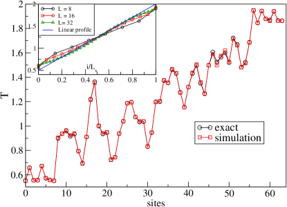
Figure 1: Temperature at all the sites of a $8\times 8$ fully disordered lattice, from simulations and from the exact solution. Inset shows the disorder-averaged temperature profiles for different system sizes and seems to approach a linear form.

Simulations with white noise: Equilibration times in simulations of disordered harmonic lattices can be very long and this can sometimes lead to wrong conclusions [see for e.g dharcom ]. To avoid such problems we first compare our simulation results with exact numerical results on steady state properties of small systems. We now briefly describe the numerical technique.

With $N=L_{x}L_{y}$ let us define the new variables $\{q_{1},q_{2},...,q_{2N}\}=\{x_{11},x_{12}...,x_{L_{x}L_{y}},p_{11},p_{12}...,p_{L_{x}L_{y}}\}$. Then Eq. 1 can be rewritten in the form:

$$\dot{q}_{l}=-\sum_{m=1}^{2N}{\bf a}_{lm}q_{m}+\xi_{l}$$ (3)

where the vector $\xi$ has all elements zero except $\xi_{N+j}=\eta^{L}_{j};~{}\xi_{2N-L_{y}+j}=\eta^{R}_{j}$ (for $1\leq j\leq L_{y}$) and the $2N\times 2N$ matrix ${\bf a}$ is given by:

$${\bf a}=\left(\begin{array}[]{cc}0&-{M}^{-1}\\ {\Phi}&{\Gamma}\end{array}\right)$$ (6)

where the $N\times N$ matrices ${M},{\Phi},~{}{\Gamma}$ can be labeled by the double indices $(i,j)$ and are given by

$${M}_{(ij),(i^{\prime}j^{\prime})}=\delta_{ii^{\prime}}\delta_{jj^{\prime}}m_{ij};~{}{\Phi}_{(ij)(i^{\prime}j^{\prime})}=4\delta_{ii^{\prime}}\delta_{jj^{\prime}}$$

$$~{}~{}~{}~{}~{}~{}-\delta_{ii^{\prime}}(\delta_{jj^{\prime}-1}+\delta_{jj^{\prime}+1})-\delta_{jj^{\prime}}(\delta_{ii^{\prime}-1}+\delta_{ii^{\prime}+1})$$

$${\Gamma}_{(ij)(i^{\prime}j^{\prime})}=\gamma\delta_{ii^{\prime}}\delta_{jj^{\prime}}(\delta_{i1}/m_{1j}+\delta_{iL_{x}}/m_{L_{x}j}).$$ (7)

In the steady state $\langle d(q_{n}q_{l})/dt\rangle=0$. From this and using Eq. 3 we get the matrix equation ried

$${\bf a}{\bf b}+{\bf b}{\bf a}^{T}={\bf d}=\left(\begin{array}[]{cc}0&0\\ 0&{\bf e}\end{array}\right)$$ (10)

where ${\bf b}$ is the correlation matrix with elements ${\bf b}_{nl}=\langle q_{n}q_{l}\rangle$ and ${\bf e}_{(ij)(i^{\prime}j^{\prime})}=\gamma\delta_{ii^{\prime}}\delta_{jj^{\prime}}(2T_{L}\delta_{i1}+2T_{R}\delta_{iL_{x}})$. Inverting this equation one obtains ${\bf b}$ and thus all the moments which includes the local temperatures $T_{ij}=\langle p_{ij}^{2}/m_{ij}\rangle$ and currents $J^{x}_{ij}=\langle x_{i-1j}p_{ij}/m_{ij}\rangle$. The dimension of the matrix which has to be inverted is $N(2N+1)\times N(2N+1)$ and using the fact that it is a sparse matrix we have been able to numerically superlu obtain ${\bf b}$ for system sizes up to $L_{x}=L_{y}=L=8$.

The molecular dynamics simulations were performed using a velocity-verlet scheme allen . We chose a step-size of $\Delta t=0.005$ and averaged over $10^{8}$ time steps (for $L=256$ we took $\Delta t=0.02$ and $10^{7}-5\times 10^{7}$ time steps). The temperatures at the two ends were set to $T_{L}=0.5$ and $T_{R}=2.0$. In Fig. 1, we plot $T_{ij}$ at every site, as obtained from the simulations and from the exact solution, for a particular realization of disorder. The agreement is clearly very good. We also find that that current fluctuations decay faster than fluctations of the local temperature. This is because, in the harmonic model, decay of fluctuations takes place only through coupling to the reservoirs and this is weak for localized modes that contribute to the temperature. This means that equilibrated values for the current can be obtained in smaller simulation runs.

Simulations were performed for sizes $L_{x}=L_{y}=L=4,8,16,...,256$ and in Fig. 2 we plot the system size-dependence of the current, averaged over $100$ samples ($9$ samples for $L=256$). Error-bars shown are those calculated from the disorder averaging, the thermal ones being much smaller. For larger system sizes we find that we need to average over a smaller number of realizations since the rms spread in the current decreases rapidly. From our data we estimate $\alpha=0.59\pm 0.01$.

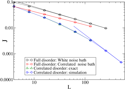
Figure 2: Plot of disorder-averaged-current versus system size for the two different heat baths and for the case of correlated disorder with white noise. For the full disorder cases, the solid lines are fits to the last three points and have slopes $0.59$ and $0.51$. For the case of correlated disorder, the slope from exact numerics (and also simulations) is compared to $1.5$ which is what one expects analytically.

We briefly note that Eq. 10 can be solved exactly for the ordered case, using methods similar to those in ried . The current is independent of system size and given by

$$J = \frac{(T_{L}-T_{R})}{4\pi\gamma}\int_{0}^{2\pi}dq\phi_{1}(q)$$

where $\phi_{1}(q)=1+\frac{1}{2}(\gamma^{-2}+\lambda_{q})-\frac{1}{2}[4(\gamma^{-2}+\lambda_{q})+(\gamma^{-2}+\lambda_{q})^{2}]^{1/2}$ and $\lambda=2[1-\cos(q)]$. The temperature in the bulk of the system takes the constant value $T=(T_{L}+T_{R})/2$.

Simulations with correlated noise: In this case the simulations were done by using a slightly modified version of the velocity-verlet algorithm with a step-size $\Delta t=0.001$ and averaging over $10^{8}$ time steps. The accuracy of the algorithm was tested in one-dimensions where exact numerical results are available dhar2 . Simulations were performed for sizes $L=4,8,16,...,128$ with disorder averages over $100$ samples ($22$ for $L=128$). The results are plotted in Fig. 2 and we estimate the exponent $\alpha=0.51\pm 0.01$ in this case, which is somewhat different from the slope of $\alpha\approx 0.59$ for the case of uncorrelated noise. It is possible that the small difference is a finite size effect and for larger system sizes we might see the same exponent. The error bars given are statistical errors while those from finite-size effects are more difficult to estimate. The next example throws some light on this aspect.

Correlated disorder: Finally we consider a special case of correlated disorder (with white noise baths) which was discussed in connor . This case is analytically tractable and gives us some insights on possible finite size effects. In this model, in a given column, say the $i$th, all particles have the same mass $m_{i}$. This case can be reduced to an effective one-dimensional problem connor . Using the fact that there is order in the transverse direction, we transform to new variables using an orthogonal basis $\psi_{j}(q)$ which satisfies the equation $2\psi_{j}(q)-\psi_{j-1}(q)-\psi_{j+1}(q)=\lambda_{q}\psi_{j}(q)$. We choose the $\psi_{j}(q)$ to be real and find that $\lambda_{q}=2(1-cos(q))$ with $q=2s\pi/L_{y}$ where $s=1,2,...,L_{y}$. The new variables $x_{i}(q)=\sum_{j}x_{i,j}\psi_{j}(q)$ satisfy the following equations of motion:

$$m_{1}\ddot{x}_{1}(q) = -\mu(q)x_{1}+x_{2}-\gamma\dot{x}_{1}+\eta^{L}(q)$$

$$m_{L_{x}}\ddot{x}_{L_{x}}(q) = -\mu(q)x_{L_{x}}+x_{L_{x}-1}-\gamma\dot{x}_{L_{x}}+\eta^{R}(q)$$

$$m_{i}\ddot{x}_{i}(q) = -\mu(q)x_{i}+x_{i-1}+x_{i+1}$$ (11)

(for $1<i<L_{x}$), where $\mu(q)=2+\lambda_{q}$. The transformed noise variables $\eta^{L}(q,t)=\sum_{j}\eta^{L}_{j}(t)\psi_{j}(q)$ satisfy $\langle\eta^{L}(q,t)\eta^{L}(q^{\prime},t^{\prime})\rangle=2T_{L}\gamma\delta(t-t^{\prime})\delta_{qq^{\prime}}$ and similarly for $\eta^{R}(q,t)$. Thus for every $q$ we have an equation identical to that of a one-dimensional disordered chain with an additional on-site potential $V=\lambda_{q}x^{2}/2$. The heat current in terms of the transformed variables is:

$$J=\frac{1}{L_{y}}\sum_{q}\langle(-\gamma\dot{x}_{1}(q)+\eta^{L}(q))\dot{x}_{1}(q)\rangle$$ (12)

Fourier transforming Eq. 11 using: $\tilde{x}_{i}(q,\omega)=\int dtx_{i}(q,t)e^{-i\omega t},~{}\tilde{\eta}^{L,R}(q,\omega)=\int dt\eta^{L,R}(q,t)e^{-i\omega t}$ we get the set of equations:

$$[\mu(q)-m_{1}\omega^{2}+i\gamma\omega]\tilde{x}_{1}-\tilde{x}_{2} = \tilde{\eta}^{L}$$

$$-\tilde{x}_{i-1}+[\mu(q)-m_{i}\omega^{2}]\tilde{x}_{i}-\tilde{x}_{i+1} = 0$$

$$-\tilde{x}_{L_{x}-1}+[\mu(q)-m_{L_{x}}\omega^{2}+i\gamma\omega]\tilde{x}_{L_{x}} = \tilde{\eta}^{R}$$

which in matrix notation can be written as ${\cal{Y}}(q,\omega)\tilde{x}(q,\omega)=\tilde{\eta}(q,\omega)$ where $\tilde{x}$, $\tilde{\eta}$ are the vectors $(\tilde{x}_{1}(q,\omega),...,\tilde{x}_{L_{x}}(q,\omega))^{T}$ and $(\tilde{\eta}^{L}(q,\omega),0,0,...,\tilde{\eta}^{R}(q,\omega))^{T}$. The matrix ${\cal{Y}}=k{\Phi}-\omega^{2}{M}+i\omega{\Gamma}$ where ${M}_{nl}=\delta_{nl}m_{n};~{}{\Phi}_{nl}=\mu(q)\delta_{nl}-\delta_{nl-1}-\delta_{nl+1}$ and ${\Gamma}_{nl}=\gamma\delta_{nl}(\delta_{n1}/m_{1}+\delta_{nL_{x}}/m_{L_{x}})$. After some manipulations the current in Eq. 12 simplifies to give:

$$J=\frac{\gamma^{2}(T_{L}-T_{R})}{\pi L_{y}}\sum_{q}\int_{-\infty}^{\infty}d\omega\omega^{2}|{\cal{Y}}^{-1}_{1L_{x}}(\omega,q)|^{2}$$ (13)

The inverse element is given by dhar2 : $|{\cal{Y}}^{-1}_{1L_{x}}(\omega,q)|^{2}=|Det[{\cal{Y}}]|^{-2}$ where $Det[{\cal{Y}}]=D_{1,L_{x}}+i\gamma\omega(D_{2,L_{x}}+D_{1,L_{x}-1})-\gamma^{2}\omega^{2}D_{2,L_{x}-1}$ and $D_{i,i^{\prime}}$ is defined to be the determinant of the submatrix of $k\hat{{\Phi}}-\omega^{2}{M}$ beginning with the $i$th row and column and ending with the $i^{\prime}$th row and column. These matrix elements can be expressed in terms of products of random matrices dhar2 . Using these results one can very efficiently compute the integral in Eq. 13 and obtain $J$ accurately for quite large system sizes ($L=512$). In Fig. 2 we show the system size dependence of the current as obtained from the exact numerical method and also from simulations. They agree very well and give $\alpha\approx{1.5}$. This value can be understood analytically by noting that the leading contribution to the current in Eq. 13 comes from the $q\to 0$ term (finite $q$ modes decay exponentially with system size) and this is identical to a pure $1D$ chain for which $\alpha=3/2$.

The fact that the simulation results agree extremely well with the exact numerical results (for sizes up to $L=128$) proves the accuracy of our simulations. Further we see that for the correlated disorder case the asymptotic result for the exponent can already be seen at around $L=512$. This gives us confidence that for the case of the fully disordered lattice we might already be close to the asymptotic value. This is also supported by the fact that the change in slope of the $J$-vesus-$L$ curves in Fig. 2 over the system sizes studied is very small.

Conclusions: We have performed extensive simulations of heat conduction in a mass-disordered harmonic solid in $2D$ which give exponents $\alpha\approx 0.59$ for white noise heat baths and $\alpha\approx 0.51$ for correlated noise baths. A system with correlated disorder gives, somewhat surprisingly, a larger exponent $\alpha=3/2$. The combination of simulations and exact numerics gives us confidence on the accuracy of our results and also additional insight. Some interesting open problems are the exact determination of the exponent $\alpha$ in $2D$, for any heat bath model, and an analytical understanding of dependence of $\alpha$ on bath properties.

We acknowledge A. P. Young for a critical reading of the manuscript. LWL acknowledges O. Narayan and T. Mai for useful discussions. The work of one of us (LWL) is supported by the NSF under grant DMR 0337049. We are grateful to the Hierarchical Systems Research Foundation (HSRF) for the usage of their computing cluster.

References

- (1) F. Bonetto, J.L. Lebowitz, L. Rey-Bellet, in Mathematical Physics 2000, edited by A. Fokas et al. (Imperial College Press, London, 2000), p. 128.
- (2) S. Lepri, R. Livi, and A. Politi, Phys. Rep. 377, 1 (2003).
- (3) T. Hatano, Phys. Rev. E 59, R1 (1999); A. Dhar, Phys. Rev. Lett. 86, 3554(2001); P. Grassberger, W. Nadler and L. Yang, Phys. Rev. Lett. 89, 180601 (2002); G. Casati and T. Prosen, Phys. Rev. E 67, 015203 (R) (2003); J. M. Deutsch and O. Narayan Phys. Rev. E 68, 010201(R) (2003).
- (4) O. Narayan and S. Ramaswamy, Phys. Rev. Lett. 89, 200601 (2002).
- (5) S. Lepri, R. Livi, and A. Politi, Europhys. Lett. 43, 271 (1998).
- (6) A. Dhar, Phys. Rev. Lett. 86, 5882 (2001).
- (7) A. J. O’Connor and J. L. Lebowitz, J. Math. Phys. 15, 692 (1974).
- (8) R. Rubin and W. Greer, J. Math. Phys. 12, 1686 (1971).
- (9) A. Casher and J. L. Lebowitz, J. Math. Phys. 12, 1701 (1971).
- (10) A. Lippi and R. Livi, J. Stat Phys. 100, 1147 (2000).
- (11) P. Grassberger and L. Yang, arXiv:cond-mat/0204247, (2002).
- (12) L. Yang, Phys. Rev. Lett. 88, 094301 (2002).
- (13) D. Frenkel and B. Smit, Understanding Molecular Simulation (Academic Press, 2002); A. Dhar (Unpublished notes).
- (14) B. Hu et al, Phys. Rev. Lett. 90, 119401 (2003).
- (15) R. H. H. Poetzsch and H. Bottger, Phys. Rev. B 50, 15757 (1994).
- (16) S. John, H. Sompolinsky and M. J. Stephen, Phys. Rev. B 27, 5592 (1983).
- (17) A. Dhar, Phys. Rev. Lett. 87, 069401 (2001).
- (18) Z. Rieder, J. L. Lebowitz, and E. H. Lieb, J. Math. Phys. 8, 1073 (1967).
- (19) J. W. Demmel, J. R. Gilbert and X. S. Li, SuperLU Users’ Guide (1999). LBNL Technical Report-44289.
- (20) M. P. Allen and D. L. Tildesley, Computer Simulation of Liquids (Clarendon Press Oxford, 1987).