Quantum and classical surface acoustic wave induced magnetoresistance oscillations in a 2D electron gas

Abstract

We study theoretically the geometrical and temporal commensurability oscillations induced in the resistivity of 2D electrons in a perpendicular magnetic field by surface acoustic waves (SAWs). We show that there is a positive anisotropic dynamical classical contribution and an isotropic non-equilibrium quantum contribution to the resistivity. We describe how the commensurability oscillations modulate the resonances in the SAW-induced resistivity at multiples of the cyclotron frequency.  We study the effects of both short-range and long-range disorder on the resistivity corrections for both the classical and quantum non-equilibrium cases. We predict that the quantum correction will give rise to zero-resistance states with associated geometrical commensurability oscillations at large SAW amplitude for sufficiently large inelastic scattering times. These zero resistance states are qualitatively similar to those observed under microwave illumination, and their nature depends crucially on whether the disorder is short- or long-range. Finally, we discuss the implications of our results for current and future experiments on two dimensional electron gases.

I Introduction

Recent experiments on high mobility two-dimensional electron gases (2DEGs) have shown a variety of magnetoresistance effects under intense microwave (MW) illumination. Zudov1 ; Mani1 ; Zudov2 ; Mani2 ; Willett2 ; Studenikin ; Yang ; KuKuMPL ; Dorozhkin ; Du One new phenomenon that has attracted considerable attention is MW-induced magnetoresistance oscillations. These are spaced according to the ratio of the MW frequency to the cyclotron frequency, showing a temporal commensurability between the MW field and the cyclotron motion. At high MW power the oscillations develop into zero resistance states (ZRS).Mani1 ; Zudov2 The phenomenological theory of ZRS by Andreev, Aleiner, and Millis Andreev has explained the effect to be a macroscopic manifestation of negative local resistivity imposed on the 2DEG by energy pumping from the microwave field. Several microscopic models have been proposed Aleiner ; Durst ; Mirlin ; ZRStheory to justify the periodic appearance of negative resistivity as a function of ratio of the MW frequency to the cyclotron frequency. The consensus is that the effect is of a quantum nature and related to the non-equilibrium occupation of Landau levels in a 2DEG pumped by microwave radiation.

A separate phenomenon involving geometrical commensurability oscillations has been extensively studied in 2D semiconductor structures subjected to either surface acoustic wave (SAW) or static modulations. SAW ; Willett ; Weiss ; Beenakker ; Gerhardts Commensurability between the diameter of the cyclotron orbit, $2R_{c}$ and the wavelength $2\pi/q$ of a coherent sound wave is known to manifest itself in magneto-oscillations of the dynamical conductivity $\sigma_{\omega q}$ of metals – the geometrical resonance effect. This was used in studies of three dimensional metals to determine the shape of the Fermi surface. Pippard Geometric resonance effects have also been observed in 2DEGs in the attenuation and renormalization of SAW velocity due to interactions with electrons Willett ; Shilton and in the drag effect due to SAWs. Shilton There has also been some theoretical study of these SAW-induced effects. Falko ; Efros ; Simon ; MW ; Halperin

In all of these studies, the parameter regimes used have been in the low frequency ($\omega\to 0$) limit, such that the SAWs are essentially static. Experiments have recently begun to investigate the effect of SAWs on magnetoresistance in a 2DEG. SAW We have studied this effect theoretically, investigating both geometric and temporal resonances. Robinson For a spatially periodic SAW field, the commensurability effect can also be viewed as a resonant SAW interaction with collective excitations of 2D electrons at finite wavenumbers, Willett ; Halperin enabling one to excite modes otherwise forbidden by Kohn’s theorem. Kohn These experimental developments require new theory for the response of a 2DEG to electric fields with both spatial and temporal modulation; this work was started in Ref. Robinson, and is continued here.

In this paper we study the non-linear dynamical effect in which SAWs induce changes in the magneto-resistivity of a high quality electron gas in the regime of classically strong magnetic fields, $\omega_{c}\tau\gg 1$ and high temperatures $k_{B}T\gg\hbar\omega_{c}$ ($\omega_{c}=eB/m^{*}$ is the cyclotron frequency, where $B$ is the magnetic field, $m^{*}$ the electron effective mass, and $\tau$ is the transport relaxation time). We have recently shown the existence of SAW-induced magnetoresistance oscillations Robinson that reflect both temporal and geometrical resonances in the SAW attenuation. There are two competing contributions to the resistivity corrections: one a classical SAW induced guiding centre drift of cyclotron orbits, the other a quantum contribution arising from the modulation of the electron density of states. In Ref. Robinson, , we restricted the analysis to 2DEGs with short-range disorder (which leads to isotropic scattering), so as to understand the main qualitative features of the oscillations. We also restricted our analysis of the quantum corrections to $\omega\lesssim\omega_{c}$. In the present work we extend our previous analysis of the quantum contribution to higher frequencies, $\omega\gtrsim\omega_{c}$, and address the experimentally relevant situation of long-range disorder which arises in modulation-doped systems and leads to small-angle scattering of electrons.

The classical contribution to the resistivity correction originates from the SAW-induced guiding centre drift of the cyclotron orbits. For a SAW with frequency $\omega$, and wavenumber $q$, propagating in the $x$ direction with speed $s=\omega/q$ (we assume $s$ is small compared to the Fermi velocity $\mathrm{v}_{F}$), there is an anisotropic increase in the resistivity $\rho_{xx}$ (at high fields $\omega_{c}\tau\gg 1,$ this is equivalent to an increase of conductivity in the transverse direction $\sigma_{yy}$), which oscillates as a function of inverse magnetic field. We show that at $\omega\gtrsim\omega_{c}$ the resistivity change displays resonances at integer multiples of the cyclotron frequency $\omega\approx N\omega_{c}$. We find that the main difference between long- and short-range disorder is that long-range disorder leads to an effective transport time $\tau^{*}=2\tau/(qR_{c})^{2}$ when $qR_{c}\gg\omega/\omega_{c}$. For small-angle scattering we obtain analytic formulae for the resistance correction for the limits $\omega_{c}\tau^{*}\gg 1$ when $(qR_{c})^{2}\ll\tau/\tau_{s}$, and $\omega_{c}\tau^{*}\ll 1$ for both $(qR_{c})^{2}\ll\tau/\tau_{s}$ and $(qR_{c})^{2}\gg\tau/\tau_{s}$, where $\tau_{s}$ is the total scattering time.MirlinW

The quantum contribution arises from the modulation of the electron density of states (DOS), $\tilde{\gamma}(\epsilon)$, and consequently, from the energy dependence of the non-equilibrium population of excited electron states caused by Landau level quantization. We follow the idea proposed in Ref. Aleiner, to explain the formation of ZRS Mani1 ; Zudov2 ; Andreev under microwave irradiation with $\omega\gtrsim\omega_{c}$. We show that in the frequency range $\tau^{-1}\lesssim\omega\lesssim\omega_{c}$ the quantum contribution suppresses resistivity both in $\rho_{xx}$ and $\rho_{yy}$ and persists up to temperatures $k_{B}T\gg\hbar\omega_{c}$ and filling factors $\nu\gg 1$ where no Shubnikov-de Haas (SdH) oscillations would be seen in the linear-response conductivity. We propose a new class of ZRS, in which geometric commensurability oscillations overlay the ZRS that would be found in the microwave ($qR_{c}\to 0$) limit for a short-range potential. For a long-range potential there are ZRS linked to geometric commensurability oscillations, which are enhanced (by $O([qR_{c}]^{2})$) over those induced by isotropic scattering.

The paper is organised as follows. In Sec. II we give qualitative arguments to determine the form of the classical magnetoresistance oscillations in the presence of short- and long-range disorder potentials. In Sec. III we obtain these results rigorously using the classical kinetic equation, and discuss screening of the SAW field. In Sec. IV we give our analysis of the quantum kinetic equation at both low and high frequencies. Finally, in Sec. V we discuss our results, in particular their implications for experiments.

II Qualitative analysis of Classical Magnetoresistance

It was shown by Beenakker Beenakker that the magnetoresistance oscillations in a 2DEG in the presence of a spatially modulated electric field can be understood from a semi-classical point of view by considering the guiding centre (${\mathbf{E}}\times{\mathbf{B}}$) drift of cyclotron orbits which lead to enhanced diffusion. We apply a similar method below to calculate the guiding center drift in the presence of an electric field with both temporal and spatial oscillations, for both isotropic scattering (short-range disorder) and small-angle scattering (long-range disorder). Note that the following qualitative analysis gives quantitative results applicable only to the high-field regime, $\omega_{c}\tau\gg 1$.

The dynamical classical resistivity change $\delta^{c}\rho_{xx}$ can be tracked back to the SAW induced drift $Y(t)$ (along the $y$-axis) of the guiding center ($X,Y$) of an electron cyclotron orbit Beenakker and the resulting enhancement of the transverse ($y$-) component of the electron diffusion coefficient, $D_{yy}$,

$$\dfrac{\delta^{c}\rho_{xx}}{\rho_{0}}=\dfrac{\delta D_{yy}}{D_{0}},$$

where $\rho_{0}=2/\gamma e^{2}{\mathrm{v}}_{F}^{2}\tau$ is the Drude resistivity and $D_{0}=R_{c}^{2}/2\tau$ is the unperturbed diffusion coefficient (where the cyclotron radius $R_{c}={\mathrm{v}}_{F}/\omega_{c}$). The drift is caused by an electric field $\tilde{E}_{\omega q}\cos(qx-\omega t)\hat{\mathbf{x}}$, where $x(t)$ is the position of the particle. To lowest order in $\tilde{E}_{\omega q}$, the contribution of the SAW to the guiding centre drift velocity is

$$\dot{Y}(t) \simeq \frac{\tilde{E}_{\omega q}}{B}\cos\left[qx(t)-\omega t\right],$$ (1)

$$\dot{X}(t) = 0,$$ (2)

where $x(t)$ is the position of the particle neglecting the effects of the SAW, but including the effects of disorder scattering. The change in the electron diffusion coefficient due to the SAW is then

$$\delta D_{yy}=\int_{0}^{\infty}\left<\dot{Y}(t)\dot{Y}(0)\right>dt,$$ (3)

where we average over all particle trajectories $x(t)$ in the disorder potential.

II.1 Short-range disorder: isotropic scattering

For isotropic scattering, the particle performs free cyclotron orbits, $x(t)=R_{c}\sin(\omega_{c}t+\phi_{0})+X_{0}$, up until a scattering event, after which the subsequent motion in the SAW potential is uncorrelated with its preceding motion, provided $qR_{c}\gg 1$. In this case, averaging over the trajectories and scattering events, the change in the diffusion coefficient due to the SAW is

$$\delta D_{yy}=\int_{0}^{\infty}\,dt\,e^{-t/\tau}\int_{0}^{2\pi}\int_{0}^{2\pi}\dfrac{d\phi_{0}}{2\pi}\dfrac{d\psi}{2\pi}\,\dot{Y}(t)\dot{Y}(0),$$ (4)

where $\psi=qX_{0}$, and $\dot{Y}(t)$ is calculated from Eq. (1) using the free cyclotron motion. Using the Bessel function identity

$$e^{iz\sin\phi}=\sum_{N=-\infty}^{\infty}J_{N}(z)e^{iN\phi},$$ (5)

one can obtain the frequency and wave number dependence of the magnetoresistance effect:

$$\frac{\delta^{c}\rho_{xx}}{\rho_{0}}=\frac{\delta D_{yy}}{D_{0}}=\frac{1}{4}\left(ql\tilde{\mathcal{E}}\right)^{2}\sum_{N=-\infty}^{\infty}\frac{J_{N}^{2}(qR_{c})}{1+\left(\omega-N\omega_{c}\right)^{2}\tau^{2}},$$ (6)

where

$$\tilde{\mathcal{E}}=ea_{\mathrm{scr}}\tilde{E}_{\omega q}^{\mathrm{SAW}}/\epsilon_{F},$$ (7)

is the dimensionless SAW amplitude. The electric field $\tilde{E}_{\omega q}$ discussed in this section is a travelling wave, rather than the standing wave situation discussed in Secs. III, IV and V. It is related to the $E_{\omega q}$ discussed in Sec. III by $\tilde{E}_{\omega q}=2E_{\omega q}$, implying $\tilde{\mathcal{E}}=2\mathcal{E}$. If we include another travelling wave to generate a standing wave, then the result in Eq. (6) should be multiplied by a factor of 2, and this reproduces Eq. (36). In Eqs. (6) and (7), $\tilde{E}_{\omega q}^{\mathrm{SAW}}$ is the SAW longitudinal electric field, $a_{\mathrm{scr}}=\chi/2\pi e^{2}\gamma$ the 2D screening radius, $\epsilon_{F}$ the Fermi energy, $l=\mathrm{v}_{F}\tau$ the mean free path, $\chi$ the background dielectric constant, and $\gamma=m/\pi\hbar^{2}$ the electron density of states. Equation (6) includes the Thomas-Fermi screening of the SAW field by 2D electrons, $\tilde{E}_{\omega q}=qa_{\mathrm{scr}}\tilde{E}_{\mathbf{\omega}q}^{\mathrm{SAW}}$, which we discuss in detail in Sec. III.1.1. At large $qR_{c}$ we can expand the Bessel functions to get

$$\frac{\delta^{c}\rho_{xx}}{\rho_{0}}\simeq\frac{1}{\pi qR_{c}}\left(ql\tilde{\mathcal{E}}\right)^{2}\sum_{N=-\infty}^{\infty}\frac{\cos^{2}\left(qR_{c}+\frac{N\pi}{2}-\frac{\pi}{4}\right)}{1+\left(\omega-N\omega_{c}\right)^{2}\tau^{2}}.$$ (8)

From Eqs. (6) and (8) we can see that there are a sequence of resonances at integer multiples of the cyclotron frequency, $\omega\approx N\omega_{c}$. The widths of these resonances are controlled by $\omega\tau$, with large values of $\omega\tau$ leading to very narrow resonances. The oscillations for even harmonics are in phase with the Weiss oscillations of the static potential, whilst those of odd harmonics are $\pi$ out of phase. This can be understood by noting that the main contributions to the drift occur when the electrons are moving parallel to equipotential lines. For odd harmonics the phase of the potential at the half-orbit point is opposite to that for a static potential, and hence the cancellation and reinforcement effects that lead to minima and maxima in the resistance are interchanged between the static and dynamic cases. This is illustrated via a comparison of the two situations in Fig. 1. Alternatively, this can be seen from examination of Eq. (8), since the static case ($\omega=0$) is dominated by the $N=0$ term in the sum, whereas all $N$ contribute in the dynamic case.

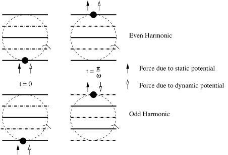
Figure 1: Comparison of electron motion in a static and a dynamic periodic potential. When the forces on opposite sides of the orbit are in the same direction, there is a maximum in the magnetoresistance. The horizontal lines correspond to maximum positive (solid lines) and maximum negative (dot-dashed lines) values of the field. In the dynamic case the direction of the field oscillates with frequency $\omega$. Thus, when $\omega$ is an odd multiple of the cyclotron frequency $\omega_{c}$, there is an interchange of the resistance maxima and minima as compared to a static potential.

In the regime $\omega_{c}\tau\gg{\mathrm{v}}_{F}/s$, the resonances are very narrow and appear to display a random sequence of heights, rather than the linear in $B$ dependence evident in Figs. 2 and 3, reflecting the dependence on the geometric resonance conditions. In the intermediate frequency domain, $\tau^{-1}\ll\omega\ll\omega_{c}$ , a natural regime for GaAs structures with densities $n_{e}\gtrsim 10^{10}\mathrm{cm}^{-2}$ at sufficiently high magnetic fields, the classical oscillations take the form

$$\frac{\delta^{c}\rho_{xx}}{\rho_{0}}\approx\frac{\mathrm{v}_{F}^{2}}{4s^{2}}\tilde{\mathcal{E}}^{2}J_{0}^{2}(qR_{c}).$$ (9)

The competition between electron screening effects ($\propto q^{2}$), the dynamical suppression of commensurability by the SAW motion ($\propto\omega^{-2}$), and the relation $\omega/q=s$, means that the form of these oscillations is independent of the absolute value of the SAW frequency, provided that conditions $\tau^{-1}\lesssim\omega$ and ${\mathrm{v}}_{F}\gg s$ are satisfied. Note however, that for a fixed SAW amplitude, there is still $q$ dependence of the SAW field $\tilde{E}^{\rm SAW}_{\omega q}$ since the electric field induced in the 2DEG by the piezoelectric coupling is a function of $qd$, where $d$ is the distance between the surface and the 2DEG. Simon2

Figure 2: Magnetoresistance for a short-range potential using the parameters of Ref. 1, and assuming $\omega=2\pi\times 10$ GHz ($\omega\tau=7$) and ${\mathrm{v}}_{F}/s=63$. We choose a dimensionless SAW amplitude of ${\mathcal{E}}=0.01$.

We illustrate the interplay between dynamical resonances in the time and space domains by plotting Eq. (6) as a function of $\omega_{c}/\omega$ for the following experimentally relevant parameters. In GaAs based 2DEGs, $m^{*}=0.068\,m_{e}$, (where $m_{e}$ is the electron mass) and $s\simeq 3000\,{\rm ms^{-1}}$. The highest SAW frequencies that have been used in experiments on 2DEGs are $\sim 10$ GHz; Willett3 we consider this fequency with the sample densities and mobilities reported in Refs. Zudov1, ; Zudov2, . In Ref. Zudov1, , the mobility $\mu$ is $3\times 10^{6}\,{\rm cm^{2}/Vs}$, and the density $n_{e}=2\times 10^{11}\,{\rm cm^{-2}}$, corresponding to $\omega\tau=7$ and ${\mathrm{v}}_{F}/s=63$ (note that ${\mathrm{v}}_{F}/s=qR_{c}$ when $\omega=\omega_{c}$). The magnetoresistance for these parameters is plotted in Fig. 2 In Ref. Zudov2, , $\mu=2.5\times 10^{7}\,{\rm cm^{2}/Vs}$ and $n_{e}=3.5\times 10^{11}\,{\rm cm^{-2}}$, making it one of the highest mobility samples yet fabricated. For these parameter values, $\omega\tau=60$, and ${\mathrm{v}}_{F}/s=84$, and we find a magnetoresistance trace as shown in Fig. 3. At lower frequencies in such a high quality 2DEG, we expect the width of the resonances to broaden and become similar to those shown in Fig. 2.

Figure 3: Magnetoresistance for a short-range potential using the parameters of Ref. 2, and assuming $\omega=2\pi\times 10$ GHz, which implies $\omega\tau=60$ and ${\mathrm{v}}_{F}/s=84$. We choose ${\mathcal{E}}=0.001$, a factor of 10 less than in Fig. 2.

The dynamical mechanism just described dominates in a classical electron gas. No redistribution of electron kinetic energy (due to SAW absorption) will additionally change the magnetoresistance until the 2DEG is heated to a temperature $k_{B}T_{e}\gtrsim\hbar\omega_{c}k_{F}/q$ where geometrical oscillations become smeared. The essential assumption leading to this statement is that electron single-particle parameters (velocity, ${\mathrm{v}}$, and $\tau^{-1}$) vary slowly with energy at the scales comparable to the Fermi energy and can thus be approximated by constants. However, for high-quality 2DEGs (as formed in modulation doped GaAs devices) the typical disorder potential is not simply short-range (as assumed for the isotropic scattering model considered above), but is dominated by a long-range part due to the coulombic potentials associated with remote dopants; this long-range disorder leads to small-angle scattering. We now turn to consider this situation.

II.2 Long-range random potential – small angle scattering

To calculate the resistivity correction in the presence of long range disorder, we consider an electron undergoing cyclotron motion and subject to random (small-angle) changes in direction. We express the position of the particle as

$${\mathbf{r}}(t)={\mathbf{R}}(t)+R_{c}(\sin\phi(t),\cos\phi(t)),$$ (10)

where ${\mathbf{R}}(t)$ is the position of the guiding centre and $\phi(t)$ is the angular position around the cyclotron orbit. In the absence of disorder, $\phi(t)=\phi_{0}+\omega_{c}t$ and ${\mathbf{R}}(t)$ is constant in time. The effect of a disorder potential on $\phi(t)$ may be represented by random changes: the scattering events are separated by a characteristic time $\tau_{s}$ (sometimes referred to as the quantum lifetime), and at each scattering event $\phi$ jumps through a (random) angle of magnitude $\delta\phi$, which is related to the lengthscale of the disorder potential $L$ by $\delta\phi\sim 1/(k_{F}L)$ where $k_{F}$ is the Fermi momentum. At any scattering event only the direction of motion changes; the position ${\mathbf{r}}(t)$ is constant, so Eq. (10) implies that for an instantaneous change $\delta\phi$ in $\phi$, there is a change in guiding centre position of

$$\delta{\mathbf{R}}=R_{c}(-\cos\phi,\sin\phi)\delta\phi.$$ (11)

In this section we consider the limit of a long range potential, for which $\delta\phi\ll 1$. In this case the scattering of $\phi$ can be viewed as leading to a continuous diffusive motion with a diffusion constant (in angle) of order $\sim(\delta\phi)^{2}/\tau_{s}$. Similarly, we can view the guiding centre co-ordinates as undergoing continuous diffusive motion, provided the typical jump [Eq. (11)] in guiding centre co-ordinate is small compared to other relevant lengthscales, in particular the wavelength of the SAW, $R_{c}\delta\phi\ll 1/q$. The diffusion constant for the guiding centre is $\sim R_{c}^{2}(\delta\phi)^{2}/\tau_{s}$. Note that the diffusion constants for $\phi$ and ${\mathbf{R}}$ depend only on the transport relaxation time $\tau\sim\tau_{s}/(\delta\phi)^{2}$, so only $\tau$ enters the theory. In terms of $\tau$, the conditions for validity of this theory ($\delta\phi\ll 1$, $R_{c}\delta\phi\ll 1/q$) can be written $\tau/\tau_{s}\gg 1$ and $(qR_{c})^{2}\ll\tau/\tau_{s}$.

To model the continuous diffusion of $\phi$ and ${\mathbf{R}}$, we introduce two sources of Gaussian noise, ${\mathcal{L}}_{1}$ and ${\mathcal{L}}_{2}$, with

$$\left<{\mathcal{L}}_{i}(t^{\prime}){\mathcal{L}}_{i}(t)\right>=\Gamma_{i}\delta(t-t^{\prime}),$$ (12)

(where $i=1,2$) and write the effects of scattering on the phase of the orbit and on the $x$-component of the guiding center position as

$$\phi(t) = \phi_{0}+\omega_{c}t+\int^{t}_{0}{\mathcal{L}}_{1}(t^{\prime})\,dt^{\prime},$$ (13)

$$X(t) = X_{0}+R_{c}\int_{0}^{t}{\mathcal{L}}_{2}(t^{\prime})\,dt^{\prime}.$$ (14)

The two sources of noise are related through Eq. (11)

$$\mathcal{L}_{2}(t)=-R_{c}\mathcal{L}_{1}(t)\cos\phi(t),$$

which requires that $\Gamma_{1}=2\Gamma_{2}$ in the situation of interest where we average over all trajectories (hence over $\phi_{0}$). From a direct evaluation of the classical Kubo formula for the diffusion constant for this model in the absence of a SAW potential, we find that

$$\Gamma_{1}=2\Gamma_{2}=\frac{2}{\tau},$$ (15)

where $\tau$ is the conventional definition of the transport relaxation time, in terms of which the Drude expression for diffusion constant is $D_{xx}=D_{yy}=\frac{1}{2}v_{F}^{2}\tau/(1+\omega_{c}^{2}\tau^{2})$.

We simplify subsequent calculations by ignoring correlations of ${\mathcal{L}}_{1}$ and ${\mathcal{L}}_{2}$ beyond those in Eq. (15), which we expect to be accurate for $\omega_{c}\tau^{*}\gg 1$, (with $\tau^{*}$ defined in Eq. (20) below) in which case the particle is able to explore all values of $\phi(t)$ on the timescale of the relevant scattering time. We can then calculate the change in the diffusion coefficient from the guiding centre drift as in Sec. II.1 for isotropic scattering, averaging over the electron trajectories

$$\delta D_{yy} = \int_{0}^{\infty}dt\left<\left<\dot{Y}(t)\dot{Y}(0)\right>\right>_{{\mathcal{L}}_{1},{\mathcal{L}}_{2}}$$ (16)

$$\simeq \frac{\tilde{E}_{\omega q}^{2}}{B^{2}}{\rm Re}\left\{\int_{0}^{\infty}dt\int_{0}^{2\pi}\frac{d\phi_{0}}{2\pi}\left<\left<e^{iqR_{c}(\sin\phi(t)-\sin\phi_{0})}\right.\right.\right.$$

$$\left.\left.\left.\hskip 28.45274pt\times\,e^{iqR_{c}\int^{t}{\mathcal{L}}_{2}(t^{\prime})dt^{\prime}-i\omega t}\right>\right>_{{\mathcal{L}}_{1},{\mathcal{L}}_{2}}\right\},$$

where our assumption that ${\mathcal{L}}_{1}$ and ${\mathcal{L}}_{2}$ are uncorrelated allows us to perform the average over noise:

$$\delta D_{yy} \propto \tilde{E}_{\omega q}^{2}{\rm Re}\left\{\int_{0}^{\infty}dt\,e^{-i\omega t}\int_{0}^{2\pi}\frac{d\phi_{0}}{2\pi}\right.$$

$$\left.\times\left<e^{iqR_{c}(\sin\phi(t)-\sin\phi_{0})}\right>_{{\mathcal{L}}_{1}}\left<e^{iqR_{c}\int^{t}{\mathcal{L}}_{2}(t^{\prime})dt^{\prime}}\right>_{{\mathcal{L}}_{2}}\right\}.$$

Using

$$\left<e^{iqR_{c}(\sin\phi(t)-\sin\phi_{0})}\right>_{{\mathcal{L}}_{1}} = \sum_{N,M=-\infty}^{\infty}J_{N}(qR_{c})J_{M}(qR_{c})$$

$$\hskip 11.38092pt\times\,e^{i(N-M)\phi_{0}}e^{iN\omega_{c}t}e^{-\frac{N^{2}\Gamma_{1}}{2}t},$$

$$\left<e^{iqR_{c}\int^{t}{\mathcal{L}}_{2}(t^{\prime})dt^{\prime}}\right>_{{\mathcal{L}}_{2}} = e^{-\frac{(qR_{c})^{2}}{2}\Gamma_{2}t},$$

we find a resistance correction of

$$\frac{\delta^{c}\rho_{xx}}{\rho_{0}}=\frac{{\mathrm{v}}_{F}^{2}\omega^{2}\tau}{4s^{2}}{\tilde{\mathcal{E}}}^{2}\sum_{N=-\infty}^{\infty}\frac{J_{N}(qR_{c})^{2}\,\tau_{Nq}}{1+(N\omega_{c}-\omega)^{2}\tau_{Nq}^{2}},$$ (18)

where

$$\tau_{Nq}=\frac{\tau}{N^{2}+\frac{(qR_{c})^{2}}{2}}.$$ (19)

The form of this correction is that found for isotropic scattering, but with $\tau_{Nq}$ replacing $\tau$ in the correction to the diffusion coefficient. footnote1 The result in Eq. (18) can be related to the result found in Eq. (58) in a similar manner to the case of short-range scattering.

In the experimentally relevant range of parameters, $\omega/\omega_{c}\ll qR_{c}$, and noting that in the vicinity of resonance $N$, $\omega/\omega_{c}\simeq N$, we define a scattering time $\tau^{*}\ll\tau$ as

$$\frac{1}{\tau^{*}}\equiv\frac{q^{2}R_{c}^{2}}{2\tau},$$ (20)

and $\tau_{Nq}\simeq\tau^{*}$ in our regime of interest. This quantity enters in our discussion of the kinetic equation for small-angle scattering in Sec. III.2. Note that the use of this result is also subject to the constraint $\omega_{c}\tau\gg 1$ with the additional requirement $qR_{c}^{2}\ll l$, which is discussed in more detail in Sec. III.

III Classical Kinetic Equation

We analyze the classical kinetic equation for a 2DEG at temperature $k_{B}T\lesssim\hbar\omega_{c}k_{F}/q$ irradiated by SAWs. Our approach is to solve the kinetic equation for the electron distribution function

$$f(t,x,\varphi,\epsilon)=f_{T}+\sum\limits_{\omega q}e^{-i\omega t+iqx}\sum_{m}f_{\omega q}^{m}(\epsilon)e^{im\varphi},$$ (21)

using the method of successive approximations. Here, $f_{T}(\epsilon)$ is the homogeneous equilibrium Fermi function, and the angle $\varphi$ and kinetic energy $\epsilon$ parametrize the electron state in momentum space. Each component $f^{m}$ describes the $m$-th angular harmonic of the time- and space-dependent non-equilibrium distribution. To describe local values of the electron current and the accumulated charge density, we use the energy-integrated functions, $g_{\omega q}^{m}=\int_{0}^{\infty}d\epsilon f_{\omega q}^{m}$. The relaxation of the local non-equilibrium distribution towards a Fermi function characterized by the value of local Fermi energy, $\epsilon_{F}(t,x)$ (determined by the local electron density $n(t,x)\propto g^{0}(t,x)=\int_{0}^{\infty}d\epsilon\,f^{0}(t,x)$, where $f^{0}(t,x)={\displaystyle\int}\dfrac{d\varphi}{2\pi}f(t,x)$) and the kinetic equation is

$$\mathcal{\hat{L}}f=\mathcal{\hat{C}}f,$$ (22)

where

$$\mathcal{\hat{L}}=\partial_{t}+\mathrm{v}\cos\varphi\,\partial_{x}+\left[\omega_{c}-\frac{eE}{p}\sin\varphi\right]\partial_{\varphi}+e\mathrm{v}E\cos\varphi\,\partial_{\epsilon},$$ (23)

with $\hat{\mathcal{C}}$ the collision integral, $E$ the electric field and $p$ the electron momentum.

III.1 Isotropic scattering

In the presence of a short-range potential, the scattering is isotropic and we can use the relaxation time approximation for the collision integral, which is

$$\mathcal{\hat{C}}f=-\dfrac{f-f^{0}}{\tau}-\dfrac{f^{0}-f_{T}(\epsilon-\epsilon_{F}(t,x))}{\tau_{in}},$$ (24)

where we distinguish between the elastic scattering rate $\tau^{-1}$ and energy relaxation rate $\tau_{in}^{-1}$.

The dynamical perturbation of the distribution function can be found from time/space Fourier harmonics of Eq. (22) at the frequency/wave number of the SAW,

$$\left[\partial_{\varphi}+\frac{1}{\omega_{c}\tau}-i\frac{\omega}{\omega_{c}}+iqR_{c}\cos\varphi\right]f_{\omega q}=\Psi(\varphi),$$ (25)

$$\Psi(\varphi) = -\frac{g_{\omega q}^{0}}{\omega_{c}\tau_{in}}(\partial_{\epsilon}f_{T})+\dfrac{\tau^{-1}-\tau_{in}^{-1}}{\omega_{c}}f_{\omega q}^{0}$$

$$-\frac{eE_{\omega q}}{\omega_{c}}[\mathrm{v}\cos\varphi\,\partial_{\epsilon}-\frac{\sin\varphi}{p}\partial_{\varphi}](f_{00}+f_{T}),$$

where we include the unknown perturbation of the time/space averaged function, $f_{00}$, related to the DC current to lowest order in $E_{\omega q}$. We note that as $\tau_{in}$ only contributes to heating of the 2DEG, we can ignore it here for the AC part of the distribution function, but must retain it for analysis of the DC part of the distribution function. In our expression for $\Psi$ we neglect contributions from higher Fourier harmonics of $f$, such as $f_{2\omega\,2q}$, $f_{2\omega\,0}$, and $f_{0\,2q}$, since these only affect DC transport at quartic order in the SAW field, whereas our interest is only in effects that are quadratic in the SAW field (i.e. linear in the SAW power). We also omit terms involving $E_{00}f_{\omega q}$, since they contribute to DC transport only beyond the linear response regime in the DC field. Equation (25) can be formally solved using the Green function $G(\varphi,\tilde{\varphi})$

$$f_{\omega q}(\varphi) = \int_{-\infty}^{\varphi}G(\varphi,\tilde{\varphi})\Psi(\tilde{\varphi})d\tilde{\varphi},$$ (26)

$$G(\varphi,\tilde{\varphi}) = e^{[\frac{1}{\omega_{c}\tau}-\frac{i\omega}{\omega_{c}}](\tilde{\varphi}-\varphi)+iqR_{c}[\sin\tilde{\varphi}-\sin\varphi]}\,,$$ (27)

which allows for an infinite range of variation of $\varphi$ whilst guaranteeing periodicity of the solution $f_{\omega q}(\varphi)$. We also introduce the useful quantity

$$K = \int_{0}^{2\pi}\dfrac{d\varphi}{2\pi}\int_{-\infty}^{\varphi}\dfrac{d\tilde{\varphi}}{\omega_{c}\tau}G(\varphi,\tilde{\varphi})$$ (28)

$$= \sum_{N=-\infty}^{\infty}\dfrac{J_{N}^{2}(qR_{c})}{1+i\tau(N\omega_{c}-\omega)}\quad,$$

which has the properties

$$K(\omega,q)=K^{\ast}(-\omega,q)=K(\omega,-q),$$

and is obtained from Eqs. (26) and (27) using Eq. (5).

III.1.1 Screening and Dispersive Resonance Shift

The electric field $E$ in Eq. (23) is the combination of a homogeneous DC field $\mathbf{E}_{00}$ and the screened electric field of the SAW, $\mathbf{E}(t,x)=\sum_{\omega q}E_{\omega q}e^{iqx-i\omega t}\hat{\mathbf{x}}$, found from the unscreened SAW field via $E_{\omega q}=E_{\omega q}^{\mathrm{SAW}}/\kappa(\omega,q)$, where $\kappa(\omega,q)$ is the dielectric function of the whole 2D structure. The density modulation $n_{\omega q}=\gamma g_{\omega q}^{0}$ induced by the SAW sets up an induced field $E_{\omega q}^{\mathrm{ind}}=-\frac{i2\pi eq}{\chi|q|}\gamma g_{\omega q}^{0},$ that we take into account at the level of Thomas-Fermi screening, so that $E_{\omega q}=E_{\omega q}^{\mathrm{SAW}}+E_{\omega q}^{\mathrm{ind}}$. In the analysis of screening, the DC part of the electric field can be ignored ($f_{00}=0$), and self-consistency yields

$$g_{\omega q}^{0} = \frac{eE_{\omega q}}{iq}\frac{1-(1-i\omega\tau)K}{1-K},$$ (29)

and

$$\kappa(\omega,q)=1+\frac{1}{a_{\mathrm{scr}}|q|}\frac{1-\left(1-i\omega\tau\right)K}{1-K}.$$ (30)

In the limit that $qR_{c}\gg 1$, which is our regime of interest, the dielectric function becomes

$$\kappa(\omega,q)=1+\frac{1-\left(1-i\omega\tau\right)K}{a_{\mathrm{scr}}|q|},$$ (31)

and for most SAWs, $a_{\mathrm{scr}}|q|\ll 1$, which implies $\kappa\simeq 1/(a_{\rm scr}|q|)$. When we account for dispersion, we find that the system has resonances at $\omega=N\omega_{c}+\Delta_{N}$ where $\Delta_{N}$ is the dispersive shift of the $N^{th}$ resonance.

We use Eq. (30) to find the eigenmodes of the system. Setting $\kappa=0$ and inserting the expression for $K$, one finds to leading order in $\omega_{c}\tau$,

$$\Delta_{N}=\dfrac{N\omega_{c}J_{N}^{2}(qR_{c})}{a_{\mathrm{scr}}|q|+1-J_{N}^{2}(qR_{c})-NA_{N}},$$ (32)

where

$$A_{N}=\sum_{p=1}^{\infty}\frac{J^{2}_{N-p}(qR_{c})-J^{2}_{N+p}(qR_{c})}{p}.$$ (33)

In the limit $qR_{c}\to 0$ we recover the magneto-plasmon dispersion, $\Delta_{1}\approx|q|R_{c}^{2}\omega_{c}/a_{\mathrm{scr}}$, whereas in the limit of $qR_{c}\gg 1$ screening becomes important and $\Delta_{N}\ll N\omega_{c}$. The crossover between the two regimes, which may be evaluated by considering the denominator of Eq. (32), occurs at a wavenumber $q_{0}R_{c}\sim a_{\mathrm{scr}}/R_{c}\ll 1$. In our discussion below we take into account the screening of the SAW field.

III.1.2 Magnetoresistance oscillations

To find the steady state current, we analyze the time/space average of the kinetic equation in Eq. (22) and take into account the dynamical perturbation $f_{\omega q}$

$${\displaystyle\left[\partial_{\varphi}+\frac{1}{\omega_{c}\tau}\right]f_{00}-\dfrac{\tau^{-1}-\tau_{in}^{-1}}{\omega_{c}}f_{00}^{0}+\frac{e\mathbf{v\cdot E}_{00}}{\omega_{c}}\partial_{\epsilon}f_{T}}$$

$$\hskip 17.07182pt{\displaystyle=-\sum_{\omega q}\frac{eE_{-\omega-q}}{\omega_{c}}\left[\mathrm{v}\cos\varphi\,\partial_{\epsilon}-\frac{\sin\varphi}{p}\partial_{\varphi}\right]f_{\omega q}.}$$ (34)

In our analysis of classical magnetoresistance oscillations we assume that $\tau_{in}\gg\tau$ and since we are not interested in the heating associated with this term we drop it here. However it is important for our analysis of the first quantum correction to the classical result that we present in Sec. IV. We substitute the solution Eq. (26) into Eq. (34), keeping track of the effect of the perturbation of the time/space averaged function $f_{00}$ on $f_{\omega q}$. This procedure automatically includes SAW-induced non-linear effects. We multiply Eq. (34) by $(2\omega_{c}/e\mathrm{v}_{F}^{2}){\mathrm{v}}e^{-i\varphi}$, integrate with respect to $\epsilon$ and $\varphi$, then use the relation between the $x$ and $y$ components of the DC current, $j_{x}-ij_{y}=e\gamma\mathrm{v}_{F}g_{00}^{1}$ and the harmonic $g_{00}^{1}$ (note that electrical neutrality requires $g_{00}^{0}=0$), which gives

$${\displaystyle\frac{2\omega_{c}}{e\mathrm{v}_{F}^{2}}\int\frac{d\varphi}{2\pi}e^{-i\varphi}\int d\epsilon\left\{\left[\partial_{\varphi}+\frac{1}{\omega_{c}\tau}\right]\mathrm{v}f_{00}\right.}$$ (35)

$${\displaystyle\hskip 14.22636pt\left.+\,\sum_{\omega q}\frac{\mathrm{v}eE_{-\omega-q}}{\omega_{c}}\left[\mathrm{v}\cos\varphi\,\partial_{\epsilon}-\frac{\sin\varphi}{p}\partial_{\varphi}\right]f_{\omega q}\right\}}$$

$$= {\displaystyle\frac{j_{x}}{\mathrm{v}_{F}^{2}\tau e^{2}\gamma/2}\frac{1}{2}\sum_{\omega q}\left|\frac{leE_{\omega q}}{\epsilon_{F}}\right|^{2}\frac{K}{1-K}}$$

$${\displaystyle\hskip 28.45274pt+\left(\frac{i\omega_{c}\tau+1}{\mathrm{v}_{F}^{2}\tau e^{2}\gamma/2}\right)[j_{x}-ij_{y}]}$$

$$= E_{00}^{x}-iE_{00}^{y},$$

and this can be used to determine the classical SAW induced change of the resistivity tensor, $\delta^{c}\hat{\rho}$. The relation between the electric field and current is $\mathbf{E}=\hat{\rho}\,\mathbf{j}+\delta^{c}\hat{\rho}\,\mathbf{j}$, where

$$\hat{\rho}=\rho_{0}\left(\begin{array}[]{cc}1&\omega_{c}\tau\\ -\omega_{c}\tau&1\end{array}\right),$$

is the Drude resistivity tensor. Thus we find the resistivity corrections

$$\frac{\delta^{c}\rho_{xx}}{\rho_{0}} = \frac{1}{2}\sum_{\omega q}\left|\frac{elE_{\omega q}}{\epsilon_{F}}\right|^{2}\mathrm{Re}\left\{\frac{K}{1-K}\right\},$$ (36)

$$\delta^{c}\rho_{yy} = 0,$$

$$\dfrac{\delta^{c}\rho_{yx}}{\rho_{0}} = \dfrac{\delta^{c}\rho_{xy}}{\rho_{0}}=-\frac{1}{2}\sum_{\omega q}\left|\frac{leE_{\omega q}}{\epsilon_{F}}\right|^{2}\mathrm{Im}\left\{\frac{K}{1-K}\right\}=0,$$

and with the use of $E_{\omega q}=E_{\omega q}^{\mathrm{SAW}}/\kappa(\omega,q)\simeq qa_{scr}E^{\rm SAW}_{\omega q}$, Eq. (28), $\omega_{c}\tau\gg 1$ and $qR_{c}\gg 1$ we formally justify the result in Eq. (6). The magnetoresistance correction is:

$$\frac{\delta^{c}\rho_{xx}}{\rho_{0}}=2\left(ql\mathcal{E}\right)^{2}\sum_{N=-\infty}^{\infty}\frac{J_{N}^{2}(qR_{c})}{1+\left(\omega-N\omega_{c}\right)^{2}\tau^{2}}.$$ (37)

Strong damping ($\omega_{c}\tau\ll 1$)

At low magnetic fields, there is experimental Beton and theoretical MirlinW ; Boggild evidence that there is exponential damping of Weiss oscillations, and it seems natural that similar behaviour should be observed for SAW-induced oscillations. We explore this question and find the functional form of the damping for isotropic scattering in this section, and for small angle scattering in Sec. III.2. In the strong damping limit ($\omega_{c}\tau\ll 1$), we investigate Eq. (28) when $qR_{c}\gg 1$ and find the values of $\varphi$ and $\tilde{\varphi}$ that lead to a stationary phase. We then integrate over fluctuations about each point of stationary phase. These saddle points are $\varphi=\pi/2$ and $\varphi=3\pi/2$, and $\tilde{\varphi}$ takes values which are any positive or negative odd integer multiplying $\pi/2$ such that $\tilde{\varphi}\leq\varphi$. When we sum the results of integrating about each saddle point, we get (to lowest order in $e^{-\frac{\pi}{\omega_{c}\tau}}$)

$$K=\frac{1}{\omega_{c}\tau}\left[\frac{1}{|qR_{c}|}+\frac{2}{qR_{c}}e^{-\frac{\pi}{\omega_{c}\tau}+\frac{i\pi\omega}{\omega_{c}}}\sin(2qR_{c})\right].$$ (38)

In the limit that the magnetic field goes to zero, with $ql\gg 1$, this leads to a resistance change

$$\left.\frac{\delta^{c}\rho_{xx}}{\rho_{0}}\right|_{B=0}=2ql{\mathcal{E}}^{2},$$ (39)

and if we consider the resistance change $\delta\rho_{xx}$, we find it is

$$\delta^{c}\rho_{xx}=\frac{h^{2}}{\pi e^{2}}\frac{q}{p_{F}}{\mathcal{E}}^{2},$$ (40)

which is independent of disorder. Summation over $\pm\omega$ and taking the imaginary part of $K$ as in Eq. (36) leads to the same result that $\delta^{c}\rho_{xy}=0$.

We interpret this as a SAW-induced backscattering contribution to the resistance, which will dominate in the limit that the SAW wavelength is much less than the mean free path. We ignore the contribution to the resistance from channeled orbits, which can also lead to a positive contribution to the magnetoresistance in the small magnetic field limit. Menne ; Beton2 The condition for the existence of these orbits is that the force from the screened SAW field is larger than the Lorentz force, i.e. ${\mathcal{E}}>\frac{\omega_{c}}{\omega}\frac{s}{\mathrm{v}_{F}}$,MirlinW ; Menne and we assume that ${\mathcal{E}}$ is sufficiently small for their contribution to be ignored (this is generally the case over most of the magnetic field range that we show in our figures).

III.2 Small angle scattering

A long range disorder potential leads to a non-isotropic scattering probability, and this implies that there are two scattering times that we need to take into account. One is the total scattering time, $\tau_{s}$,MirlinW and the other is the momentum scattering time, $\tau$, and in GaAs heterostructures, $\tau\gg\tau_{s}$. In the limit that $(qR_{c})^{2}\ll\frac{\tau}{\tau_{s}}$, the disorder potential leads to diffusion in angle, and can be studied by replacing the collision integral in the kinetic equation by a term involving two $\varphi$ derivatives. MirlinW The dynamical perturbation of the distribution function, Eq. (25) is thus modified to read

$$\left[\partial_{\varphi}-i\frac{\omega}{\omega_{c}}+iqR_{c}\cos\varphi-\frac{1}{(\omega_{c}\tau)^{2}}\partial_{\varphi}^{2}\right]f_{\omega q}=\tilde{\Psi}(\varphi),$$ (41)

where

$$\tilde{\Psi}(\varphi)=-\frac{eE}{\omega_{c}}\left[{\mathrm{v}}\cos\varphi\,\partial_{\epsilon}-\frac{\sin\varphi}{p}\partial_{\varphi}\right]\left(f_{00}+f_{T}\right).$$ (42)

In Eq. (41), small angle scattering is introduced in the form of diffusion along the Fermi surface and is taken into account by the term $\frac{1}{\tau}\partial_{\phi}^{2}f$. Now, if we let $f_{\omega q}=h_{\omega q}(\varphi)e^{-iqR_{c}\sin\varphi}$, and substitute this into Eq. (41), then solve in the limits that $qR_{c}/\omega_{c}\tau\ll 1$ and $\omega/\omega_{c}\ll qR_{c}$ (the second condition allows us to ignore the term $\partial_{\varphi}^{2}h$), we can solve the kinetic equation as before to get

$$f_{\omega q}(\varphi)=\int^{\varphi}_{-\infty}d\tilde{\varphi}\,\tilde{G}(\varphi,\tilde{\varphi})\tilde{\Psi}(\tilde{\varphi}),$$ (43)

where

$$\tilde{G}\left(\varphi,\tilde{\varphi}\right) = \exp\bigg{\{}iqR_{c}\left(\sin\tilde{\varphi}-\sin\varphi\right)$$ (44)

$$\hskip 14.22636pt\left.+\left(\frac{1}{\omega_{c}\tau^{*}}-i\frac{\omega}{\omega_{c}}\right)\left(\tilde{\varphi}-\varphi\right)\right.$$

$$\hskip 14.22636pt\left.-\frac{1}{2\omega_{c}\tau^{*}}\left(\sin 2\varphi-\sin 2\tilde{\varphi}\right)\right\},$$

and $\tau^{*}$ was defined in Eq. (20). Our results for isotropic scattering are modified by replacing $G$ by $\tilde{G}$. The long-range potential problem is then reduced to a calculation of $\tilde{K}$ for the modified Green function, which we define in analogy with Eq. (28) as

$$\tilde{K}=\int_{0}^{2\pi}\frac{d\varphi}{2\pi}\int^{\varphi}_{-\infty}\frac{d\tilde{\varphi}}{\omega_{c}\tau^{*}}\,\tilde{G}(\varphi,\tilde{\varphi}).$$ (45)

We can write the following exact expression for $\tilde{K}$:

$$\tilde{K} = \sum_{s,m,p=-\infty}^{\infty}\frac{J_{s+2m-2p}(qR_{c})J_{s}(qR_{c})}{1+i((s+2m)\omega_{c}-\omega)\tau^{*}}$$ (46)

$$\hskip 8.5359pt\times\,e^{\frac{i\pi}{2}(m+p)}I_{m}\left(\frac{1}{2\omega_{c}\tau^{*}}\right)I_{p}\left(\frac{1}{2\omega_{c}\tau^{*}}\right),$$

where $I_{m}(x)$ is the modified Bessel function of the first kind. We study $\tilde{K}$ in the weak damping ($\omega_{c}\tau^{*}\gg 1$) and the strong damping ($\omega_{c}\tau^{*}\ll 1$) limits.

Weak damping ($\omega_{c}\tau^{*}\gg 1$)

In the weak damping limit, we can make use of the asymptotic expansion of the modified Bessel functions for small argument, and need only retain the $m=p=0$ terms. $\tilde{K}$ has the same form as $K$, except that $\tau$ is replaced by $\tau^{*}$, i.e.

$$\tilde{K}=\sum_{N=-\infty}^{\infty}\dfrac{J_{N}^{2}(qR_{c})}{1+i(N\omega_{c}-\omega)\tau^{*}}\quad,$$ (47)

where $\frac{1}{\tau^{*}}=\frac{(qR_{c})^{2}}{2\tau}$ was introduced in Eq. (20).

Strong damping ($\omega_{c}\tau^{*}\ll 1$)

In the strong damping limit when $qR_{c}\gg 1$ and $(qR_{c})^{2}\ll\frac{\tau}{\tau_{s}}$, we investigate Eq. (45) and use a similar saddle point procedure to the one we used for strong damping in the case of isotropic scattering. After adding the contributions from integrating about each saddle point, we get (to lowest order in $e^{-\frac{\pi}{\omega_{c}\tau^{*}}}$)

$$\tilde{K}=\frac{1}{\omega_{c}\tau^{*}}\left[\frac{1}{|qR_{c}|}+\frac{2}{qR_{c}}e^{-\frac{\pi}{\omega_{c}\tau^{*}}+\frac{i\pi\omega}{\omega_{c}}}\sin(2qR_{c})\right].$$ (48)

Note that this is the same form as the expression for $K$ for isotropic scattering in the limit $\omega_{c}\tau\ll 1$, except that $\tau$ replaces $\tau^{*}$. If we want to investigate the limit in which the magnetic field goes to zero, then the kinetic equation [Eq. (41)] as written previously is inapplicable when $(qR_{c})^{2}\gg\frac{\tau}{\tau_{s}}$.MirlinW In our calculation above, there is a damping factor of $D=e^{-\frac{\pi}{\omega_{c}\tau^{*}}}$, which arises naturally as a result of our saddle point analysis. In Ref. MirlinW, an alternative approach was used to calculate the damping factor in the low magnetic field limit. In that approach the damping factor above is the high field limit of

$$D_{1}=\exp\left\{-\frac{\pi}{\omega_{c}\tau_{s}}\left[1-\frac{1}{\sqrt{1+\frac{\tau_{s}}{\tau}(qR_{c})^{2}}}\right]\right\},$$ (49)

where $\tau_{s}$ is the total relaxation rate. If, as in Sec. II.2, we assume that phase and guiding center corrections are uncorrelated, we can calculate a second damping factor associated with phase corrections in addition to the guiding center contribution in Eq. (49), using the same method. This gives

$$D_{2}=\exp\left\{-\frac{\pi}{\omega_{c}\tau_{s}}\frac{\left(\frac{\omega}{\omega_{c}}\right)^{2}}{1+\left(\frac{\omega}{\omega_{c}}\right)^{2}\frac{\tau_{s}}{\tau}}\right\},$$ (50)

and at moderate fields, we may approximate $D=D_{1}D_{2}$, so that

$$\tilde{K}=\frac{1}{\omega_{c}\tau^{*}}\left[\frac{1}{|qR_{c}|}+\frac{2}{qR_{c}}De^{\frac{i\pi\omega}{\omega_{c}}}\sin(2qR_{c})\right].$$ (51)

If we assume that the two effects are correlated (as we should in the $(qR_{c})^{2}\gg\frac{\tau}{\tau_{s}}$ limit), then we get the expression

$$D=\exp\left\{-\frac{1}{\omega_{c}\tau_{s}}\int_{0}^{\pi}d\phi\frac{(ql\sin\phi-\omega\tau)^{2}}{(ql\sin\phi-\omega\tau)^{2}+(\omega_{c}\tau)(\omega_{c}\tau_{s})}\right\},$$ (52)

which implies that in the $\omega_{c}\tau\to 0$ limit, with $ql\gg\omega\tau\gg 1$ and $\frac{\tau}{\tau_{s}}\gg 1$

$$D\simeq\exp\left\{-\frac{\pi}{\omega_{c}\tau_{s}}\left[1-\frac{\omega\tau}{(ql)^{2}}\omega_{c}\tau\sqrt{\frac{\tau_{s}}{\tau}}\right]\right\},$$ (53)

which gives $\lim_{\omega_{c}\to 0}D=e^{-\frac{\pi}{\omega_{c}\tau_{s}}}\neq\lim_{\omega_{c}\to 0}D_{1}D_{2}=e^{-\frac{2\pi}{\omega_{c}\tau_{s}}}$.

III.2.1 Screening

In the above discussion, the solutions obtained for $f_{\omega q}$ in Sec. III.1 and for $f_{\omega q}$ when there is small-angle scattering differ in that the kinetic equation for isotropic scattering contained the term $g^{0}_{\omega q}/\omega_{c}\tau$, which is absent here. When we solve for $g^{0}_{\omega q}$, and hence the dielectric function, Eq. (30), in the presence of small-angle scattering, we get

$$g_{\omega q}^{0} = \frac{eE_{\omega q}}{iq}\left[1-(1-i\omega\tau^{*})\tilde{K}\right],$$ (54)

which implies a dielectric function

$$\kappa(\omega,q)=1+\frac{1-\left(1-i\omega\tau^{*}\right)\tilde{K}}{a_{\mathrm{scr}}|q|},$$ (55)

which is very similar to Eq. (31) with $\tilde{K}$ replacing $K$. When $qR_{c}\gg 1$, screening of SAWs is identical for both short and long range potentials. Analysis of $\Delta_{N}$ and $A_{N}$ as in Sec. III.1.1 leads to the same $q_{0}$ at which screening becomes important.

III.2.2 Magnetoresistance oscillations

In this section we derive the magnetoresistance oscillations analogously to Sec. III.1.2. The system of equations that we wish to solve is

$${\displaystyle\partial_{\varphi}f_{0}+\frac{eE_{\omega q}}{\omega_{c}}\left[{\mathrm{v}}\cos\varphi\,\partial_{\epsilon}-\frac{\sin\varphi}{p}\partial_{\varphi}\right]f_{\omega q}}$$

$${\displaystyle\hskip 14.22636pt=-\frac{e{\mathbf{v}}\cdot{\mathbf{E}}_{0}}{\omega_{c}}\partial_{\epsilon}f_{T}+\frac{1}{\omega_{c}\tau}\partial^{2}_{\varphi}f_{0}},$$ (56)

in combination with Eqs. (41) and (42). The solution of Eq. (41) for $f_{\omega q}$, is shown in Eq. (43). We take the equation for $f_{0}$, and integrate with respect to energy and $\varphi$ after multiplying by ${\mathrm{v}}e^{-i\varphi}$, as before, and obtain

$$\delta E^{x}_{00}-i\delta E^{y}_{00} = \frac{2\omega_{c}}{em^{2}{\mathrm{v}}_{F}^{3}}\left(\frac{eE_{\omega q}}{\omega_{c}}\right)^{2}(g^{1}_{0}+g^{-1}_{0})$$

$$\hskip 8.5359pt\times\int_{0}^{2\pi}\frac{d\varphi}{2\pi}\int^{\varphi}_{-\infty}d\tilde{\varphi}\,\tilde{G}(\varphi,\tilde{\varphi}),$$

which is the same as we found for isotropic scattering, except that $\tilde{G}$ replaces $G$. The resistivity correction is thus

$$\frac{\delta^{c}\rho_{xx}}{\rho_{0}}=\frac{1}{2}\sum_{\omega q}\left|\frac{elE_{\omega q}}{\epsilon_{F}}\right|^{2}\frac{\tau^{*}}{\tau}{\rm Re}\left\{\tilde{K}\right\}.$$ (57)

As in the case of short-range scattering there are no corrections to any other components of the resistivity tensor. Unlike the case of isotropic scattering there is not a factor of $1-\tilde{K}$ in the denominator of Eq. (57) – this is because the resistivity correction is linear in $g^{0}_{\omega q}$, which is modified for small-angle scattering [see Eq. (54)].

Thus our results for the classical contribution to the magnetoresistance can be summarized as follows. For weak damping, $\omega_{c}\tau^{*}\gg 1$, and $1\ll(qR_{c})^{2}\ll\frac{\tau}{\tau_{s}}$ the resistivity correction is:

$$\frac{\delta^{c}\rho_{xx}}{\rho_{0}}=\frac{2{\mathrm{v}}_{F}^{2}\omega^{2}\tau\tau^{*}}{s^{2}}{\mathcal{E}}^{2}\sum_{N=-\infty}^{\infty}\frac{J_{N}^{2}(qR_{c})}{1+\left(\omega-N\omega_{c}\right)^{2}{\tau^{*}}^{2}}\,.$$ (58)

For strong damping, $\omega_{c}\tau^{*}\ll 1$, and $1\ll(qR_{c})^{2}\ll\frac{\tau}{\tau_{s}}$,

$$\frac{\delta^{c}\rho_{xx}}{\rho_{0}}=2ql{\mathcal{E}}^{2}\left[1+2e^{-\frac{\pi}{\omega_{c}\tau^{*}}}\cos\left(\frac{\pi\omega}{\omega_{c}}\right)\sin(2qR_{c})\right],$$

(59)

whilst for $\omega_{c}\tau^{*}\ll 1$ and $(qR_{c})^{2}\gg\frac{\tau}{\tau_{s}}$,

$$\frac{\delta^{c}\rho_{xx}}{\rho_{0}}=2ql{\mathcal{E}}^{2}\left[1+2e^{-\frac{\pi}{\omega_{c}\tau_{s}}}\cos\left(\frac{\pi\omega}{\omega_{c}}\right)\sin(2qR_{c})\right].$$

(60)

Summation over $\pm\omega$ and $\pm q$ for the imaginary part of $\tilde{K}$ ensure that $\delta^{c}\rho_{xy}$ and $\delta^{c}\rho_{yy}$ vanish as for short range scattering [see Eq. (36)]. The three resistivity regimes identified above correspond respectively to high [Eq. (58)], intermediate [Eq. (59)], and low [Eq. (60)] magnetic fields. The crossover between high and intermediate magnetic fields is at $\omega_{c}\tau^{*}\sim 1$, which is equivalent to $\omega_{c}\tau\sim(ql)^{\frac{2}{3}}$, and the crossover between intermediate and low magnetic fields is when $(qR_{c})^{2}\sim\frac{\tau}{\tau_{s}}$, which is equivalent to $\omega_{c}\tau\sim ql\sqrt{\frac{\tau_{s}}{\tau}}$. The number of damped oscillations at low magnetic field has recently been calculated elsewhere.Robinson2 As for short range scattering, these results are for the regime where channeled orbits can be ignored, which requires that the Lorentz force should be stronger than the screened SAW field, i.e. ${\mathcal{E}}<\frac{\omega_{c}}{\omega}\frac{s}{\mathrm{v}_{F}}.$

Both Eqs. (58) and (59) reduce to the results found by Mirlin and Wölfle MirlinW in the limit that $\omega\to 0$, provided one replaces $\omega/s$ by $q$ in Eq. (58). To extrapolate this result to lower magnetic fields, the best we can do is a similar procedure to Mirlin and Wölfle, which is to replace $e^{-\frac{\pi}{\omega_{c}\tau^{*}}}$ by the damping factor $D$ discussed in Sec. III.2, leading to Eq. (60). In the limit that $B\to 0$ this reduces to the same behaviour as in the case of isotropic scattering, and the magnetoresistance correction is given by Eq. (40). We neglect the possibility of channeled orbits, as discussed in Sec. III.1.2.

Figure 4: Magnetoresistance correction for small-angle scattering, with $\omega\tau=7$, ${\mathrm{v}}_{F}/s=63$, and ${\mathcal{E}}=0.02$. The curve is determined by splicing the expressions for the resistance in the strong and weak damping limits ($\omega_{c}\tau^{*}<1$ and $\omega_{c}\tau^{*}>1$ respectively), which are indicated in the figure.

In Figs. 4, 5, and 6 we show the behaviour of the magnetoresistance as determined by splicing the results of Eq. (58) and Eq. (59) for the weak and strong damping cases respectively. In Fig 4 we use the same sample parameters as in Fig. 2, whilst both Figs. 5 and 6 are for ${\mathrm{v}}_{F}/s=84$, with $\omega\tau=60$ in Fig. 5 and $\omega\tau=600$ in Fig. 6; for the sample parameters in Ref. Zudov2, these correspond to $\omega=2\pi\times 10$ GHz and $2\pi\times 100$ GHz respectively. Note that, owing to our requirement $qR_{c}\ll\omega_{c}\tau$, our results should not be trusted in the region $\omega_{c}/\omega\lesssim\sqrt{{\mathrm{v}}_{F}/(s\omega\tau)}$ (which is of order 1 for the parameters used), i.e. at low magnetic fields. However, our expectation is that magnetoresistance oscillations should be strongly damped in this regime, as described in Eq. (60). We also note that for $\omega_{c}/\omega\gg 1$, the resistance correction in the case of small-angle scattering is enhanced over that expected for isotropic scattering with the same value of the transport time (i.e. the same 2DEG mobility).

Figure 5: Magnetoresistance correction for small-angle scattering, with $\omega\tau=60$, ${\mathrm{v}}_{F}/s=84$, and ${\mathcal{E}}=0.003$. The curve is determined by splicing the expressions for the resistance in the weak and strong damping limits, which are indicated in the figure.

Figure 6: Magnetoresistance correction for small-angle scattering, with $\omega\tau=600$, ${\mathrm{v}}_{F}/s=84$, and ${\mathcal{E}}=0.002$. The curve is a splice of the formulae for the strong and weak damping limits, and the range of validity for each region is indicated.

IV Quantum Kinetic contribution to SAW-induced magnetoresistance

The absorption of SAWs by electrons in two dimensions changes their steady state distribution over energy. Characteristics that are independent of energy cause no additional changes to magnetoresistance beyond those previously described. However, when $\omega_{c}\tau\gg 1$, Landau level quantization is present, leading to an oscillatory energy-dependence of the electron DOS for overlapping Landau levels of $\tilde{\gamma}(\epsilon)=\left[1-\Gamma\cos\left(2\pi\epsilon/\hbar\omega_{c}\right)\right]\gamma$, where $\Gamma=2e^{-\frac{\pi}{\omega_{c}\tau_{q}}}\ll 1$, and $\tau_{q}$ is the quantum lifetime of the Landau levels. Ando [A calculation of the density of states for a long-range disorder potentialRaikh shows that $\tau_{q}$ can be field-dependent.] This gives rise to a quantum contribution to the geometrical commensurability oscillations which can persist up to high temperatures. The oscillations in the DOS impose oscillations on the electron elastic scattering rate, $\tau^{-1}(\epsilon)=\tau^{-1}\tilde{\gamma}(\epsilon)/\gamma$, which in turn gives a contribution to the observable conductivity. At low temperatures, $k_{B}T\lesssim\hbar\omega_{c}$, the DOS oscillations lead to Shubnikov-de Haas (SdH) oscillations in conductivity. At high temperatures $k_{B}T\gg\hbar\omega_{c}$, thermal broadening smears out the SdH oscillations, but the quantum contribution can remain as a non-linear effect after energy averaging.

We follow a similar approach to Dmitriev et al. Mirlin ; Aleiner to study the quantum kinetic equation to obtain the first quantum correction to the classical magnetoresistance induced by SAWs. This change in the distribution is oscillatory in energy and leads to a contribution to the DC conductivity that oscillates as a function of $\omega/\omega_{c}$. The effect depends on the efficiency of energy relaxation and hence is proportional to $\tau_{in}$; this effect dominates the quantum corrections discussed in Refs. Durst, when $\tau_{in}/\tau_{q}\gg 1$. If this is the case, the energy relaxation time is long compared to the Landau level lifetime, allowing a strongly non-equilibrium electron distribution as a function of energy to arise.

The photoconductivity $\sigma_{\rm ph}$ determines the longitudinal current flowing in response to a DC electric field in the presence of SAWs:

$${\mathbf{j}}\cdot{\mathbf{E}}_{00}=\sigma_{\rm ph}|{\mathbf{E}}_{00}|^{2},$$ (61)

and can be related to the photoresistivity by $\rho_{\rm ph}\simeq\rho_{xy}^{2}\sigma_{\rm ph}$, where $\rho_{xy}=eB/n_{e}$. To calculate the photoconductivity, one integrates over the distribution function

$$\sigma_{\rm ph}=2\int d\epsilon\,\sigma_{00}(\epsilon)\left[-\partial_{\epsilon}f(\epsilon)\right],$$ (62)

and in the leading approximation,

$$\sigma_{00}(\epsilon)=\sigma_{00}^{D}\frac{\tilde{\gamma}^{2}(\epsilon)}{\gamma^{2}},$$ (63)

where

$$\sigma^{D}_{00}=\frac{e^{2}\gamma{\mathrm{v}}_{F}^{2}}{2\omega_{c}^{2}\tau},$$ (64)

is the Drude conductivity. In obtaining a solution to the problem, we are only interested in effects due to the non-trivial energy dependence of the electron distribution function $f(\epsilon)$.

To perform this calculation we need the classical dynamical conductivity, from which we consider the energy dependence of the density of states $\gamma$ and the momentum relaxation time $\tau$. We calculate the classical dynamical conductivity below in Sec. IV.1, and then use it to derive the quantum energy balance equation and magnetoresistance correction in Sec. IV.2.

IV.1 Classical dynamical conductivity

The magnetic field dependence of the resistivity change reflects the form of the SAW attenuation by the 2D electrons determined by the real part of the longitudinal dynamical conductivity $\sigma_{\omega q}$,

$$\mathrm{Re}\left\{\sigma_{\omega q}\right\}=\gamma s^{2}\tau e^{2}\,\mathrm{Re}\left\{\frac{K}{1-K}\right\}\mathrm{.}$$ (65)

We obtain $\sigma_{\omega q}$ from considering attenuation in the form

$$\left\langle\mathbf{E}_{\omega q}\cdot\mathbf{j}_{\omega q}\right\rangle=\sigma_{\omega q}|E_{\omega q}|^{2},$$

and we use the expression in Eq. (65) in the following subsection. In analogy with our previous work, we find that the equation for $\sigma_{\omega q}$ for small-angle scattering is

$$\mathrm{Re}\left\{\sigma_{\omega q}\right\}=\gamma s^{2}\tau^{*}e^{2}\,\mathrm{Re}\left\{\tilde{K}\right\}.$$ (66)

IV.2 Quantum energy balance equation

The quantum energy balance equation in Ref. Aleiner, is stated without detailed derivation. Here we provide a simple derivation as an alternative to the approach used in Ref. Aleiner, . If we consider the energy balance in a 2DEG due to absorption and emission of SAWs, then the rate at which energy is added is $Q(t)={\mathbf{j}}_{\omega q}(t)\cdot{\mathbf{E}}_{\omega q}(t),$ and ${\mathbf{j}}_{\omega q}(t)=\sigma_{\omega q}{\mathbf{E}}_{\omega q}(t)$, which when we average over time gives $\bar{Q}=\frac{1}{2}\sigma_{\omega q}|{\mathbf{E}}_{\omega q}|^{2}$ We can express the rate of absorption or emission processes involving energy levels $i$ and $j$ as

$$\Gamma_{ij}=\frac{2\pi}{\hbar}|M_{ij}|^{2}\delta(\epsilon_{i}-\epsilon_{j}\pm\hbar\omega),$$ (67)

using Fermi’s golden rule, where $M_{ij}$ is the matrix element between states $i$ and $j$. We assume that $M_{ij}=M$ and calculate the total power absorption for the classical case ($\gamma$ constant), which we equate to $\bar{Q}=\frac{1}{2}\sigma_{\omega q}|{\mathbf{E}}_{\omega q}|^{2}.$ Hence

$$\bar{Q}=\frac{2\pi}{\hbar}|M|^{2}\hbar\omega\gamma(\hbar\omega\gamma),$$ (68)

where one factor of $\hbar\omega$ is the energy added per photon absorbed, $\gamma$ is the final density of states, and $\hbar\omega\gamma$ is the number of electrons below the Fermi level that are available to make a transition. This gives a formula for $|M|^{2}$:

$$|M|^{2}=\frac{\hbar\bar{Q}}{2\pi(\hbar\omega\gamma)^{2}}.$$ (69)

We now consider the change in the number of electrons with energy $\epsilon\to\epsilon+d\epsilon$ allowing the density of states to be energy dependent, $\tilde{\gamma}(\epsilon)$:

$$\begin{array}[]{l}{\displaystyle\frac{d}{dt}\left[f(\epsilon)\tilde{\gamma}(\epsilon)d\epsilon\right]}\\ {\displaystyle=\frac{2\pi}{\hbar}|M|^{2}\left\{\sum_{\pm}f(\epsilon\pm\hbar\omega)\tilde{\gamma}(\epsilon\pm\hbar\omega)d\epsilon\,\tilde{\gamma}(\epsilon)(1-f(\epsilon))\right.}\\ \hskip 56.9055pt{\displaystyle-f(\epsilon)\tilde{\gamma}(\epsilon)d\epsilon\,\tilde{\gamma}(\epsilon\pm\hbar\omega)(1-f(\epsilon\pm\hbar\omega))\Bigg{\}}}\\ \hskip 8.5359pt{\displaystyle-\frac{f(\epsilon)-f_{T}(\epsilon)}{\tau_{in}}\tilde{\gamma}(\epsilon)d\epsilon.}\end{array}$$ (74)

(75)

When we require that the distribution be stationary, the left hand side of the equation vanishes and when we divide by $\tilde{\gamma}(\epsilon)$ we get

$$\frac{\sigma_{\omega q}|E_{\omega q}|^{2}}{2\hbar^{2}\omega^{2}\gamma^{2}}\sum_{\pm}\tilde{\gamma}(\epsilon\pm\hbar\omega)\left[f(\epsilon\pm\hbar\omega)-f(\epsilon)\right]=\frac{\left[f(\epsilon)-f_{T}(\epsilon)\right]}{\tau_{in}}.$$ (76)

If we want to include the effects of a DC field as well, then we can see the form of the DC term from the $\omega\to 0$ limit of the right hand side of Eq. (75), and we get as a final result the balance equation from Ref. Aleiner, ,

$$\frac{\sigma_{\omega q}|E_{\omega q}|^{2}}{2\hbar^{2}\omega^{2}\gamma^{2}}\sum_{\pm}\tilde{\gamma}(\epsilon\pm\hbar\omega)\left[f(\epsilon\pm\hbar\omega)-f(\epsilon)\right]$$

$$+\frac{|E_{00}|^{2}\sigma_{00}}{\tilde{\gamma}(\epsilon)}\frac{\partial}{\partial\epsilon}\left[\frac{\tilde{\gamma}(\epsilon)^{2}}{\gamma^{2}}\frac{\partial}{\partial\epsilon}f(\epsilon)\right]=\frac{\left[f(\epsilon)-f_{T}(\epsilon)\right]}{\tau_{in}}.$$ (77)

We could also have obtained the same equation by treating $\sigma_{\omega q}$ as energy dependent and then pulling out factors of the energy dependent density of states from $\tilde{\gamma}(\epsilon)$ and $\tau^{-1}(\epsilon+\hbar\omega)$, which is equivalent to the approach in Ref. Mirlin, . This second approach works provided $|N-\omega/\omega_{c}|\leq 1/\omega_{c}\tau$ (i.e. we can ignore the 1 in the denominator of the sum over $N$ harmonics in $\sigma_{\omega q}$). At frequencies closer to resonance than this, we can no longer ignore the 1 in the denominator and the classical expression lacks accuracy. However, for large $\omega_{c}\tau$ this is a relatively small region of magnetic fields, and is not relevant at the magnetic fields at which ZRS mimima are observed.

We use the expression for $\sigma_{\omega q}$ from Eq. (65) (short-range disorder potential) or Eq. (66) (long-range disorder potential), which contains the geometric and frequency commensurability oscillations, and $\sigma_{00}^{D}$ we know as the Drude resistivity [Eq. (64)]. Introduce the following quantities

$${\mathcal{P}} = \tau_{in}\frac{2\sigma_{\omega q}|E_{\omega q}|^{2}}{\hbar^{2}\omega^{2}\gamma},$$ (78)

$${\mathcal{Q}} = \tau_{in}\frac{4\pi^{2}\sigma^{D}_{00}|E_{00}|^{2}}{\hbar^{2}\omega_{c}^{2}\gamma}.$$ (79)

We are then left with the following equation to solve

$${\displaystyle\frac{{\mathcal{P}}}{4}\sum_{\pm}\left(1-\Gamma\cos\left(\frac{2\pi(\epsilon\pm\hbar\omega)}{\hbar\omega_{c}}\right)\right)\left(f(\epsilon\pm\hbar\omega)-f(\epsilon)\right)}$$

$${\displaystyle+\frac{\hbar^{2}\omega_{c}^{2}\gamma}{4\pi^{2}\tilde{\gamma}(\epsilon)}{\mathcal{Q}}\frac{\partial}{\partial\epsilon}\left[\left(1-\Gamma\cos\left(\frac{2\pi\epsilon}{\hbar\omega_{c}}\right)\right)^{2}\frac{\partial}{\partial\epsilon}f(\epsilon)\right]}$$

$$=f(\epsilon)-f_{T}(\epsilon).$$

Now, let $f(\epsilon)=f_{0}(\epsilon)+\Gamma f_{1}(\epsilon)\cos\left[\frac{2\pi\epsilon}{\hbar\omega_{c}}\right]$, where $f_{0}(\epsilon)\simeq f_{T}(\epsilon)$, so $f(\epsilon)\simeq f_{T}(\epsilon)+f_{\rm osc}(\epsilon)$. When we do this, and then sum over $\omega$ and neglect all derivatives of $f_{1}$ that arise from Taylor expanding $f(\epsilon\pm\hbar\omega)$ (since this is assumed to be a smooth function on the energy scale of $k_{B}T$), and retain only lowest order terms in $\Gamma$, we get a linear equation in $f_{\rm osc}$ which is trivial to solve and leads to (noting that $\partial_{\epsilon}^{2}f_{T}$ is also ignored) an identical result to Ref. Aleiner, :

$$f_{\rm osc}=\frac{\hbar\omega_{c}}{2\pi}\frac{\Gamma}{2}\frac{\partial f_{T}}{\partial\epsilon}\sin\left(\frac{2\pi\epsilon}{\hbar\omega_{c}}\right)\frac{\frac{2\pi\omega}{\omega_{c}}{\mathcal{P}}\sin\left(\frac{2\pi\omega}{\omega_{c}}\right)+4{\mathcal{Q}}}{1+{\mathcal{P}}\sin^{2}\left(\frac{\pi\omega}{\omega_{c}}\right)+{\mathcal{Q}}}.$$ (81)

We then use the expression for the photoconductivity, Eq. (62) and get the isotropic change in the DC conductivity

$$\frac{\sigma_{\rm ph}}{\sigma_{00}^{D}}=1+\frac{\Gamma^{2}}{2}\left[1-\frac{\frac{2\pi\omega}{\omega_{c}}{\mathcal{P}}\sin\left(\frac{2\pi\omega}{\omega_{c}}\right)+4{\mathcal{Q}}}{1+{\mathcal{P}}\sin^{2}\left(\frac{\pi\omega}{\omega_{c}}\right)+{\mathcal{Q}}}\right].$$ (82)

Note that in the approach outlined above we made no detailed assumptions about the momentum relaxation apart from $\tau_{in}\gg\tau$, such that the momentum relaxation is efficient in making the distribution isotropic. Thus the only difference in the expression for a short or long-ranged potential is in the form of $\sigma_{\omega q}$, which enters in the expression for ${\mathcal{P}}$ in Eq. (78). We now present numerical calculations of the resistivity change derived above in the presence of SAWs for both isotropic and small-angle scattering. All these calculations are for the case ${\mathcal{Q}}=0$.

IV.3 Numerical results

In this section we show the resistivity as it is modified by the quantum correction alone. We discuss the situation where both classical and quantum corrections are important in Sec. V.1.

IV.3.1 Isotropic scattering

We illustrate numerical results for the magnetoresistance oscillations due to the combination of SAWs and density of states modulations in Fig. 7. We use Eq. (28) for $K$ and do not ignore the 1 in the denominator of the summand. For large $\omega\tau$, this should give accurate results except for a very small range of magnetic fields around each of the resonances where $\omega/\omega_{c}$ equals an integer. Note that we divide the expression in Eq. (82) by $1+\Gamma^{2}/2$, to compare the resistivity with and without SAWs, assuming that there are density of states modulations in both cases. To connect to our previous notation, we note that

$${\mathcal{P}}=2\left(\frac{\epsilon_{F}}{\hbar\omega}\right)^{2}(\omega\tau)(\omega\tau_{in}){\mathcal{E}}^{2}{\rm Re}\left\{\frac{K}{1-K}\right\}.$$ (83)

In Fig. 7 we show the change in the magnetoresistance for $\omega\tau_{q}=6$ and $\omega\tau_{in}=302$ (using the value of $\tau_{in}=7.64\times 10^{-10}$ s estimated in Ref. Aleiner, ) for the parameters that we calculated the classical magnetoresistance corrections displayed in Figs. 2 and 3. As for the case of a microwave field, there are peaks in the resistance when $\omega/\omega_{c}$ is close to an integer, but with $\delta\rho_{xx}=0$ when $\omega/\omega_{c}$ is exactly equal to an integer. The peaks (and dips) are modulated by geometric commensurability oscillations, and this leads to a new class of ZRS, of the type predicted for $\omega\ll\omega_{c}$ in Ref. Robinson, . For $\omega\tau=7$, ${\mathrm{v}}_{F}/s=63$, the ZRS occur for ${\mathcal{E}}\gtrsim 0.0015$ and for $\omega\tau=60$, ${\mathrm{v}}_{F}/s=84$, ZRS occur for ${\mathcal{E}}\gtrsim 0.001$.

Figure 7: Quantum contribution to the magnetoresistance for $\omega\tau=7$, ${\mathrm{v}}_{F}/s=63$ and $\omega\tau=60$, ${\mathrm{v}}_{F}/s=84$, both with $\omega\tau_{q}=6$, ${\mathcal{E}}=0.0015$, and $\omega\tau_{in}=302$.

At large $\omega_{c}/\omega\gg 1$ (not shown) the resistance change is negative as we predicted analytically previously.Robinson However, the magnitude of the resistance change is very much smaller than when $\omega/\omega_{c}\gtrsim 1$, so a very large value of ${\mathcal{E}}$ would be required to attain ZRS at $\omega_{c}/\omega\gg 1$.

IV.3.2 Small angle scattering

In Fig. 8 we show data for the quantum magnetoresistance correction when there is small-angle scattering for the same sample parameters and frequencies as in Figs. 4 and 5. Similarly to the short-range case, we can relate ${\mathcal{P}}$ to our previous notation:

$${\mathcal{P}}=2\left(\frac{\epsilon_{F}}{\hbar\omega}\right)^{2}(\omega\tau^{*})(\omega\tau_{in}){\mathcal{E}}^{2}{\rm Re}\left\{\tilde{K}\right\},$$ (84)

where the change from Eq. (83) reflects that we use a different $\sigma_{\omega q}$ in the two cases.

Figure 8: Quantum contribution to magnetoresistance for $\omega\tau=7$, ${\mathrm{v}}_{F}/s=63$ and for $\omega\tau=60$, ${\mathrm{v}}_{F}/s=84$. In both cases $\omega\tau_{q}=6$, ${\mathcal{E}}=0.003$, and $\omega\tau_{in}=302$. The arrows indicate the range of validity of the results.

If $\omega_{c}/\omega\lesssim 1$ then there are ZRS of the type that are usually observed with microwaves, however there are another class of magnetoresistance oscillations at larger values of $\omega_{c}/\omega$, which are of the sort we predicted in Ref. Robinson, , and are much less strongly damped than in the isotropic scattering case. We note that for $\omega\tau=60$, ${\mathrm{v}}_{F}/s=84$, the threshold value for ZRS at $\omega_{c}/\omega>1$ is ${\mathcal{E}}\simeq 0.003$. In Fig. 8 we clearly demarcate the values of $\omega_{c}/\omega$ where our analytic formulae are valid ($qR_{c}/\omega_{c}\tau\ll 1$).

V Discussion

V.1 Combination of classical and quantum effects

At low frequencies ($\omega\ll\omega_{c}$) we can use the approach in Sec. IV.2 to obtain an analytic expression for the quantum resistivity correction, starting with the low frequency limit of the balance equation for vanishing dc field. This calculation was already considered in Ref. Robinson, , and we quote the result here for completeness. We find a non-vanishing addition to both diagonal components of the conductivity (and, therefore, also of the resistivity) even when $k_{B}T\gg\hbar\omega_{c}$. This generates isotropic magneto-oscillations for short-range disorder

$$\dfrac{\delta^{q}\rho_{\alpha\alpha}}{\rho_{0}}=\dfrac{\delta^{q}\sigma_{\alpha\alpha}}{\sigma_{0}}=-\frac{2\tau_{in}}{\tau}\left|\frac{4\pi\Gamma\epsilon_{F}}{\hbar\omega_{c}}\right|^{2}\mathcal{E}^{2}J_{0}^{2}\left(qR_{c}\right),$$ (85)

(where $\sigma_{0}=1/\rho_{0}$) in addition to the anisotropic classical commensurability effect. Together, they yield the result:

$$\frac{\delta\rho_{xx}}{\rho_{0}} \approx \frac{\delta\sigma_{yy}}{\sigma_{0}}=2J_{0}^{2}\left(qR_{c}\right)\mathcal{E}^{2}\left[\frac{\mathrm{v}_{F}^{2}}{s^{2}}-\frac{\tau_{in}}{\tau}\left(2\pi\Gamma\nu\right)^{2}\right],$$

$$\frac{\delta\rho_{yy}}{\rho_{0}} \approx \frac{\delta\sigma_{xx}}{\sigma_{0}}=-2J_{0}^{2}\left(qR_{c}\right)\mathcal{E}^{2}\frac{\tau_{in}}{\tau}\left(2\pi\Gamma\nu\right)^{2},$$ (86)

valid when $\tau^{-1}\lesssim\omega\ll\omega_{c}$, where $\nu=2\epsilon_{F}/\hbar\omega_{c}$ is the filling factor. For a long-range potential, the oscillations are very similar, for ${\tau^{*}}^{-1}\lesssim\omega\ll\omega_{c}$, with $\tau^{*}$ replacing $\tau$ to give

$$\frac{\delta\rho_{xx}}{\rho_{0}} \approx \frac{\delta\sigma_{yy}}{\sigma_{0}}=2J_{0}^{2}\left(qR_{c}\right)\mathcal{E}^{2}\left[\frac{\mathrm{v}_{F}^{2}}{s^{2}}\frac{\tau}{\tau^{*}}-\frac{\tau_{in}}{\tau^{*}}\left(2\pi\Gamma\nu\right)^{2}\right],$$

$$\frac{\delta\rho_{yy}}{\rho_{0}} \approx \frac{\delta\sigma_{xx}}{\sigma_{0}}=-2J_{0}^{2}\left(qR_{c}\right)\mathcal{E}^{2}\frac{\tau_{in}}{\tau^{*}}\left(2\pi\Gamma\nu\right)^{2}.$$ (87)

The actual magnetoresistance trace observed in an experiment will have both anisotropic classical and isotropic quantum contributions. The parameter that controls the overall behaviour for both isotropic scattering and small-angle scattering is

$$\eta\equiv\left(2\pi\Gamma\nu s/\mathrm{v}_{F}\right)\sqrt{\tau_{in}/\tau}.$$ (88)

We can use $\eta$ to identify three different magnetoresistance regimes. If $\eta<1$, the observed change in the resistivity is in the direction of SAW propagation. If $\eta\simeq 1$, then the observed change in the resistivity is in the direction perpendicular to the SAW wavevector, and if $\eta\gg 1$, then the resistance correction is isotropic and negative. For the parameter values used in Figs. 7 and 8, the parameter $\eta$ is large compared to one, such that the quantum contribution dominates the classical corrections.

The quantum contribution to the resistivity that we discuss in Sec. IV is not the only possible contribution to the resistivity that can arise from quantum effects neglected in a classical calculation. A static periodic potential affects the equilibrium density of states, which can lead to corrections to $\rho_{yy}$ as well as to $\rho_{xx}$.Gerhardts ; Gerhardts2 These corrections were ignored in our calculations, but at least in the static case appear to be at most the order of magnitude of the classical contribution. Hence the quantum effect we discuss here should dominate that quantum correction for $\eta>1$, provided $\tau_{in}\gg\tau$ and $\nu>{\mathrm{v}}_{F}/2\pi s$.

V.2 Experimental Implications

There are four situations we have discussed in this paper: the combinations of either short- or long-range disorder and quantum and classical corrections to the magnetoresistance due to SAWs. We first focus on the case of isotropic scattering. The most pronounced geometric and temporal oscillations in the magnetoresistance are in the region $\omega_{c}/\omega\lesssim 1$ regardless of whether the oscillations are quantum or classical in origin. The classical effects dominate for short inelastic scattering times and lead to anisotropic, positive magnetoresistance corrections, whilst quantum effects dominate for large inelastic scattering times, and can lead to ZRS which are modulated by geometric commensurability oscillations. For small-angle scattering, geometric commensurability oscillations in the regime $\omega_{c}/\omega\lesssim 1$ are very strongly damped in both the classical and quantum cases, unless $(qR_{c})^{2}/\omega_{c}\tau\lesssim 1$ in this region. This condition is not met in current high quality 2DEGs in which small-angle scattering dominates. However, it is currently possible to achieve $(qR_{c})^{2}/\omega_{c}\tau\lesssim 1$ for $\omega_{c}/\omega>1$, and these geometric commensurability oscillations should be observable either in the quantum or classical regimes when $\omega_{c}/\omega>1$. Similarly to isotropic scattering, quantum effects dominate for large inelastic scattering times (compared to the elastic scattering time) and classical effects are more important for short inelastic scattering times. It appears that the ZRS at low frequencies we predicted in Ref. Robinson, for isotropic scattering, are hard to achieve if the scattering is isotropic, but should be much more readily achievable in samples where small-angle scattering dominates, which is the experimentally relevant situation.

One theoretical prediction for ZRS is that they require inhomogeneous current flow in a 2DEG, Andreev which appears to have recently been observed for microwaves.Willett2 A large enough SAW-induced change $\left|\delta\sigma_{xx}\right|>\sigma_{0}$ resulting in negative local conductivity would also require the formation of electric field/Hall current domains. Since the anisotropy in Eq. (86) suggests that such conditions can be achieved most easily in the conductivity component along the SAW wavevector, we expect that domains would form with current flowing perpendicular to the direction of SAW propagation, and their stability would depend on the sample geometry. For a SAW with the wavevector directed across the axis of a Hall bar, current domains can be stabilized by ending in ohmic contacts. For a wave propagating (or standing) along the Hall bar, current domains would have to orient across the bar direction and terminate at the sample edges (destabilizing them), leading to a finite resistance. Finally, the anisotropy would not support a zero-conductance regime in a Corbino geometry.

In addition to the parameter ranges that are optimal for observing SAW-induced ZRS, there are several other experimental issues we would like to mention. Firstly there is the observation by Kukushkin et al. KuKuMPL that microwave irradiation of high quality 2DEGs can lead to SAW generation. Thus one might want to consider the effects of microwaves and SAW simultaneously – such a scheme might also allow for probing a 2DEG at frequencies other than $qs$ for a given SAW wavenumber. However, this calculation is beyond the scope of the present work.footnote2

If increases in SAW frequency and 2DEG mobility allow $\omega\tau\gg(qR_{c})^{2}$ for $\omega/\omega_{c}\geq 1$, the geometric oscillatory structure similar to that observed for isotropic scattering i.e. peaks when $\omega/\omega_{c}$ is an integer should be visible in both classical and quantum contributions to magnetoresistance. This is currently not yet observable for samples in which small-angle scattering dominates (as appears to be the case for the samples used in Refs. Mani1, ; Zudov2, where ZRS were observed) because $\omega_{c}\tau^{*}\gg 1$ when $\omega/\omega_{c}\gtrsim 1$. Either samples in which isotropic scattering dominates are required to see these effects, or higher quality samples in which $(qR_{c})^{2}/\omega_{c}\tau\gg 1$ when $\omega/\omega_{c}>1$ are required. In terms of trying to improve the possibility of observing interesting SAW induced magnetoresistance effects in the frequency range $\omega\gtrsim\omega_{c}$ in samples where small-angle scattering dominates, the following considerations may be helpful. Since ${\mathrm{v}}_{F}/s\propto n_{e}^{\frac{1}{2}}$ and $\omega\tau\propto\omega\mu$ (and it is found that $\mu\propto n_{e}^{0.7}$ in the highest quality GaAs/AlGaAs 2DEGs Pfeiffer ), the best hope for observing effects with $\omega\tau\gg{\mathrm{v}}_{F}/s$ appears to be by achieving higher SAW frequencies.

V.3 Conclusions

In conclusion, we have demonstrated a new class of magnetoresistance oscillations caused in a 2DEG by SAWs. We have shown that at $\omega\ll\omega_{c}$ the effect consists of contributions with competing signs: (i) a classical geometric commensurability effect analogous to that found in static systems with positive sign, and (ii) a quantum correction, with negative sign for either isotropic or small-angle scattering. The latter result suggests that SAW propagation through a high mobility electron gas may generate a sequence of zero-resistance states (ZRS) linked to the maxima of $J_{0}^{2}\left(qR_{c}\right)$ for strong enough SAW fields. We find that in the region $\omega\ll\omega_{c}$, SAW-induced ZRS states are much more likely to be observed in samples for which small-angle scattering dominates isotropic scattering. Whilst this prediction concerns the low-frequency domain $\omega\lesssim\omega_{c}$, such ZRS would be formed via the same mechanism Andreev ; Aleiner as the microwave-induced ZRS at $\omega\gtrsim\omega_{c}$. In the regime $\omega\gtrsim\omega_{c}$, we find that there are geometric oscillations superposed on ZRS if there is isotropic scattering. If there is small-angle scattering, such oscillations are unlikely to be seen in 2DEGs at the present time. Hence the optimal parameter region to search for SAW induced ZRS in 2DEGs with long-range disorder which show geometric modulation is for $\omega<\omega_{c}$ and $(qR_{c})^{2}/\omega_{c}\tau<1$.

We thank I. Aleiner, D. Khmelnitskii, and A. Mirlin for discussions. This work was funded by EPSRC grants GR/R99027, GR/R17140, and the Lancaster Portfolio Partnership. It progressed during the Workshop “Quantum transport and correlations in mesoscopic systems and Quantum Hall Effect” at the Max-Planck-Institut PKS in Dresden, the Workshop on “Quantum Systems out of Equilibrium” at the Abdus Salam ICTP in Trieste, and V. F.’s research visit to ICTP.

References

- (1) M. A. Zudov, R. R. Du, J. A. Simmons, and J. R. Reno, Phys. Rev. B 64, 201311(R) (2001).
- (2) R. G. Mani, J. H. Smet, K. von Klitzing, V. Narayanamurti, W. B. Johnson, and V. Umansky, Nature 420, 646 (2002).
- (3) M. A. Zudov, R. R. Du, L. N. Pfeiffer, and K. W. West, Phys. Rev. Lett. 90, 046807 (2003); M. A. Zudov, Phys. Rev. B 69, 041304(R) (2004).
- (4) R. G. Mani, J. H. Smet, K. von Klitzing, V. Narayanamurti, W. B. Johnson, and V. Umansky, Phys Rev. Lett. 92, 146801 (2004); R. G. Mani, IEEE Trans. on Nanotech. 4, 27 (2005).
- (5) R. L. Willett, L. N. Pfeiffer, and K. W. West, Phys. Rev. Lett. 93, 026804 (2004).
- (6) S. Studenikin, M. Potemski, P. Coleridge, A. S. Sachrajda, and Z. Wasilewski, Solid. State. Commun. 129, 341 (2004).
- (7) C. L. Yang, M. A. Zudov, T. A. Knuuttila, R. R. Du, L. N. Pfeiffer, and K. W. West, Phys. Rev. Lett. 91, 096803 (2003).
- (8) I. V. Kukushkin, M. Yu. Akimov, J. H. Smet, S. A. Mikhailov, K. von Klitzing, I. L. Aleiner, and V. I. Falko, Phys. Rev. Lett. 92, 236803 (2004).
- (9) S. I. Dorozhkin, J. H. Smet, V. Umansky, and K. von Klitzing, cond-mat/0409228.
- (10) R. R. Du, M. A. Zudov, C. L. Yang, Z. Q. Yuan, L. N. Pfeiffer, and K. W. West, cond-mat/0409409.
- (11) A. V. Andreev, I. L. Aleiner, and A. J. Millis, Phys. Rev. Lett. 91, 056803 (2003).
- (12) A. C. Durst, S. Sachdev, N. Read, and S. M. Girvin, Phys. Rev. Lett. 91, 086803 (2003).
- (13) I. A. Dmitriev, A. D. Mirlin, and D. G. Polyakov, Phys. Rev. Lett. 91, 226802 (2003).
- (14) I.A. Dmitriev, M. G. Vavilov, I. L. Aleiner, A. D. Mirlin, and D. G. Polyakov, Physica E 25, 205 (2004); M. G. Vavilov, I. A. Dmitriev, I. L. Aleiner, A. D. Mirlin, and D. G. Polyakov, Phys. Rev. B 70, 161306(R) (2004).
- (15) V. I. Ryzhii, Sov. Phys. Solid. State 11, 2078 (1970); V. I. Ryzhii, R. A. Suris, and B. S. Shchamkhalova, Sov. Phys. Semicond. 20, 1299 (1986); F. S. Bergeret, B. Huckestein, and A. F. Volkov, Phys. Rev. B 67, 241303(R) (2003); J. Shi and X. C. Xie, Phys. Rev. Lett. 91, 086801 (2003); S. I. Dorozhkin, JETP Lett. 77, 577 (2003); A. A. Koulakov and M. E. Raikh, Phys. Rev. B 68, 115324 (2003); V. Ryzhii and V. Vyurkov, Phys. Rev. B 68, 165406 (2003); V. Ryzhii, Phys. Rev. B 68, 193402 (2003); X. L. Lei, and S. Y. Liu, Phys. Rev. Lett. 91 226805 (2003); M. G. Vavilov and I. L. Aleiner, Phys. Rev. B 69, 035303 (2004); P. H. Rivera and P. A. Schulz, Phys. Rev. B 70, 075314 (2004).
- (16) I.V. Kukushkin, J. H. Smet, V. I. Fal’ko, K. von Klitzing, and K. Eberl, Phys. Rev. B 66, 121306 (2002).
- (17) R. L. Willett, Adv. Phys. 46, 447 (1997).
- (18) D. Weiss, K. von Klitzing, K. Ploog, and G. Weimann, Europhys. Lett. 8, 179 (1989).
- (19) C. W. J. Beenakker, Phys. Rev. Lett. 62, 2020 (1989).
- (20) R. R. Gerhardts, D. Weiss, and K. von Klitzing, Phys. Rev. Lett. 62, 1173 (1989).
- (21) H. Bommel, Phys. Rev. 100, 758 (1955); A.B. Pippard, Philos. Mag. 2, 1147 (1957); M. H. Cohen, M. J. Harrison, and W. A. Harrison, Phys. Rev. 117, 937 (1960).
- (22) J. M. Shilton, D.R. Mace, V.I. Talyanskii, M. Pepper, M.Y. Simmons, A.C. Churchill, and D.A. Ritchie, Phys. Rev. B 51, R14770 (1995).
- (23) V. I. Fal’ko, S. V. Meshkov, S. V. Iordanskii, Phys. Rev. B 47, 9910 (1993).
- (24) A. L. Efros and Y. M. Galperin, Phys. Rev. Lett. 64, 1959 (1990); J. Bergli and Y. M. Galperin, Phys. Rev. B 64, 035301 (2001).
- (25) S. H. Simon and B. I. Halperin, Phys. Rev. B 48, 17368 (1993);
- (26) A. D. Mirlin and P. Wölfle, Phys. Rev. Lett. 78, 3717 (1997); Y. Levinson, O. Entin-Wohlman, A. D. Mirlin, and P. Wölfle, Phys. Rev. B 58, 7113 (1998); A. D. Mirlin, P. Wölfle, Y. Levinson, and O. Entin-Wohlman, Phys. Rev. Lett. 81, 1070 (1998).
- (27) F. von Oppen, A. Stern, and B. I. Halperin, Phys. Rev. Lett. 80, 4494 (1998).
- (28) J. P. Robinson, M. P. Kennett, N. R. Cooper, and V. I. Fal’ko, Phys. Rev. Lett. 93, 036804 (2004).
- (29) W. Kohn, Phys. Rev. 123, 1242 (1961).
- (30) A. D. Mirlin and P. Wölfle, Phys. Rev. B 58, 12986 (1998).
- (31) S. H. Simon, Phys. Rev. B 54, 13878 (1996).
- (32) R. L. Willett, K. W. West, and L. N. Pfeiffer, Phys. Rev. Lett. 75, 2988 (1995).
- (33) A similar structure to was also found in Ref. Rudin, whilst studying density of states correlations in a 2DEG in a classical magnetic field.
- (34) A. M. Rudin, I. L. Aleiner, and L. I. Glazman, Phys. Rev. B 58, 15698 (1998).
- (35) P. H. Beton, P. C. Main, M. Davison, M. Dellow, R. P. Taylor, E. S. Alves, L. Eaves, S. P. Beaumont, and C. D. W. Wilkinson, Phys. Rev. B 42, 9689 (1990); Y. Paltiel, U. Meirav, D. Mahalu, and H. Shtrikman, Phys. Rev. B 56, 6416 (1997).
- (36) P. Boggild, A. Boisen, K. Birkelund, C. B. Sorensen, R. Taboryski, and P. E. Lindelof, Phys. Rev. B 51, R7333 (1995).
- (37) R. Menne and R. R. Gerhardts, Phys. Rev. B 57, 1707 (1998).
- (38) P. H. Beton, E. S. Alves, P. C. Main, L. Eaves, M. W. Dellow, M. Henini, O. H. Hughes, S. P. Beaumont, and C. D. W. Wilkinson, Phys. Rev. B 42, 9229 (1990).
- (39) J. P. Robinson and V. I. Fal’ko, cond-mat/0502296.
- (40) T. Ando, A. B. Fowler, and F. Stern, Rev. Mod. Phys. 54, 437 (1982).
- (41) M. E. Raikh and T. V. Shahbazyan, Phys. Rev. B 47, 1522 (1993).
- (42) C. Zhang and R. R. Gerhardts, Phys. Rev. B 41, 12850 (1990); J. Gross and R. R. Gerhardts, Phys. Rev. B 66, 155321 (2002).
- (43) A similar situation of the microwave photoconductivity of a 2DEG with a periodic potential was considered by J. Dietel, L. I. Glazman, F. W. J. Hekking, and F. von Oppen, Phys. Rev. B 71, 045329 (2005).
- (44) L. Pfeiffer and K. W. West, Physica E 20, 57 (2003).