Dispersion Instability in Strongly Interacting Electron Liquids

Abstract

We show that the low-density strongly interacting electron liquid, interacting via the long-range Coulomb interaction, could develop a dispersion instability at a critical density associated with the approximate flattening of the quasiparticle energy dispersion. At the critical density the quasiparticle effective mass diverges at the Fermi surface, but the signature of this Fermi surface instability manifests itself away from the Fermi momentum at higher densities. For densities below the critical density the system is unstable since the quasiparticle velocity becomes negative. We show that one physical mechanism underlying the dispersion instability is the emission of soft plasmons by the quasiparticles. The dispersion instability occurs both in two and three dimensional electron liquids. We discuss the implications of the dispersion instability for experiments at low electron densities.

I Introduction

Recent theoretical work Zhang and Das Sarma (a) on quasiparticle properties of interacting electron systems has indicated the possibility of a divergence of the zero-temperature quasiparticle effective mass at a critical density, both in two-dimensional (2D) and three-dimensional (3D) quantum Coulomb systems. In this paper, we investigate the nature of this mass divergence by considering the quasiparticle energy dispersion over a finite wavevector range around $k_{F}$, obtaining the interesting result that the effective mass divergence is not just a property of the Fermi surface (i.e. it does not happen only at $k_{F}$), but is a dispersion instability where the whole quasiparticle energy dispersion around the Fermi surface becomes essentially almost flat – in fact, the instability first occurs at wavevectors far away from $k_{F}$ at densities well above the critical density with the mass divergence eventually moving to the Fermi surface at the critical density. For densities lower than the critical density for mass divergence, we find that interaction effects drive the quasiparticle energy dispersion ‘concave’ instead of the usual convex parabolic energy dispersion of noninteracting free electrons, i.e., the energy actually decreases with increasing wavevector implying a ‘negative’ effective mass – the electrons have a ‘negative velocity’ around the Fermi surface. Thus, the effective mass divergence within the ring diagram approximation for the electron self-energy reported in Ref. Zhang and Das Sarma, a is actually a more general dispersion instability (i.e. the tendency of the quasiparticle dispersion of developing a flat band around $k_{F}$) of the type first discussed by Khodel and Shaginyan Khodel and Shaginyan (1990) – the ‘fermionic condensate’ formation in the terminology of Ref. Khodel and Shaginyan, 1990, fifteen years ago.

We consider the standard jellium model for an electron system with the electron-electron interaction being the usual ‘$1/r$’ long-range Coulomb interaction (in 2D or 3D) and the noninteracting kinetic energy being the usual parabolic dispersion with a bare mass ‘$m$’. Such a system is characterized Abrikosov et al. by a dimensionless interaction parameter, the so-called Wigner-Seitz radius $r_{s}\equiv(\pi n)^{-1/2}/a_{B}$ (2D); $(4\pi n/3)^{-1/3}/a_{B}$ (3D), where $n$ is the 2D or 3D electron density and $a_{B}=\hbar^{2}/(me^{2})$ is the Bohr radius – $r_{s}$ is both the effective interparticle separation measured in the units of Bohr radius and the ratio of the average Coulomb potential energy to the noninteracting kinetic energy. It was shown in Ref. Zhang and Das Sarma, a that the on-shell quasiparticle effective mass, $m^{*}$, diverges (both in 2D and 3D) when the quasiparticle mass renormalization is calculated within the leading-order approximation in the dynamically screened Coulomb interaction, or equivalently, in the infinite series of ring diagrams for the reducible polarizability function. The critical $r_{s}$-value ($r_{s}^{*}$) for this effective mass divergence was found to be $r_{s}^{*}\approx 16$ (2D); $48$ (3D). It was argued in Ref. Zhang and Das Sarma, a that, although the specific value $r_{s}^{*}$ is surely model-dependent (and one cannot expect the ring diagram approximation to give an exact or perhaps even an accurate value for the critical $r_{s}$), the qualitative fact that there is a quasiparticle effective mass divergence in strongly interacting 2D and 3D quantum Coulomb plasmas is a generic feature independent of the details of the approximation. In Ref. Zhang and Das Sarma, a it was speculated that this effective mass divergence is the continuum analog of the Mott transition, or equivalently, a precursor to the Wigner crystallization (or perhaps a charge density wave instability).

The other possibility is that this effective mass divergence Zhang and Das Sarma (a) is the “fermionic condensation” discussed in Ref. Khodel and Shaginyan, 1990, and further elaborated, developed and discussed in Refs. Khodel and Shaginyan, 1992; Nozieres, 1992; Khveshchenko et al., 1993; Volovik, 1991; Zverev et al., 1996; Lidsky et al., 1998. The “fermionic condensate” idea, pioneered by Khodel and collaborators, involves a flattening of the quasiparticle dispersion around $k_{F}$ at a critical value of the interaction parameter, leading to interesting possibilities for the Fermi distribution function and the Fermi liquid theory. The inherent energy degeneracy associated with such a ‘band flattening’, where quasiparticles at different wavevectors have the same quasiparticle energy, could lead to various instabilities, and the ‘renormalized degenerate’ interacting system could in principle reorganize itself into a new (and perhaps an ‘exotic’) phase such as a superconducting condensate Khodel and Shaginyan (1992); Nozieres (1992) or a charge density wave Khodel et al. . In such a situation involving a quantum phase transition to a non-Fermi liquid phase, the effective mass divergence is a signature of the emergence of the new collective phase, and the energy degeneracy associated with the band flattening (or equivalently, the plateau formation in the energy-momentum dispersion) within the Fermi liquid phase itself is not a particularly critical issue (except as a precursor to the eventual quantum phase transition). The ‘negative velocity’ (i.e. decreasing energy with increasing momentum) that we find in our theory for $r_{s}>r_{s}^{*}$ (i.e. below the critical density) obviously indicates an instability of the Fermi liquid, and our goal in this paper is to better understand this phenomenon. Note that the electron-electron interaction we use in our model of 2D or 3D electron liquids is the realistic long-range Coulomb interaction.

Since the effective mass divergence theoretically discovered in Ref. Zhang and Das Sarma, a involves a very specific and extremely well-understood many-body approximation Abrikosov et al. ; Rice (1965), namely the ring-diagram approximation (sometimes referred to as the RPA self-energy calculation or equivalently as the GW approximation Hedin ) or its simple generalizations Hubbard incorporating approximate vertex corrections through local field corrections, we focus in the current work on a detailed calculation (within the same ring diagram approximation) of the full quasiparticle energy dispersion $E({\bf k})$ to understand the nature of the mass divergence by investigating whether the generalized wavevector-dependent quasiparticle effective mass, $m({\bf k})\equiv[(\hbar k)^{-1}dE({\bf k})/dk]^{-1}$, diverges only at $k=k_{F}$ or the quasiparticle dispersion is affected more drastically for a finite range of $k$ around $k_{F}$ akin to the band-flattening phenomenon leading to quasiparticle energy degeneracy. We find the latter situation to be the case with the whole energy dispersion being drastically affected by interaction effects at large $r_{s}$. We also find that within our leading-order self-energy calculation (in the dynamically screened Coulomb interaction) the dispersion instability and the associated effective mass divergence arise, at least partially, from the emission of collective modes (“plasmons”) by the quasiparticles, which could happen at rather low wavevectors ($k\gtrsim k_{F}$) in the strongly interacting regime of large $r_{s}$ (where the mass divergence phenomenon occurs). Our identification of a specific physical mechanism contributing partially to the mass divergence and the dispersion instability phenomena, namely the spontaneous emission of collective plasmon excitations by the quasiparticles leading to a negative quasiparticle velocity (or equivalently, a strong nonlinear “dip” in the quasiparticle dispersion), suggests that the dispersion instability and the effective mass divergence is a generic feature of strongly interacting quantum Coulomb electron systems and is not a artifact of the ring diagram approximation.

The rest of this paper is organized as follows. In II we describe the theory and formalism; in III we present our results for the quasiparticle energy dispersion; and we conclude in IV giving a detailed discussion of the implications of our results.

II Theory and formalism

In this section we present the formalism we are going to use in our work. Our goal is to calculate the quasiparticle energy dispersion as a function of the interaction parameter $r_{s}$. The central quantity needed for this calculation is the electron self-energy function. Without any loss of generality we assume the electron system to be spinless for our calculations since spin plays no role in the theory as Coulomb interaction is spin independent. We choose $\hbar=1$ throughout, which makes wavevector and momentum (as well as energy and frequency) equivalent.

II.1 Random Phase Approximation

We examine the jellium electron system with long-range Coulomb interaction between electrons at zero temperature. Within random phase approximation (RPA) Abrikosov et al. ; Rice (1965); Hedin ; Hubbard , the part of the ground state energy introduced by Coulomb interaction can be denoted by the Feynman diagrams shown in Fig. 1. Following Landau’s approach, the quasiparticle energy can be obtained by

$$E_{\bf k}={\delta E_{G}\over\delta n_{\bf k}},$$ (1)

where $n_{\bf k}$ is the distribution function at momentum ${\bf k}$ and $E_{G}$ is the ground state energy of the system.

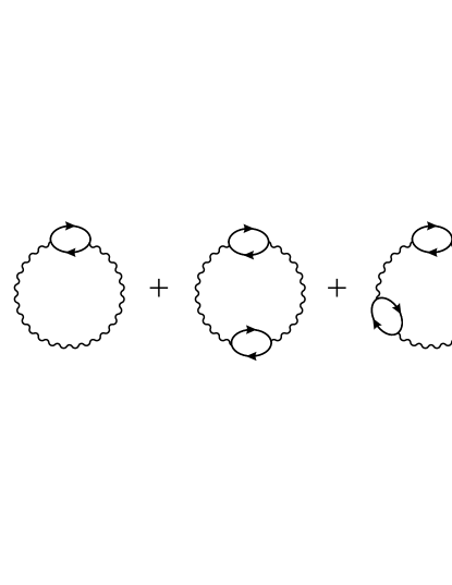
Figure 1: The Feynman diagram for the Coulomb interaction contribution to the ground state energy within RPA. The circles are polarization bubbles, the wiggly lines are the bare Coulomb interaction, and the solid lines the noninteracting electron Green’s function.

Note that the distribution function enters into the expression of ground state energy $E_{G}$ through the noninteracting Green’s function

$$G^{(0)}({\bf k},\omega)={n_{\bf k}\over\omega-\xi_{\bf k}-i\eta}+{1-n_{\bf k}\over\omega-\xi_{\bf k}+i\eta},$$ (2)

where $\xi_{\bf k}=k^{2}/(2m)-E_{F}$ is the non-interacting electron energy with $E_{F}$ as the Fermi energy or the non-interacting chemical potential, and $\eta$ is an infinitesimal positive number. It is easy to obtain the variational derivative of the Green’s function as

$${\delta\over\delta n_{\bf k}}G^{(0)}({\bf q},\omega)=2\pi i\delta(\omega-\xi_{\bf k})\delta({\bf k-q}).$$ (3)

Graphically, taking the $n_{\bf k}$ variational derivative of a quantity simply means cutting one solid line of the Feynman diagram and taking the external momentum and frequency to be on-shell (i.e. $\omega=\xi_{\bf k}$). We show the corresponding Feynman diagram for the self-energy in Fig. 2. We emphasize that the RPA or the ring-diagram approximation (which is appropriate for electron liquids interacting with the long-range Coulomb interaction) as shown in Fig. 1 necessarily implies that the on-shell self-energy approximation is used for calculating the quasiparticle energy dispersion (Fig. 2) since all energy and momenta in Fig. 1 correspond to the noninteracting system.

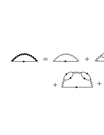
Figure 2: The Feynman diagram for the self-energy within RPA. The thick wiggly line denotes the dynamically screened Coulomb interaction.

The second order derivative of the total ground energy is referred to as Landau’s interaction function:

$$f({\bf k},{\bf k^{\prime}})={\partial^{2}E_{G}\over\partial n_{\bf k}\partial n_{\bf k}}.$$ (4)

The Feynman diagram for the interaction function within RPA is shown in Fig. 3.

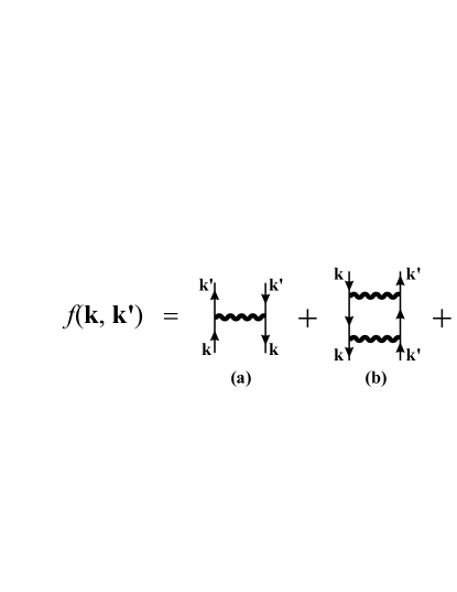
Figure 3: The Feynman diagram for the Landau interaction function $f({\bf k},{\bf k^{\prime}})$ within RPA.

Landau’s interaction function (4) determines renormalization of the effective mass $m^{*}$ relative to the bare mass $m$

$${1\over m^{*}}={1\over m}-C\int f(\theta)\cos\theta\,do,$$ (5)

where $\theta$ is the angle between ${\bf k}$ and ${\bf k^{\prime}}$, $do$ the element of solid angle along ${\bf k^{\prime}}$ in 3D and $d\theta$ in 2D, and $C=k_{F}/(2\pi)^{3}$ in 3D and $C=1/(2\pi)^{2}$ in 2D.

The contribution (a) in Fig. 3 to Landau’s interaction function is nothing but the static screened Coulomb interaction

$$f_{a}(q)=-\frac{2\pi e^{2}}{q+\kappa}\quad\mbox{in 2D},\quad f_{a}(q)=-\frac{4\pi e^{2}}{q^{2}+\kappa^{2}}\quad\mbox{in 3D},$$ (6)

where $q=|{\bf k}-{\bf k^{\prime}}|$ is momentum transfer between the two interacting electrons, and $\kappa$ is the appropriate inverse screening length. The minus sign in Eq. (6) reflects the exchange character of the Coulomb interaction between two fermions. Because the amplitude of $f_{a}(q)$, given by Eq. (6), is maximal at $q=0$, i.e. at $\theta=0$, where $\cos\theta>0$, it produces a positive contribution to the right-hand side of Eq. (5) and tends to decrease $m^{*}$. Because the first term $f_{a}$ dominates over the other two terms $f_{b}$ and $f_{c}$ in Fig. 3 at small $r_{s}$, thus $m^{*}<m$ at small $r_{s}$ (see Fig. 6 of Ref. Rice, 1965).

However, the sum of the $f_{b}$ and $f_{c}$ terms in Fig. 3 has the same sign as $f_{a}$ in Eq. (6), but its maximal amplitude is achieved at ${\bf k}=-{\bf k^{\prime}}$, i.e. at $\theta=\pi$, where $\cos\theta<0$ (see Fig. 10 of Ref. Rice, 1965). Thus, $f_{b}$ and $f_{c}$ produce a negative contribution to the right-hand side of Eq. (5) and tend to increase $m^{*}$. Because the strength of the $f_{b}$ and $f_{c}$ terms (“two-plasmon exchange”) increases relative to $f_{a}$ (“one-plasmon exchange”) with the increase of $r_{s}$, the effective mass $m^{*}$ starts to increase and becomes greater than $m$. This effect was already seen in Fig. 6 of Ref. Rice, 1965. However, the numerical calculations of Ref. Rice, 1965 stopped at a moderate $r_{s}\sim 4$. In Ref. Zhang and Das Sarma, a, essentially the same calculations were extended to greater $r_{s}$, and divergence of $m^{*}$ was found. The divergence of $m^{*}$ occurs at the point where the interaction term in the right-hand side of Eq. (5) becomes equal to the bare term.

An alternative, but in some sense similar scenario of mass divergence was proposed in Ref. Khodel et al., based on a phenomenological assumption that $f(q)$ has maximal amplitude at $q\sim 2k_{F}$, where $\cos\theta<0$, due to proximity to a density-wave instability.

II.2 Dielectric function

The key quantity in evaluating the self-energy is the dynamically screened Coulomb interaction $u({\bf q},\omega)\equiv v_{q}/\epsilon({\bf q},\omega)$, where $v_{q}$ is the Coulomb interaction in momentum space and $\epsilon({\bf q},\omega)$ is the dynamical dielectric function Abrikosov et al. ; Rice (1965); Hedin ; Hubbard . The Coulomb interaction is given by $v_{q}=2\pi e^{2}/q$ (2D) and $4\pi e^{2}/q^{2}$ (3D) with $q\equiv|{\bf q}|$ being the appropriate 2D or 3D momentum. The dielectric function is given by the infinite geometric series of the noninteracting ring diagrams where each ring is just the noninteracting electron polarizability. The 2D and 3D dielectric functions $\epsilon(q,\omega)=1-v_{q}\Pi(q,\omega)$ are given in Stern Stern (1967) and Linhard Lindhard (1954) respectively, where $\Pi(q,\omega)$ is the polarizability, which can be denoted as one ring or bubble as in Fig. 1 and Fig. 2.

In actual calculations it is conventional to express all the expressions in terms of the dimensionless units $r_{s}$. The relation between $r_{s}$ and Fermi vector is $r_{s}=1/(\alpha k_{F}a_{B})$, where $\alpha^{(2D)}=1/2$ and $\alpha^{(3D)}=(9\pi/2)^{-1/3}$. For completeness we write down the expression of 2D and 3D $\epsilon(q,\omega)$ in the units of $2k_{F}=4E_{F}=2m=1$, i.e. we use $x=q/(2k_{F})$ to denote momentum and $u=\omega/(4E_{F})$ to denote energy. For 2D $u>0$ case we have:

$$\!\!\!\!\!\!\mbox{Re}~{}\epsilon(x,u)=1+{\alpha r_{s}\over 2x}\Bigg{\{}1$$

$$-{1\over 2x^{2}}\mbox{Sign}(x^{2}-u)\Theta[(u-x^{2})^{2}-x^{2}]\sqrt{(u-x^{2})^{2}-x^{2}}$$

$$-{1\over 2x^{2}}\mbox{Sign}(x^{2}+u)\Theta[(u+x^{2})^{2}-x^{2}]\sqrt{(u+x^{2})^{2}-x^{2}}\Bigg{\}},$$

$$\!\!\!\!\!\!\mbox{Im}~{}\epsilon(x,u)={\alpha r_{s}\over 4x^{3}}\Bigg{\{}\Theta[x^{2}-(u-x^{2})^{2}]\sqrt{x^{2}-(u-x^{2})^{2}}$$

$$-\Theta[x^{2}-(u+x^{2})^{2}]\sqrt{x^{2}-(u+x^{2})^{2}}\Bigg{\}},$$

$$\!\!\!\!\!\!\epsilon(x,iu)=1+{\alpha r_{s}\over 2x}\Bigg{[}1$$

$$-{1\over\sqrt{2}x^{2}}\sqrt{x^{4}-x^{2}-u+\sqrt{(x^{4}-x^{2}-u)^{2}+4u^{2}x^{4}}}\Bigg{]},$$ (7)

where $\Theta(x)=1$ when $x>0$ and $0$ otherwise. For 3D $u>0$ case we have

$$\mbox{Re}~{}\epsilon(x,u)=1 + {\alpha r_{s}\over\pi 4x^{2}}\Bigg{\{}1$$

$$+ {1\over 4x^{3}}[x^{2}-(x^{2}+u)^{2}]\ln\left|{q^{2}+q+u\over q^{2}-q+u}\right|$$

$$+ {1\over 4x^{3}}[x^{2}-(x^{2}-u)^{2}]\ln\left|{q^{2}+q-u\over q^{2}-q-u}\right|\Bigg{\}}$$

$$\mbox{Im}~{}\epsilon(x,u)=\left\{\begin{array}[]{ll}{\alpha r_{s}u\over 2x^{3}}&(x-x^{2}>u>0)\\ \\ {\alpha r_{s}\over 8x^{5}}[x^{2}-(x^{2}-u)^{2}]&(x^{2}+x>u>|x^{2}-x|)\\ \\ 0&(\mbox{Otherwise})\end{array}\right.$$ (13)

$$\epsilon(x,iu)=1 + {\alpha r_{s}\over\pi 4x^{2}}\Bigg{\{}1$$ (14)

$$+ {1\over 4x^{3}}[x^{2}-x^{4}+u^{2}]\ln\left[{(q^{2}+q)^{2}+u^{2}\over(q^{2}-q)^{2}+u^{2}}\right]$$

$$+ {u\over x}\left[\arctan({u\over q^{2}+q})-\arctan({u\over q^{2}-q})\right]\Bigg{\}}.$$

In both 2D and 3D we have the relation $\epsilon(x,-u)=\epsilon^{*}(x,u)$ (complex conjugate) and $\epsilon(x,-iu)=\epsilon(x,iu)$.

II.3 Quasiparticle self-energy

The one-loop self-energy (Fig. 2) at zero temperature can be written as

$$\Sigma({\bf k},\omega) = -\int{d^{d}q\over(2\pi)^{d}}\int{d\nu\over 2\pi i}{v_{q}\over\epsilon({\bf q},\nu)}$$ (15)

$$~{}~{}~{}~{}~{}~{}~{}~{}\cdot G^{(0)}({\bf k+q},\omega+\nu).$$

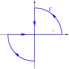
Figure 4: Contour in the frequency $\nu$ plane. The cross denotes the possible position of the pole of Green’s function.

Due to the difficulty with the principal value integration and singularities of $1/\epsilon({\bf k},\omega)$ along the real axis in Eq. (15), it is advantageous to follow the standard procedure and deform the frequency integration from the real axis to the imaginary axis. After choosing the contour of frequency integration as in Fig. 4, we consider the integration

$$\oint_{\Gamma}{d\nu\over 2\pi i}w({\bf q},\nu)G_{0}({\bf q}+{\bf k},\nu+\omega),$$ (16)

where $w({\bf q},\nu)$ is any complex function that is analytic in the upper and lower half of the complex plane which satisfies the condition that $w({\bf q},\nu)\to 0$ as $|\nu|\to\infty$. On the one hand, (16) equals the integration of the integrand along real and imaginary axes since the integration along the curved part of the contour $\Gamma$ (Fig. 4) vanishes. On the other hand, (16) equals the residue due to the pole of Green’s function

$$- [1-n_{F}(\xi_{{\bf q}+{\bf k}})]\Theta(\omega-\xi_{{\bf q}+{\bf k}})w({\bf q},\xi_{{\bf q}+{\bf k}}-\omega-i\eta)$$ (17)

$$+ n_{F}(\xi_{{\bf q}+{\bf k}})\Theta(\xi_{{\bf q}+{\bf k}}-\omega)w({\bf q},\xi_{{\bf q}+{\bf k}}-\omega+i\eta),$$

where $n_{F}(x)$ is the Fermi distribution function (At $T=0$ $n_{F}(x)=1$ for $x<0$ and $0$ otherwise). Now by setting

$$w({\bf k},\omega)={1\over\epsilon({\bf k},\omega)}-1,$$ (18)

we have

$$\!\!\!\!\!\!\!\!\!\!\!\!\Sigma({\bf k},\omega)=-\int{d^{d}q\over(2\pi)^{d}}v_{q}n_{F}(\xi_{{\bf q}+{\bf k}})$$ (20)

$$-\int{d^{d}q\over(2\pi)^{d}}\int{d\nu\over 2\pi i}v_{q}w({\bf q},\nu)G_{0}({\bf q}+{\bf k},\nu+\omega)$$

$$= -\int{d^{d}q\over(2\pi)^{d}}v_{q}n_{F}(\xi_{{\bf q}+{\bf k}})$$

$$-\int{d^{d}q\over(2\pi)^{d}}\Big{\{}-[1-n_{F}(\xi_{{\bf q}+{\bf k}})]$$

$$~{}~{}~{}\cdot\Theta(\omega-\xi_{{\bf q}+{\bf k}})w({\bf q},\xi_{{\bf q}+{\bf k}}-\omega-i\eta)$$

$$~{}~{}~{}~{}+n_{F}(\xi_{{\bf q}+{\bf k}})\Theta(\xi_{{\bf q}+{\bf k}}-\omega)w({\bf q},\xi_{{\bf q}+{\bf k}}-\omega+i\eta)\Big{\}}$$

$$-\int{d^{d}q\over(2\pi)^{d}}\int{d\nu\over 2\pi}{w({\bf q},i\nu)\over i\nu+\omega-\xi_{{\bf q}+{\bf k}}}.$$

Note that the first term in Eq. (20), usually named the exchange part, is a singular term when temperature is zero. Thus we rewrite the first and the second term so that they are well defined. Real and imaginary parts of the self-energy $\Sigma({\bf k},\omega)=\Sigma^{\prime}({\bf k},\omega)+i\Sigma^{\prime\prime}({\bf k},\omega)$ can then be written as

$$\!\!\!\!\!\!\!\!\!\!\Sigma^{\prime}({\bf k},\omega)=-\int{d^{d}q\over(2\pi)^{d}}v_{q}\Theta(2m\omega+k_{F}^{2}-|{\bf q-k}|^{2})$$

$$+\int{d^{d}q\over(2\pi)^{d}}v_{q}\mbox{Re}~{}{1\over\epsilon({\bf q},\xi_{\bf q-k}-\omega)}$$

$$~{}~{}~{}\cdot\Big{[}\Theta(2m\omega+k_{F}^{2}-|{\bf q-k}|^{2})-\Theta(k_{F}^{2}-|{\bf q-k}|^{2})\Big{]}$$

$$-\int{d^{d}q\over(2\pi)^{d}}\int{d\nu\over 2\pi}v_{q}\left[{1\over\epsilon({\bf q},i\nu)}-1\right]{1\over i\nu+\omega-\xi_{{\bf q}+{\bf k}}},$$ (21)

$$\Sigma^{\prime\prime}({\bf k},\omega)=\int{d^{d}q\over(2\pi)^{d}}v_{q}\mbox{Im}~{}{1\over\epsilon({\bf q},\xi_{\bf q-k}-\omega)}$$

$$~{}~{}~{}\cdot\Big{[}\Theta(2m\omega+k_{F}^{2}-|{\bf q-k}|^{2})-\Theta(k_{F}^{2}-|{\bf q-k}|^{2})\Big{]}.$$ (22)

To be consistent with our leading-order one-loop approximation in the dynamically screened Coulomb interaction (Figs. 1 and 2) we should calculate the self-energy only within the on-shell approximation Zhang and Das Sarma (a); Rice (1965) instead of solving the full Dyson’s equation. After putting $\omega=\xi_{\bf k}$ (i.e. the on-shell approximation), we express the above equations in terms of $r_{s}$, while using $2k_{F}$ as the unit of wave-vector, and $4E_{F}$ as the energy unit. For 2D real part of self-energy $\Sigma_{\bf k}\equiv\Sigma({\bf k},\omega=\xi_{\bf k})$ we obtain

$$\!\!\!\!\!\!\!\!\!\!{\Sigma^{\prime}_{\bf k}\over 4E_{F}}=-{2\alpha r_{s}\over\pi}y$$

$$+{\alpha r_{s}\over\pi}\int_{1/2}^{y}dx\int_{0}^{\pi}d\theta{x\over\sqrt{x^{2}-2xy\cos(\theta)+y^{2}}}$$

$$~{}~{}~{}\cdot\mbox{Re}~{}{1\over\epsilon\left(\sqrt{x^{2}-2xy\cos(\theta)+y^{2}},x^{2}-y^{2}\right)}$$

$$-{\alpha r_{s}\over\sqrt{2}\pi}\int dx\int du\left[{1\over\epsilon({\bf x},ixu)}-1\right]$$

$$\cdot{\sqrt{(x^{2}-u^{2}-4y^{2})+\sqrt{(x^{2}-u^{2}-4y^{2})^{2}+4y^{2}u^{2}}}\over\sqrt{(x^{2}-u^{2}-4y^{2})^{2}+4x^{2}u^{2}}},$$ (23)

where ${\bf y}={\bf k}/(2k_{F})$. Similarly for 3D we have

$$\!\!\!\!\!\!\!\!\!\!{\Sigma^{\prime}_{\bf k}\over 4E_{F}}=-{\alpha r_{s}\over\pi}y$$

$$+{\alpha r_{s}\over\pi}\int_{1/2}^{y}dx\int_{0}^{\pi}d\theta{x^{2}\over x^{2}-2xy\cos(\theta)+y^{2}}$$

$$~{}~{}~{}\cdot\mbox{Re}~{}{1\over\epsilon\left(\sqrt{x^{2}-2xy\cos(\theta)+y^{2}},x^{2}-y^{2}\right)}$$

$$-{\alpha r_{s}\over 4\pi^{2}y}\int_{0}^{\infty}dx\int_{0}^{\infty}du\left[{1\over\epsilon({\bf x},ixu)}-1\right]$$

$$~{}~{}~{}\cdot\ln\left[{(2y-x)^{2}+u^{2}\over(2y+x)^{2}+u^{2}}\right].$$ (24)

The 2D imaginary self-energy can be written down as,

$${\Sigma^{\prime\prime}_{\bf k}\over 4E_{F}} = {\alpha r_{s}\over\pi}\int_{1/2}^{y}dx\int_{0}^{\pi}d\theta{x\over\sqrt{x^{2}-2xy\cos(\theta)+y^{2}}}$$ (25)

$$\cdot\mbox{Im}~{}{1\over\epsilon\left(\sqrt{x^{2}-2xy\cos(\theta)+y^{2}},x^{2}-y^{2}\right)},$$

and for 3D imaginary quasiparticle self-energy we have

$${\Sigma^{\prime\prime}_{\bf k}\over 4E_{F}} = {\alpha r_{s}\over\pi}\int_{1/2}^{y}dx\int_{0}^{\pi}d\theta{x^{2}\over x^{2}-2xy\cos(\theta)+y^{2}}$$ (26)

$$\cdot\mbox{Im}~{}{1\over\epsilon\left(\sqrt{x^{2}-2xy\cos(\theta)+y^{2}},x^{2}-y^{2}\right)}.$$

II.4 Quasiparticle energy dispersion and damping

The quasiparticle dispersion is given simply by adding the on-shell real self-energy to the noninteracting electron energy

$$E_{\bf k}\equiv\xi_{\bf k}+\Sigma^{\prime}_{\bf k}.$$ (27)

The quasiparticle damping rate, which is non-zero away from the Fermi surface $k\neq k_{F}$, is given by the on-shell imaginary part of the self-energy

$$\Gamma_{\bf k}=\left|\mbox{Im}~{}\Sigma({\bf k},\xi_{\bf k})\right|=\Sigma^{\prime\prime}_{\bf k}.$$ (28)

The renormalized quasiparticle effective mass is given by

$${1\over m^{*}({\bf k})}={1\over k}{dE_{\bf k}\over dk}.$$ (29)

It is clear that we get $m^{*}\equiv m$, the constant bare electron mass, if we use the noninteracting energy $\xi_{\bf k}=k^{2}/(2m)$ for $E_{\bf k}$, i.e. if we put the self-energy to be zero. Putting $k=k_{F}$ one gets the quasiparticle effective mass at the Fermi surface, as calculated in Ref. Zhang and Das Sarma, a. For an arbitrary $k\neq k_{F}$, $m({\bf k})$ defines the dispersing quasiparticle mass, i.e. the generalized wavevector-dependent quasiparticle effective mass.

III Results

In this section we present our calculated results showing the quasiparticle energy dispersion for both 2D and 3D electron systems with long range Coulomb interactions. The dispersion instability at large $r_{s}$ will be obvious in these results.

In Fig. 5 we plot the calculated quasiparticle energy as a function of momentum for different $r_{s}$ values in a 2D system. It is clear that the quasiparticle effective mass ($m^{*}=k_{F}(dE_{k}/dk)^{-1}|_{k=k_{F}}$) diverges at some low density at critical $r_{s}$ value $r_{s}^{*}\sim 18$. As $r_{s}$ increases, not only the energy dispersion of the quasiparticles around Fermi surface becomes flatter (i.e. relatively independent of momentum), but the dispersion in the whole momentum space is fundamentally changed. The quasiparticle energy dispersion in a 3D electron system is presented in Fig. 6, showing the dispersion “flattening” for a range of wavevector $k$ at a critical $r_{s}^{*}\sim 50$.

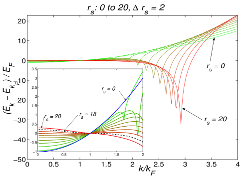
Figure 5: (Color online) 2D quasiparticle energy as a function of momentum at $r_{s}$ values ranging from $0$ to $20$. Inset: zoom-in of the spectrum with $k/k_{F}<2$. The dashed line indicate the $r_{s}$ value at which the effective mass at the Fermi surface shows divergence ($r_{s}^{*}\sim 18$).

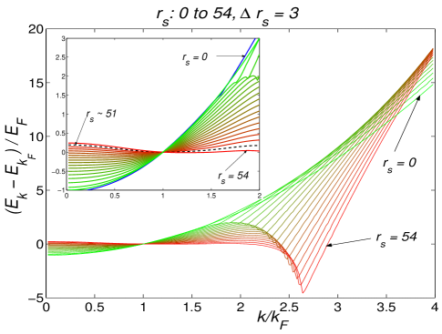
Figure 6: (Color online) 3D quasiparticle energy as a function of momentum at $r_{s}$ values ranging from $0$ to $54$. Inset: zoom-in of the spectrum with $k/k_{F}<2$. The dashed line indicate the $r_{s}$ value at which the effective mass at the Fermi surface shows divergence $r_{s}^{*}\sim 50$.

An obvious common feature of both 2D and 3D quasiparticle energy dispersion is that at some large momentum, the dispersion shows a kink, which indicates the plasmon-resonance. This is the threshold wavevector at which the quasiparticle can emit plasmons obeying energy-momentum conservation Jalabert and Das Sarma . This plasmon-emission-induced kink in $E_{\bf k}$ for $k>k_{F}$ occurs at all $r_{s}$, with the threshold wavevector $k_{th}$ being $r_{s}$-dependent. As $r_{s}$ increases, this resonance feature becomes stronger. To further substantiate the connection between the dispersion (and the associated effective mass divergence) and the plasmon resonance we show in Figs. 7 (2D) and 8 (3D) our calculated quasiparticle energy dispersion together with the calculated quasiparticle damping $\Gamma_{\bf k}\equiv Im\Sigma({\bf k},\xi_{\bf k})$. It is obvious from Figs. 7 and 8 that the “dip” (at $k>k_{F}$) in the quasiparticle dispersion occurs precisely at the plasmon emission threshold wavevector Jalabert and Das Sarma . The energy-momentum conservation makes it impossible Jalabert and Das Sarma for plasmon emission by quasiparticles to happen below the threshold momentum $k_{th}$. Since the real and imaginary parts of the electron self-energy function are connected through the Kramers-Kronig causality relations, the plasmon emission threshold in the quasiparticle damping (i.e. $\mbox{Im}\Sigma$) shows up as a kink in the quasiparticle dispersion (i.e. $\mbox{Re}\Sigma$). This kink or the dip in the dispersion indicates a nonlinear instability of the quasiparticles over a finite range of momentum since the quasiparticle velocity becomes manifestly negative for $k\lesssim k_{th}$ where the dispersion is locally inverted. With increasing $r_{s}$, interaction effects become stronger and the plasmon-emission-induced kink also becomes deeper indicating a progressively stronger (with increasing $r_{s}$) nonlinear instability around $k_{th}$. The plasmon emission threshold $k_{th}(>k_{F})$ is given by the solution of the following transcendental equation:

$$\max_{k_{F}<q<k_{th}}\epsilon(k_{th}-q,{k^{2}_{th}\over 2m}-{q^{2}\over 2m})=0.$$ (30)

Below we discuss the (partial) connection between the plasmon emission phenomenon (leading to the ‘kink’ in the quasiparticle dispersion at the plasmon resonance momentum $k_{th}$) and the dispersion instability, which is quite apparent in Figs. 5, 6, 7, 8, and at the same time emphasize some subtle features about this connection, which point to the qualitative nature of this connection.

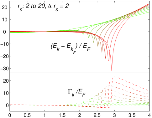
Figure 7: (Color online) 2D real and imaginary quasiparticle energy as a function of momentum at $r_{s}$ values ranging from $2$ to $20$.

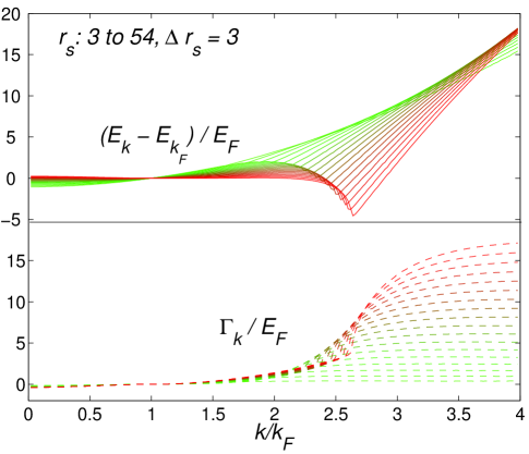
Figure 8: (Color online) 3D real and imaginary quasiparticle energy as a function of momentum at $r_{s}$ values ranging from $3$ to $54$.

A closer examination of the energy dispersion (see Figs. 5 and 6) provides interesting insights. Here we focus on the momentum region where the dispersion shows instability. The divergence of the effective mass (i.e. the inverse slope of the energy spectrum) for quasiparticles at different wavevecter (not just at the Fermi surface) is a good indication of these instabilities (also see Figs. 9 and 10). Due to the presence of the plasmon resonance which we described in the last paragraph, one effective mass divergence happens at momentum (which we call the upper instability momentum $k_{h}^{*}$) slightly smaller than the threshold resonance momentum ($k_{th}$) for both 2D and 3D systems, i.e. $m^{*}(k)\to\infty$ as $k\to k_{h}^{*}$. The energy dispersion reaches a local maximum when $k=k_{h}^{*}$. As we mentioned, this feature exists for all $r_{s}$ values. However, for low electron density, this is not the only instability feature that occurs. In fact in both 2D and 3D, for $r_{s}$ above a certain value, a quasihole instability emerges at a smaller momentum, which we call the lower instability momentum $k_{l}^{*}$. The energy dispersion reaches local minimum when $k=k_{l}^{*}$, and $m^{*}(k)\to\infty$ as $k\to k_{l}^{*}$. In other words, the slope of the energy dispersion is negative in the region $k<k_{l}^{*}$, positive for $k_{l}^{*}<k<k_{h}^{*}$, negative for $k_{h}^{*}<k<k_{th}$, and then positive for $k>k_{th}$. So it is clear that, for big enough $r_{s}$ (but still smaller than $r_{s}^{*}$), there are two instability regions $k<k_{l}^{*}$ and $k_{h}^{*}<k<k_{th}$ away from Fermi surface ($k_{l}^{*}<k_{F}<k_{h}^{*}$), where the momentum dependent effective mass is negative. (For very small $r_{s}$ we only have the quasiparticle instability region $k_{h}^{*}<k<k_{th}$.) We note that while the quasiparticle dispersion instability at $k^{*}_{h}\lesssim k_{th}$ is induced by plasmon emission due to the obvious connection between $k_{h}^{*}$ and $k_{th}$, no such simple explanation seems to apply to the corresponding quasihole instability at $k<k_{l}^{*}$.

For $r_{s}<r_{s}^{*}$, the lower and upper instability regions remain below and above Fermi surface, and therefore are not of any particular significance since the quasiparticle damping ($\Gamma_{\bf k}\equiv\mbox{Im}\Sigma({\bf k},\xi_{\bf k})$) is finite. As $r_{s}$ increases, both of these two regions grow larger: $k_{l}^{*}$ increases, $k_{h}^{*}$ decreases, and $k_{th}$ increases with increasing $r_{s}$. If one (or both) of these two instability regions reaches the Fermi surface, the effective mass on the Fermi surface diverges. This is indeed what happens except that the details are slightly different depending on the system dimensionality (2D or 3D). In 2D, as $r_{s}\to r_{s}^{*}$, both instability regions reach $k_{F}$ at the same time, whereas in 3D it appears that the quasihole instability reaches $k_{F}$ first at $r_{s}=r_{s}^{*}$. The difference between 2D and 3D results arises from the very different density of states in the two cases.

For 2D, when $r_{s}\sim 10$, $k_{l}^{*}$ starts out at zero momentum, and as $r_{s}$ increases, $k_{l}^{*}$ increases and at the same time $k_{h}^{*}$ decreases. As $r_{s}$ reaches the critical value $r_{s}^{*}\sim 18$, $k_{l}^{*}=k_{h}^{*}=k_{F}$, which is the critical value at which the effective mass at the Fermi surface diverges. When $r_{s}>r_{s}^{*}$, there is no effective mass divergence in the whole momentum space, and the dispersion is inverted for all $k<k_{th}$. The 3D case is a little different. As $r_{s}\sim 28$, $k_{l}^{*}$ first emerges at zero momentum, and keeps increasing as $r_{s}$ increases while $k_{h}^{*}$ decreases. As $r_{s}$ reaches the value $r_{s}^{*}\sim 50$, $k_{l}^{*}=k_{F}$, and the effective mass at the Fermi surface diverges. However at this $r_{s}$, another effective mass divergence happens at $k_{h}^{*}>k_{F}$. Only when $r_{s}$ increases to more than $58$, $k_{l}^{*}$ and $k_{h}^{*}$ meet each other at around $1.6k_{F}$, after which the effective mass does not diverge in the whole momentum space.

Because it is difficult to visually locate the local maximum and minimum in the energy dispersion, we show in Figs. 9 and  10 our calculated momentum-dependent quasiparticle effective mass $m^{*}({\bf k})=[k^{-1}dE_{\bf k}/dk]^{-1}$. Of course, the concept of a quasiparticle effective mass far away from the Fermi surface is not particularly meaningful since these quasiparticles are necessarily highly damped with short lifetimes. Nevertheless it is important to realize that the effective mass divergence initially develops for $r_{s}<r_{s}^{*}$ (i.e. at densities much larger than the critical density for the effective mass divergence at the Fermi surface) at wavevectors $k_{h}^{*}>k_{F}$ and $k_{l}^{*}<k_{F}$ far away from the Fermi surface. Eventually at $r_{s}=r_{s}^{*}$ the effective mass divergence reaches $k_{F}$, becoming at the same time a dispersion instability where the quasiparticle dispersion $E_{\bf k}$ essentially becomes almost flat all around $k_{F}$, implying $m({\bf k})$ to be divergent at the Fermi surface. This approximate “band-flattening”, i.e. $E_{\bf k}$ approximately independent of ${\bf k}$, for large enough $r_{s}$ values is also apparent in Figs. 5, 6, 7, 8.

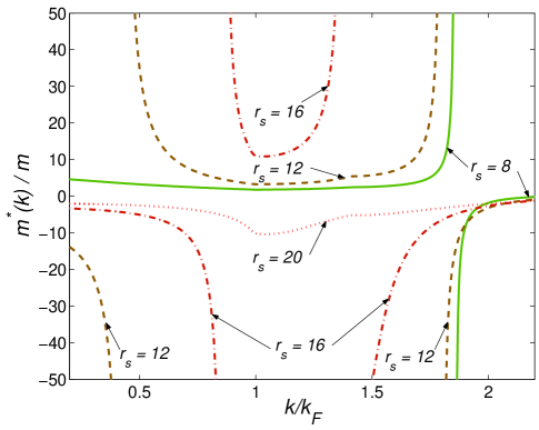
Figure 9: (Color online) Momentum dependent 2D quasiparticle effective mass for $r_{s}=8,12,16,20$.

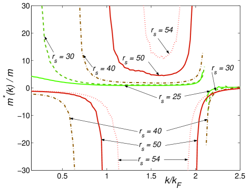
Figure 10: (Color online) Momentum dependent 3D quasiparticle effective mass for $r_{s}=25,30,40,50,54$.

Before concluding this section we mention that the critical $r_{s}^{*}$ for the effective mass divergence ($18$ for 2D and $50$ for 3D) obtained in this work is slightly larger than that obtained in Ref. Zhang and Das Sarma, a ($16$ in 2D and $48$ in 3D) since the current work considers spinless (or equivalently, spin-polarized) electrons whereas Ref. Zhang and Das Sarma, a dealt with a paramagnetic electron system with a spin degeneracy of $2$. It is interesting that $r_{s}^{*}$ shows only a weak dependence on the spin-polarization properties of the electron liquid. We believe that, while the basic mass divergence and band flattening phenomena are generic phenomena in strongly interacting electron liquids, the precise value of $r_{s}^{*}$ must depend on the approximation scheme involved, and it is likely that the “correct” $r_{s}^{*}$ is larger than that obtained within RPA. Our reason for using spinless electrons in our calculation is that within RPA the electron system undergoes a ferromagnetic transition Zhang and Das Sarma (b) of either Stoner or Bloch type to full spin polarization at a critical $r_{s}$ value which is lower than $r_{s}^{*}$, the critical $r_{s}$ for the mass divergence, and therefore it is more appropriate to carry out the dispersion-instability/mass-divergence calculation for a fully spin-polarized electron system as we do in the current work. We also notice that previous theoretical works Rajagopal et al. (1978); Ortiz et al. (1999) predicted possible partial spin-polarized ground state in 3D electron systems. We do not consider this effect in our calculation because within the same approximation scheme as in the present work, we find Zhang and Das Sarma (b) that in 3D electron systems, the densities of the partial spin-polarization region are much higher than the density that corresponds to the divergence of effective mass, and therefore partial spin-polarization has no effect on the dispersion instability. Partial spin-polarization does not occur in 2D systems Rajagopal et al. (1978), and thus this issue does not arise for our 2D calculations.

IV Discussion and conclusion

We show in this paper that the standard (and widely used) ring diagram approximation (RPA) self-energy calculation leads to a quasiparticle dispersion instability in the strongly interacting electron liquid (both 2D and 3D) at a low critical density – the quasiparticle dispersion becomes almost “flat” around $k_{F}$ for $r_{s}=r_{s}^{*}$ and beyond the critical point, for $r_{s}>r_{s}^{*}$, the quasiparticle effective velocity becomes negative implying an instability. The band flattening phenomenon is similar to that envisioned by Khodel and Shaginyan Khodel and Shaginyan (1990) in a different context some years ago. We have also identified a physical mechanism leading to the dispersion instability and the associated effective mass divergence. We find that it arises partially from plasmon (or collective mode) emission by the quasiparticles – in some sense, the “recoil” associated with strong plasmon emission slows down the quasiparticles, eventually effectively “stopping” it, leading to the mass divergence and band flattening. We emphasize however, that the plasmon emission and recoil mechanism is at best a partial physical mechanism for the dispersion instability – it plays a crucial role, but is not the whole story.

Two important questions immediately arise in the context of our theoretical findings: (1) What does the dispersion instability signify or imply? (2) What, if any, are its experimental implications and consequences? We cannot answer either of these questions definitively. But we can speculate some possibilities. Since the answer to the second question obviously depends on the answer to the first question, we first discuss some possible answers to the first question.

The meaning or implication of the dispersion instability associated with the effective mass divergence and the quasiparticle band flattening has earlier been discussed in the literature. Two of us have earlier speculated Zhang and Das Sarma (a) that the effective mass divergence is essentially a continuum version of the Mott transition as envisioned, for example, in the Brinkman-Rice scenario Brinkman and Rice (1970). Such a Brinkman-Rice Mott transition scenario had earlier been invoked Vollhardt (1984) in the context of the “almost localization” phenomenon in normal He-3 where the short-ranged inter-fermion interaction (in contrast to the long-ranged Coulomb interaction we are considering) is known to lead to quasiparticle mass divergence in the strongly interacting regime (which curiously happens at very high, rather than very low, densities in He-3 since the interaction is short-ranged in that system). Usually the continuum analog of the Mott transition in an electron liquid system is thought to be the Wigner crystallization transition, which, according to the best current quantum Monte Carlo (QMC) simulations, occur at a critical $r_{s}$ of $38$ (2D) and $90$ (3D). It is entirely possible that the effective mass divergence and the band flattening we find within RPA is the precursor to (or perhaps the RPA signature for) the Wigner transition, but we cannot prove or establish this speculation with any kind of theoretical arguments. It would be highly desirable in this context to carry out QMC calculations to study the dispersion instability, but QMC studies are reliable only for the true ground state properties, and may be quite inaccurate for effective mass calculations.

A second possibility, closely related to the Wigner crystallization transition discussed above, is that the dispersion instability is essentially a charge density wave instability Khodel et al. . This is not an absurd proposition given that the possibility of a density-driven charge density wave instability in a jellium electron liquid was originally discussed Overhauser (1978) by Overhauser more than forty years ago. We have therefore carefully analyzed the wavevector dependent contributions to the quasiparticle self-energy as well as calculated the Fermi liquid interaction function $f({\bf k},{\bf k^{\prime}})$ to see if there are any characteristic wavevectors which predominantly contribute to the dispersion instability. As should be obvious from our results, there are no characteristic wavevectors in the effective mass divergence phenomenon that we have discovered since it arises from a dispersion instability in which the whole dispersion is strongly affected and all wavevectors seem to be equivalent. The plasmon emission threshold wavevector $k_{th}$ seems to be special since the “seed” or “source” of our dispersion instability at least partially lies in the soft plasmon emission process, but we see no reason to associate $k_{th}$ with a characteristic charge density wave instability. Similarly, the upper ($k_{h}^{*}$) and the lower ($k_{l}^{*}$) critical wavevectors where the mass divergence first manifest itself (Figs. 9 and 10) could be characteristic charge density wave vectors but we have seen no theoretical indication of such a CDW instability, at least within our RPA theory.

Anther possibility that has been much discussed in the literature  Khodel and Shaginyan (1990, 1992); Nozieres (1992); Khveshchenko et al. (1993) is a superconducting or fermionic condensation instability associated with the quasiparticle energy degeneracy in the flat dispersion around $k_{F}$. Such a superconducting instability is entirely different from the usual Kohn-Luttinger superconducting instability (in some high angular momentum channel) that is known to exist (with an exponentially low superconducting transition temperature) in interacting electron liquids. In our problem of dynamically screened Coulomb interaction, such a superconducting instability could possibly arise from the exchange of virtual plasmons (i.e. plasmon-mediated superconductivity) since emission of real plasmons is an underlying mechanism for our dispersion instability. We have, in fact, little to add to the existing discussion in the literature Khodel and Shaginyan (1990, 1992); Nozieres (1992); Khveshchenko et al. (1993) on the issue of a superconducting instability in the context of the dispersion instability except to note that the transition temperature is likely to be rather low for such a superconducting state.

We note in this context that Nozieres carried out Nozieres (1992) a penetrating and trenchant analysis of the original band-flattening phenomenon introduced in Ref. Khodel and Shaginyan, 1990. While discussing the instability, Nozieres Nozieres (1992) was quite pessimistic about the theoretical possibility of such an instability existing in a realistic model that allows for screening. In fact, Nozieres concluded that “screening of a strong long range interaction is such that the instability threshold cannot be reached”. Our work shows that this conclusion of Ref. Nozieres, 1992 is, in fact, too pessimistic since our one-loop calculation is precisely an expansion in the dynamically screened long-range Coulomb interaction. Thus, the effective mass divergence can certainly occur even when screening of a strong long range interaction is explicitly incorporated in the theory in contrast to Nozieres’ conclusion in Ref. Nozieres, 1992.

A real theoretical concern is the possibility that the effective mass divergence (and the dispersion instability) is just an unfortunate artifact of our specific self-energy approximation, namely the single-loop (leading-order in dynamically screened interaction) RPA self-energy calculation. Although such a possibility can never be ruled out theoretically (short of an exact treatment of the strongly interacting electron liquid problem) we have argued Zhang and Das Sarma (a) elsewhere that this is unlikely to be the case here, i.e., there is very good reason to believe that the dispersion instability at a low electron density is a generic property of the strongly interacting electron liquid (but the actual value of $r_{s}$ depends on the approximation scheme). Without repeating the arguments already discussed in Ref. Zhang and Das Sarma, a, we point out that RPA (which is a self-consistent field approximation, not a perturbative expansion in $r_{s}$ although RPA does become exact in the high density $r_{s}\to 0$ limit) works well (as compared with experimental data) at metallic densities ($r_{s}\sim 3-6$) in 3D systems Abrikosov et al. and at very low densities ($r_{s}\sim 10-20$) in 2D electron systems Hwang and Sarma (2001). Second, the RPA prediction for a ferromagnetic instability in electron liquids turns out to be generically “correct”, i.e. the most accurate QMC calculations also predict ferromagnetic instabilities in 2D and 3D electron systems except that RPA underestimates the critical $r_{s}$ for the electron liquid ferromagnetic instability. This suggests that the RPA prediction for the dispersion instability is also likely to be generically correct. Third, the original dispersion instability, envisioned in Ref. Khodel and Shaginyan, 1990, used a toy model (involving a rather unrealistic long-range interaction) which is completely and fundamentally different from our dynamically screened Coulomb interaction model – the fact that two completely different interaction models arrive at very similar qualitative conclusions about the dispersion instability (both in 2D and 3D) is again strongly suggestive of the possible generic nature of the instability. Fourth (and perhaps the most important of all), there are no general theoretical arguments against such a dispersion instability, and therefore, if the interaction is strong enough (i.e. $r_{s}$ large enough), there is no theoretical reason for the instability not to occur. This point becomes even stronger in the context of the existence of such an effective mass divergence (“almost-localized Fermi liquid”) in normal He-3 interacting via the short-range interaction. We also note that, as shown in Ref. Zhang and Das Sarma, a, the quasiparticle effective mass divergence occurs in many-body approximations going beyond the RPA (e.g. the Hubbard approximation Hubbard ), and the same is obviously true for the dispersion instabilities. Thus the instability exists in self-energy calculations beyond the one-loop approximation.

Finally, we discuss the experimental implications of our results. First we note that the critical density ($r_{s}^{*}=18$ (2D); $50$ (3D)) involved in the dispersion instability is extremely low for meaningful experiments to be carried out in real systems. Also, our $T=0$ theory does not say much about the finite temperature situation where these experiments are necessarily carried out. In fact, the temperature scale at such low densities is likely to be small, and therefore one may have to go to unrealistically low temperatures to see any experimental consequences of the dispersion instability even if the instability is real. It is important to emphasize that our RPA values for critical $r_{s}^{*}$ are probably lower bounds on the true $r_{s}^{*}$ which is likely to be larger than $r_{s}^{*}=18$ (2D) and $50$ (3D).

With these caveats in mind, it is interesting to note that there have been several recent experimental claims of the observation Shashkin of quasiparticle effective mass divergence in Si MOSFET-based low-density interacting 2D electron system at $r_{s}\sim 10$. These claims are, however, quite controversial, and in more dilute 2D hole systems, where $r_{s}$ could reach as low as $20-30$, no such mass divergence has been reported. We believe that these recently reported effective mass divergence claims in Si MOSFETs are most likely not connected with the dispersion instability discussed in our work. This is particularly true in view of the fact that the reported effective mass divergence does not seem to be a dispersion instability, and furthermore, the experimental critical $r_{s}^{*}$ ($\sim 10$) is far too low compared with the theoretical finding ($\sim 18$). In fact, we expect our theoretical $r_{s}^{*}$ to be much lower than the RPA value ($r_{s}^{*}\sim 18$ in 2D) predicted in our work once quasi-2D finite width effects and many-body effects going beyond RPA are included in the theory. In addition, the semiclassical experimental technique of using Dingle fits to temperature-induced SdH amplitude decay Shashkin in extracting the quasiparticle effective mass is highly suspect in such a strongly interacting quantum system. The experiments claiming the effective mass divergence also completely ignored the strong temperature dependence Das Sarma et al. of the quasiparticle effective mass which certainly invalidates the semiclassical Dingle fitting procedure employed in the experiments in obtaining the quasiparticle effective mass. We therefore conclude that the experimental consequences of the dispersion instability in low-density interacting electron liquids remain an interesting open challenge for the future.

We acknowledge fruitful discussions with M. V. Zverev and V. A. Khodel. This work is supported by the US-ONR and NSF.

References

- Zhang and Das Sarma (a) Y. Zhang and S. Das Sarma, cond-mat/0312565. (Phys. Rev. B, in press).
- Khodel and Shaginyan (1990) V. A. Khodel and V. R. Shaginyan, JETP Lett. 51, 553 (1990).
- (3) A. A. Abrikosov, L. P. Gor’kov, and I. E. Dzyaloshinski, Methods of quantum field theory in statistical physics (Dover Publications, New York, 1963); G. D. Mahan, Many-particle physics (Plenum Press, New York, 1981); A. L. Fetter and J. D. Walecka, Quantum theory of many-particle systems (McGraw-Hill, San Francisco, 1971).
- Khodel and Shaginyan (1992) V. A. Khodel and V. R. Shaginyan, JETP Lett. 55, 110 (1992).
- Nozieres (1992) P. Nozieres, J. Phys. I France 2, 443 (1992).
- Khveshchenko et al. (1993) D. Khveshchenko, R. Hlubina, and T. M. Rice, Phys. Rev. B 48, 10766 (1993).
- Volovik (1991) G. E. Volovik, JETP Lett. 53, 222 (1991).
- Zverev et al. (1996) M. V. Zverev, V. A. Khodel, and V. R. Shaginyan, JETP 82, 567 (1996).
- Lidsky et al. (1998) D. Lidsky, J. Shiraishi, Y. Hatsugai, and M. Kohmoto, Phys. Rev. B 57, 1340 (1998).
- (10) V. A. Khodel, V. R. Shaginyan, and M. V. Zverev, JETP Lett. 65, 253 (1997); V. M. Yakovenko and V. A. Khodel, JETP Lett. 78, 298 (2003); V. M. Galitski and V. M. Khodel, cond-mat/0308203.
- Rice (1965) T. M. Rice, Ann. Phys. (N. Y.) 31, 100 (1965).
- (12) L. Hedin, Phys. Rev. 139 A796, (1965); L. Hedin and S. Lundqvist, Solid State Physics (Academic Press, New York and London).
- (13) J. Hubbard, Proc. Roy. Soc. A240, 539 (1957); A243, 336 (1957).
- Stern (1967) F. Stern, Phys. Rev. Lett. 18, 546 (1967).
- Lindhard (1954) J. Lindhard, Mat.-fys. Medd. 28, No. 8 (1954).
- (16) R. Jalabert and S. Das Sarma, Phys. Rev. B39, 5542 (1989); Phys. Rev. B40, 9723 (1989).
- Zhang and Das Sarma (b) Y. Zhang and S. Das Sarma, cond-mat/0408335; Ying Zhang and S. Das Sarma, unpublished.
- Rajagopal et al. (1978) A. K. Rajagopal, S. P. Singhal, M. Banerjee, and J. C. Kimball, Phys. Rev. B 17, 2262 (1978).
- Ortiz et al. (1999) G. Ortiz, M. Harris, and P. Ballone, Phys. Rev. Lett. 82, 5317 (1999).
- Brinkman and Rice (1970) W. F. Brinkman and T. M. Rice, Phys. Rev. B 2, 4302 (1970).
- Vollhardt (1984) D. Vollhardt, Rev. Mod. Phys. 56, 99 (1984).
- Overhauser (1978) A. W. Overhauser, Phys. Rev. B 18, 2884 (1978).
- Hwang and Sarma (2001) E. H. Hwang and S. D. Sarma, Phys. Rev. B 64, 165409 (2001).
- (24) A. Shashkin, cond-mat/0405556, and references therein.
- (25) S. Das Sarma, V. M. Galitski, and Y. Zhang, Phys. Rev. B69, 125334 (2004); Ying Zhang and S. Das Sarma, Phys. Rev. B70, 035104 (2004); V. M. Galitski and S. Das Sarma, Phys. Rev. B70, 035111 (2004); A. V. Chubukov and D. L. Maslov, Phys. Rev. B68, 155113 (2003).