Weak-coupling phase diagrams of bond-aligned and diagonal doped Hubbard ladders

Abstract

We study, using a perturbative renormalization group technique, the phase diagrams of bond-aligned and diagonal Hubbard ladders defined as sections of a square lattice with nearest-neighbor and next-nearest-neighbor hopping. We find that for not too large hole doping and small next-nearest-neighbor hopping the bond-aligned systems exhibit a fully spin-gapped phase while the diagonal systems remain gapless. Increasing the next-nearest-neighbor hopping typically leads to a decrease of the gap in the bond-aligned ladders, and to a transition into a gapped phase in the diagonal ladders. Embedding the ladders in an antiferromagnetic environment can lead to a reduction in the extent of the gapped phases. These findings may suggest a relation between the orientation of hole-rich stripes and superconductivity as observed in La_2-xSr_xCuO₄ .

I Introduction

There is a growing number of experiments which suggest that the existence of inhomogeneous electronic structures is a generic feature of the hole-doped high-temperature superconductors. Often these structures take the shape of quasi-one-dimensional hole-rich stripes running along various directions in the copper-oxygen planes [1]. The relevance of inhomogeneities in general and stripes in particular to the phenomenon of high-temperature superconductivity is presently far from being a settled issue.

Neutron-scattering experiments have produced clear evidence for a significant correlation between signatures of incommensurate spin excitations in La_2-xSr_xCuO₄ and the superconducting properties of this compound. Recently, it has been demonstrated [2] that such low-energy incommensurate spin excitations exist in the superconducting phase of La_2-xSr_xCuO₄ all the way up to its overdoped boundary at $x=0.28$, where they disappear simultaneously with superconductivity. On the underdoped side of the phase diagram static magnetic stripe signatures exist both in the insulating spin-glass phase [3, 4, 5] with $0.02\leq x\leq 0.05$ and in the underdoped superconductor [6, 7, 8] with $0.05\leq x\leq 0.12$. However, the transition from the insulator to the superconductor at $x=0.05$ is accompanied by a rotation of the stripe signal from the diagonal direction in the former to a bond-aligned signal in the latter. Moreover, angle resolved photoemission spectroscopy (ARPES) has revealed [9] an apparent coincidence between the collapse of the gap along the nodal (diagonal) directions in $\vec{k}$-space and the appearance of diagonal stripes in samples near the N${\rm\acute{e}}$el boundary of the antiferromagnet at $x=0.02$.

Motivated by these observations we are interested in finding a possible correspondence between the geometry of stripes and their low-energy properties. However, studying the physics of stripes as self-organized systems in the strongly interacting copper-oxygen planes is a difficult task for which reliable analytical tools are still missing. Instead, we propose to investigate rudimentary models of stripes in the form of Hubbard ladders defined as bond-aligned and diagonal sections of a square lattice with nearest-neighbor $t$ and next-nearest-neighbor $t^{\prime}$ hopping. In doing so we avoid the question of the mechanism which leads to the segregation of holes into stripes (on which there are different views [10, 11, 12, 13]), and assume that it takes place at energies higher than the energy scales which govern the physics of holes on the ladders. On the other hand, we will concentrate on a single ladder thus restricting the discussion to energies larger than any inter-stripe coupling (such as inter-stripe tunneling), which is assumed small. While the degree to which holes are restricted to move along stripes in the real systems is not well understood it is clear that the limit of total confinement, assumed in the ladder models, is an idealization. To probe the sensitivity of the results to this point we consider, for each of the two geometries mentioned above, both 2 and 3-leg ladders.

Arguably, the most severe shortcoming of the present study, with respect to its applicability to the physics of stripes in the cuprates, is the fact that the interaction between electrons on the ladders is assumed weak and treated using a perturbative renormalization group (RG) technique. Nevertheless, previous numerical studies[14, 15, 16, 17, 18, 19] have shown that many of the qualitative features uncovered by perturbative analysis of Hubbard ladders survive the limit of strong coupling where the emergent energy scales are of the order of the exchange interaction $J$. This fact suggests that the gross features which we discover in the phase diagrams of the models considered here may likewise extend into the strong coupling regime. Of course, this needs to be verified by explicit calculations.

Our principal results are presented in Figs. 2 - 5. They contain the phase diagrams of the ladders as a function of the relative strength of next-nearest-neighbor hopping $t^{\prime}/t$ and the average electronic occupation per site $n$. The various phases are labeled according to the number of charge and spin modes [20, 21, 22] that remain gapless in the presence of interactions. We find a distinct difference between the behavior of bond-aligned and diagonal ladders for small values of $t^{\prime}/t$ and doping levels in the range of $0.5\leq n\leq 1.5$. In this region the bond-aligned ladders are maximally-gapped with only one remaining gapless charge mode associated with global gauge and translational invariance [22] (at commensurate fillings this mode may be gapped as well). This finding extends previous results for such models obtained both from weak-coupling treatments [20, 21, 22, 23, 24, 25, 26] and numerical calculations at strong-coupling [14, 15, 16, 17, 18]. Conversely, the diagonal ladders remain gapless under similar conditions. Such behavior has been known for the 2-leg “zig-zag” ladder [27, 19, 28] and our results demonstrate that it persists also in the case of the diagonal 3-leg “diamond” ladder.

Increasing the value of $t^{\prime}/t$ in bond-aligned systems, which exhibit a gapped phase for zero $t^{\prime}$, leads to a decrease of the gap. In the diagonal ladders similar variation of the next-nearest-neighbor hopping results in a transition from a gapless to a gapped phase above a certain critical value. Further increase of $t^{\prime}/t$ enhances the gap, which reaches a maximum and then decreases.

In order to gain some insight into the effects of a magnetically ordered background on the physics of ladders we replace the non-interacting spectrum of the ladder by the bound-states spectrum of a linear defect in an antiferromagnetic two-dimensional lattice. In this way we include on a crude mean-field level the interactions between the stripe electrons and the surrounding spins. The interactions between electrons on the defect are still treated perturbatively. We find that the changes in the spectrum typically have little effect on the overall structure of the phase diagrams, as long as the electronic states are reasonably localized on the defects. When changes do occur they often tend to reduce the extent of the gapped phases.

Notwithstanding the above mentioned limitations of our study, we note that our findings, and the experimental congruity between stripes orientation and superconductivity, conform with the notion that the origin of the superconducting gap is to be found in the gap which develops on the quasi-one-dimensional stripes [24]. The results may also provide an explanation, within the stripes picture, for the dichotomy between gapped and gapless behavior in $\vec{k}$-space, as revealed by ARPES. We elaborate on these points and raise few difficulties related to such interpretations in the discussion section.

II Stripes as Ladders

A Models and methods

Consider the Hubbard model on a square lattice with nearest-neighbor $t$ and next-nearest-neighbor $t^{\prime}$ hopping. We begin by modeling a single stripe as a quasi-one-dimensional section consisting of $N$ connected infinite chains, i.e. an N-leg ladder, on this lattice. In this paper we will concentrate on the minimal models for bond-centered and site-centered stripes as 2-leg and 3-leg ladders, respectively. We will consider two geometries for the ladders: bond-aligned and diagonal. In the first the ladder lies along the nearest-neighbor bonds while in the second it extends in the direction of the next-nearest-neighbor bonds (See Fig. 1). In both cases we assume open boundary conditions in the transverse direction.

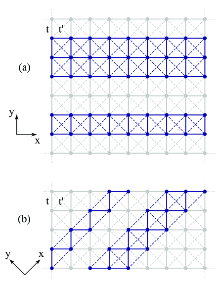
FIG. 1.: 2 and 3-leg ladders on the background lattice. (a) bond-aligned ladders (b) diagonal ladders.

The bond-aligned N-leg ladder is described by the Hamiltonian $H=H_{0}^{\textit{bond}}+H_{U}$

$$H_{0}^{\textit{bond}} = \sum_{i=1}^{N}\sum_{x}\sum_{\sigma=\uparrow,\downarrow}\bigg{\{}$$ (1)

$$- t[c^{{\dagger}}_{i,x,\sigma}c^{\vphantom{{\dagger}}}_{i+1,x,\sigma}+c^{{\dagger}}_{i,x,\sigma}c^{\vphantom{{\dagger}}}_{i,x+1,\sigma}+h.c.]$$ (2)

$$- t^{\prime}[c^{{\dagger}}_{i,x,\sigma}c^{\vphantom{{\dagger}}}_{i+1,x-1,\sigma}+c^{{\dagger}}_{i,x,\sigma}c^{\vphantom{{\dagger}}}_{i+1,x+1,\sigma}+h.c.]\bigg{\}}\;,$$ (3)

$$H_{U} = U\sum_{i=1}^{N}\sum_{x}:n_{i,x,\uparrow}n_{i,x,\downarrow}:\;,$$ (5)

where $c^{\vphantom{{\dagger}}}_{i,x,\sigma}$ annihilates a spin $\sigma$ electron at site $x$ on chain $i$ and $n_{i,x,\sigma}=c^{\dagger}_{i,x,\sigma}c^{\phantom{\dagger}}_{i,x,\sigma}$. For the bond-aligned ladders we take as unit length the distance between nearest neighbors. The on-site Hubbard interaction is assumed weak $U\ll t$.

The diagonal N-leg ladder is described by the Hamiltonian $H=H_{0}^{\textit{diag}}+H_{U}$ where

$$H_{0}^{\textit{diag}} = \sum_{i=1}^{N}\sum_{x}\sum_{\sigma=\uparrow,\downarrow}\bigg{\{}$$ (6)

$$- t[c^{{\dagger}}_{i,x,\sigma}c^{\vphantom{{\dagger}}}_{i+1,x+\frac{1}{2},\sigma}+c^{{\dagger}}_{i,x,\sigma}c^{\vphantom{{\dagger}}}_{i+1,x-\frac{1}{2},\sigma}+h.c.]$$ (7)

$$- t^{\prime}[c^{{\dagger}}_{i,x,\sigma}c^{\vphantom{{\dagger}}}_{i,x+1,\sigma}+c^{{\dagger}}_{i,x,\sigma}c^{\vphantom{{\dagger}}}_{i+2,x,\sigma}+h.c.]\bigg{\}}\;.$$ (8)

For this model we choose the next-nearest-neighbor distance as our unit of length along the $x$ direction. This means that $x$ runs over the integers on odd chains and over the integers shifted by 1/2 on even chains.

We study the above models in the weak-coupling limit using RG techniques. Much of the analysis is identical to the one used in previous studies of Hubbard ladders [20, 21, 22, 23, 24, 25, 26] and consequently we outline here only the basic steps of the procedure, relegating some of the remaining details to the appendix.

Since the interaction term is treated as a perturbation the first step is the diagonalization of the quadratic part of the Hamiltonian via the transformation

$$c_{i,x,\sigma}=\sum_{b=1}^{N}\sum_{k_{x}=-\pi}^{\pi}e^{ik_{x}x}S_{ib}\psi_{b,\sigma}(k_{x})\;,$$ (9)

where the matrix $S$ depends on the specific model. The resulting free band structure is then filled up to the chemical potential (we assume zero temperature throughout the paper) which is determined by the averaged electronic occupation per site $n$. Each band that crosses the chemical potential gives rise to $N_{b}$ symmetric pairs of Fermi points, where more than one pair may exist for a single band, see Fig. 8 for an example. A linearized chiral electronic branch is associated with every Fermi point. In order to have positive definite Fermi velocities we assign left (right) moving fields to Fermi points at which the spectrum is a descending (ascending) function of $k_{x}$. When the expansion of the band field operators in terms of these chiral fields

$$\psi_{b,\sigma}(x)\sim\sum_{j_{b}=1}^{N_{b}}e^{i\eta_{j_{b}}|k_{F_{j_{b}}}|x}\psi_{j_{b},\sigma}^{R}(x)+e^{-i\eta_{j_{b}}|k_{F_{j_{b}}}|x}\psi_{j_{b},\sigma}^{L}(x)\;,$$ (10)

with $\eta={\rm sign}(k_{F})$ at the right moving point, is plugged into the Hubbard term, Eq. (5), a host of interaction terms emerges. Typically only forward- and Cooper-scattering are allowed by momentum and spin conservation [20, 21], but for appropriate values of the parameters other momentum-conserving “special” processes and Umklapp terms appear as well (See Figs. 2,3 and the appendix).

In the first stage of the renormalization process the RG equations for the various coupling constants (as given in the appendix) are integrated numerically until $\l$, the logarithm of the cut-off in units of its initial value, approaches a point $\l^{*}$ where one or more of the couplings grows as $(l-l^{*})^{-\gamma}$ with $\gamma\leq 1$. At this scale the flow has reached the vicinity of a strong-coupling fixed point. The most divergent couplings in this region tend to freeze certain modes and open a gap in their fluctuation spectrum. The pinned modes may be identified via bosonization and the gap scale associated with them may be related to the original bandwidth $E_{F}$ according to

$$\Delta_{1}\approx E_{F}e^{-l^{*}}\;.$$ (11)

To obtain the behavior of the system on scales larger than $l^{*}$ one needs to carry out a second RG stage in which the relevance of the weakly or non-diverging couplings of the first stage is assessed near the new strong-coupling fixed point [22, 26]. This is done by calculating their scaling-dimension $\delta$ while freezing the gapped modes. In case some of these couplings become relevant the flow is directed towards a new fixed point in which additional modes are gapped with a typical scale of

$$\Delta_{2}\approx\Delta_{1}g_{*}^{1/(2-\delta)}\;,$$ (12)

where $g_{*}$ is the dimensionless strength of the residual interactions at the end of the first RG stage [22, 26]. In principle one should repeat the process until a stable fixed point is reached. In our case we find that if new relevant couplings do occur in the second stage, they take the system into the maximally allowed gapped phase.

B Results

Our results for the ladder models are summarized in the phase diagrams as presented in Figs. 2 - 5. To facilitate comparison with the cuprates we concentrate on the case $t^{\prime}<0$[30, 31]. Since the model is defined on a bipartite lattice the spectrum is invariant under $t\rightarrow-t$. Moreover, the particle-hole transformation $c_{x,y,\sigma}\rightarrow c^{\dagger}_{x,y,\sigma}$ maps the original Hamiltonian on itself with $t\rightarrow-t$, $t^{\prime}\rightarrow-t^{\prime}$ and changes the average electronic density according to $n\rightarrow 2-n$. One can therefore obtain the $t^{\prime}>0$ half of the diagrams by reflecting them with respect to the $t^{\prime}=0$ and the $n=1$ lines.

We use the C$m$S$n$ classification scheme[20, 21, 22] wherein a phase is characterized by the number ($m,n$) of its gapless charge and spin modes. In the diagrams we shaded the regions in which the systems end up in the maximally gapped phase (C1S0) allowed by global gauge and translational invariance[22]. In the lightly shaded areas this phase is obtained only at the end of the second RG stage and the nature of the phase at the end of the first stage is shown in parentheses. More information on the character of the massive fields, and the relevant operators which give them their masses, is detailed in the appendix. We find that whenever the C1S0 phase is not reached the systems retain all of their non-interacting gapless modes, as indicated in the clear parts of the diagrams.

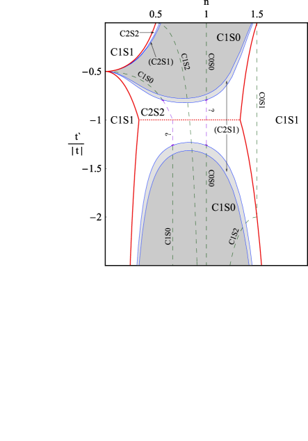
FIG. 2.: The phase diagram of the 2-leg bond-aligned ladder. The system remains gapless in the light regions and exhibits the maximally gapped C1S0 phase in the shaded parts of the diagram. In the darker shaded regions this phase is obtained at the end of the first RG stage while it is reached only at the end of the second stage inside the lightly shaded domains. In the latter case we indicate in parentheses the nature of the phase at the end of the first stage. Umklapp and “special” processes are allowed on the dashed lines. The number of non-interacting Fermi points changes by 2 across the thick solid lines and the Fermi velocity associated with the pair vanishes there. On the dotted line a flat band occurs. Consequently, our results are unreliable in the vicinity of these lines.

For the 2-leg ladders we have also considered the possibility of Umklapp scattering and momentum-conserving “special” processes which exist for particular values of the Fermi wave-vectors. The dashed lines in the diagrams correspond to parameters for which such processes are allowed. In all cases we find that the nature of the resulting phases, as indicated next to the lines, is determined by the end of the first RG stage. Along the sections marked by “?” the relevant terms of the first RG stage tend to pin pairs of canonically conjugated fields. Consequently, we were unable to determine the fate of the system in this eventuality.

Our renormalization procedure relies on the linearization of the non-interacting spectrum around the Fermi points. It therefore fails whenever a pair of Fermi points resides at an extremum of the band structure. This happens along the thick solid lines in the diagrams. Across each of these lines the number of Fermi point pairs changes by 1 (or 2 in the case of a “W” shaped band). For the bond-aligned ladders a flat band arises along the dotted lines in their diagrams while for the 3-leg diagonal ladder such a band occurs for $t^{\prime}=0$ and $2/3<n<4/3$. Our results are unreliable in the vicinity of these lines.

Our most important finding is a correlation between the ladder orientation and the nature of its phase at small values of $t^{\prime}/t$. The bond-aligned ladders exhibit the gapped C1S0 phase over a wide range of electronic filling $0.5\lesssim n\lesssim 1.5$. The diagonal ladders on the other hand remain gapless, except for a small region near $n=1$ in the case of the diagonal 3-legged system.

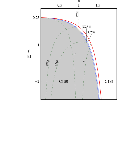
FIG. 3.: The phase diagram of the 2-leg diagonal ladder.

Bond-aligned ladders with $t^{\prime}=0$ have been analyzed in the past using perturbative RG[20, 21, 22, 23, 24, 25, 26] and in most cases were found to be in the C1S0 phase[32]. This conclusion was further supported by density matrix renormalization group (DMRG) calculations at strong-coupling [14, 15, 16, 17, 18]. Our results demonstrate the robustness of this phase in the presence of not too large next-nearest-neighbor hopping. Our results also agree with the gapless behavior found in a previous DMRG study of the diagonal 2-leg ladder[19] and add information about this system at commensurate fillings. We are unaware of past treatments of the 3-leg diagonal ladder, especially in the strong interaction regime. It is therefore unclear whether the gapless phase found by us in this model survives beyond the limit of weak-coupling. It is, however, interesting to note that at half filling and for $t^{\prime}=0$ and $U\rightarrow\infty$, the diagonal 3-leg ladder is equivalent to an alternating spin-1 and spin-1/2 chain, which is known to be gapless[33].

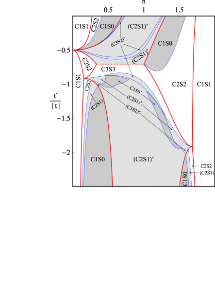
FIG. 4.: The phase diagram of the 3-leg bond-aligned ladder. To distinguish between gapped phases which originate from a C2S2 phase, and those coming from a C3S3 phase, we mark the latter by an asterisk.

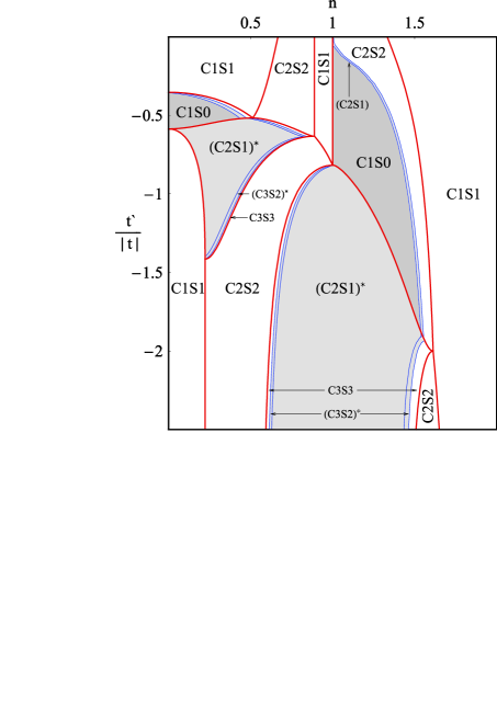
FIG. 5.: The phase diagram of the 3-leg diagonal ladder.

One may estimate the gap scale in the gapped phases from Eqs. (11,12). Typically we find that the gap changes smoothly across boundaries between adjacent extended C1S0 phases, regardless of the RG stage at which they become fully gapped. One exception is the 3-leg bond-aligned ladder at small $t^{\prime}/t$ where the gap increases considerably in the region around $n=1$ due to a much smaller $l^{*}$ (which, in passing, we note scales as $t/U$). The gap is very small in the sliver phases.

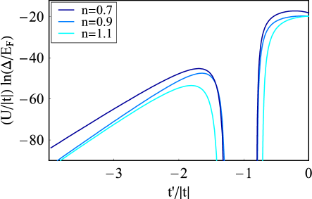
FIG. 6.: Gap scale in the 2-leg bond-aligned ladder.

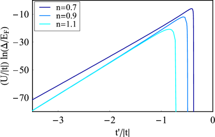
FIG. 7.: Gap scale in the 2-leg diagonal ladder.

The dependence of $\Delta$ on $t^{\prime}$ for the 2-leg ladders is presented in Figs. 6,7. Increasing the magnitude of the next-nearest-neighbor hopping results in a decrease of the gap in the bond-aligned system. On the contrary, the diagonal ladder, which is gapless for $t^{\prime}=0$, develops a gap above a critical density-dependent value of $t^{\prime}$. Further increase of the hopping amplitude causes the gap to grow, reach a maximum and then decrease. We observe a similar behavior also in the 3-leg ladders.

III Stripes as defects in an antiferromagnetic background

A Model

Since the cuprate high-temperature superconductors are born out of parent antiferromagnets one expects to find slow fluctuations of a collective field representing the local staggered magnetization. Stripes may be thought of as defects in this field along which holes tend to segregate. In the previous section we have assumed that the confinement of the holes to the stripes is extremely strong such that their coupling to the antiferromagnetic environment may be neglected. Here we would like to relax this constraint. To do so we consider a model of non-interacting electrons on the square lattice interacting with a static staggered field

$$H_{0}^{\textit{defect}} = \sum_{x,y}\sum_{\sigma=\uparrow,\downarrow}\bigg{\{}$$ (13)

$$- t[c^{{\dagger}}_{x,y,\sigma}c^{\vphantom{{\dagger}}}_{x+1,y,\sigma}+c^{{\dagger}}_{x,y,\sigma}c^{\vphantom{{\dagger}}}_{x,y+1,\sigma}+h.c.]$$ (14)

$$- t^{\prime}[c^{{\dagger}}_{x,y,\sigma}c^{\vphantom{{\dagger}}}_{x-1,y+1,\sigma}+c^{{\dagger}}_{x,y,\sigma}c^{\vphantom{{\dagger}}}_{x+1,y+1,\sigma}+h.c.]$$ (15)

$$+ \sigma(-1)^{x+y}m(x,y)c^{{\dagger}}_{x,y,\sigma}c^{\vphantom{{\dagger}}}_{x,y,\sigma}\bigg{\}}\;,$$ (16)

where $c^{\vphantom{{\dagger}}}_{x,y,\sigma}$ annihilates a spin $\sigma$ electron at site $(x,y)$ on the lattice (as defined in the coordinate system of Fig. 1a.) The field configuration is taken to represent defects with the same geometries as the ladders studied in Section II

$$m(x,y)=\begin{cases}m&\text{left of ladder}\\ 0&\text{on the ladder}\\ \pm m&\text{right of ladder}\;.\\ \end{cases}$$ (17)

We consider both in-phase ($+m$) and anti-phase ($-m$) domain walls.

In the absence of a defect, i.e. $m(x,y)=m$, the spectrum exhibits two bands of extended Bloch states whose energies $E=-4t^{\prime}\cos(k_{x})\cos(k_{y})\pm\sqrt{4t^{2}[\cos(k_{x})+\cos(k_{y})]^{2}+m^{2}}$ are separated by an energy gap of order $m$ for large enough magnetization. Introducing a domain wall into the periodic background leads to the appearance of mid-gap states, see Fig. 8. These states are localized in the transverse direction to the wall[29] over a distance which typically scales as $m^{-1}$. We therefore expect their energies to approach, in the limit $m\rightarrow\infty$, the non-interacting energies of the corresponding ladder.

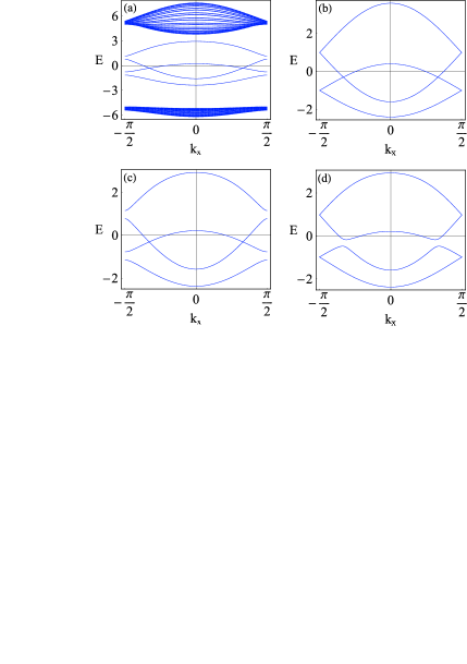
FIG. 8.: The band structure of the 2-leg bond-aligned defect for $t^{\prime}/t=-0.3$. (a) The full spectrum including the bands of extended states for the case of an anti-phase defect with $m/t=5$, (b) the localized bands for infinite $m$, (c) the localized bands of the anti-phase defect with $m/t=5$, (d) the localized bands of the in-phase defect with $m/t=5$.

In the following we assume that $m$ is large enough, such that varying the density of the system away from half filling is achieved by doping electrons or holes solely into the mid-gap bands. Consequently, we consider a reduced model whose non-interacting spectrum is composed of these localized mid-gap bands only. This band structure expresses, albeit on a coarse mean-field level, the effects of interactions between the electrons on the defect and the electrons comprising the antiferromagnetic background. In the cuprates these interactions are expected to be of similar magnitude to the interactions between the electrons moving along the stripes. However, in our perturbative treatment the latter are assumed much weaker. While unjustified when modeling real stripes this assumption enables us to treat the interactions on the defect in a controlled manner and gain some insight into the effects of the coupling between stripes and their antiferromagnetic environment.

To make contact with the ladder models of the previous section we relate the electronic operators on the defect sites to the creation operators of the localized states. The result is analogous to Eq. (9) with two differences. First, the exact expansion of the site operators generally includes components along extended states. Such components are projected out and the remaining sum is properly normalized. As long as the mid-gap states are well localized on the defect the projected expansion remains a faithful representation of the site operators on the stripe. Secondly, for an $N$-leg bond-aligned defect the staggered field induces a doubling of the unit-cell and of the number of localized bands. Accordingly, in Eq. (9), $x$ becomes the unit-cell coordinate and $i$ stands for the leg number together with the site index within the unit-cell. The sum over the band index then runs from 1 to $2N$ and the sum over the momentum along the defect extends from $-\pi/2$ to $\pi/2$. This effect is absent in the case of diagonal stripes. On the other hand, and in contrast to the bond-aligned systems, the spin degeneracy of the bands is lifted whenever the spin texture is symmetric on opposite sides of a diagonal defect [this happens in anti-(in-) phase defects with even(odd) $N$].

From this point onward the analysis of the interactions between electrons on the defect, as given by the Hubbard term Eq. (5), follows the same course described for the ladder models. However, owing to the absence of spin SU(2) symmetry in this case, we are compelled to consider, separately, scattering processes in different spin channels.[25] The resulting RG equations will be given elsewhere.

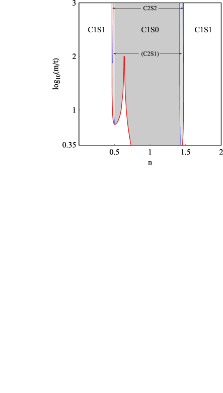
FIG. 9.: The dependence of the phase diagram of an anti-phase 2-leg bond-aligned defect on the magnetization $m$. The results are for the case $t^{\prime}/t=-0.1$.

B Results

In Fig. 9 we present the phase diagram of the anti-phase bond-aligned 2-leg defect as a function of $m$ and $n$ for a fixed small value of $t^{\prime}$. We already referred to the fact that identifying the mid-gap sector of the spectrum with the electronic states of a stripe makes sense as long as these states are well localized on the defect. Since the localization length becomes larger with decreasing magnetization or increasing next-nearest-neighbor hopping it imposes a limit on the minimal $m$ and maximal $t^{\prime}/t$ which may be studied using this model. This constraint sets the lower bound of the magnetization axis in the figure.

As can be seen lowering the modulation depth of the antiferromagnetic environment leads eventually to a reduction in the extent of the gapped phase. The corresponding diagram for the analogous in-phase system, on the other hand, shows no significant changes in the phase boundaries down to the lowest value of $m$. A similar result is obtained for the 3-leg bond-aligned defects, with the exception that it is the in-phase system whose gapped phase is depleted at small $m$ while the diagram of the anti-phase defect remains largely unaffected. We are therefore led to the conclusion that a larger sensitivity to changes in $m$ exists when spins across the defect are aligned.

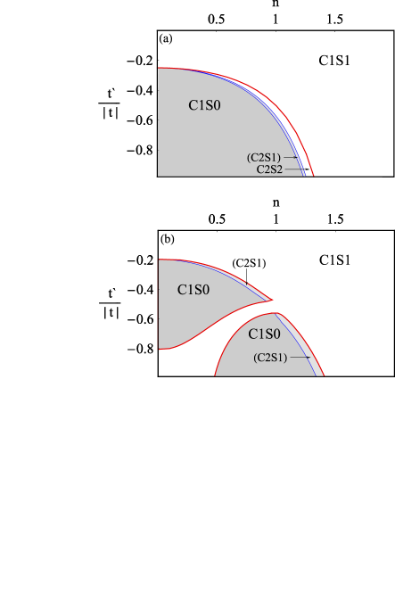
FIG. 10.: A comparison between the phase diagrams of (a) the 2-leg diagonal ladder and (b) the in-phase 2-leg diagonal defect with $m=3.5$.

The changes in the phase diagrams are initiated by deformations in the non-interacting band-structure as $m$ is reduced. For infinite $m$ the mid-gap spectrum of the defect is identical to that of the corresponding ladder. For finite magnetization some of the degenerate points in the spectrum of the ladder separate by mini-gaps. When the background spin texture is symmetrical with respect to the defect the degeneracy at $k_{x}=\pi/2$ is lifted. When it is asymmetrical the bands separate at $k_{x}$ values away from the edge of the Brillouin zone, see Fig. 8. When a separation occurs, the result may be the removal of two Fermi points from the system (an example appears in Fig. 8c around $E=-1$). Such an event typically leads to a transition from a gapped to a gapless phase. In the symmetrical case, this scenario is more frequent, a fact which explains why it is more sensitive to variations in $m$. Opposite occurrences where a band deforms from a “U” to a “W” shape, with the result of the appearance of an additional pair of Fermi points, are also possible but are less common. These changes lead to fragmentation of the phase diagrams of the defects. Usually gapped phases are being penetrated by extensions of gapless phases, but we also encounter pockets or slivers of strong (first RG stage) C1S0 phase inside regions which are gapless or weakly gapped in the ladder system.

We already mentioned that the spin degeneracy of the spectrum is lifted in the anti-phase 2-leg and the in-phase 3-leg diagonal defects. In these cases the RG analysis indicates that the coupling constants do not flow and the systems remain in their gapless non-interacting phases. The spectra of the related systems with anti-symmetric spin configurations across the defects are still spin-degenerate and contain similar openings of mini-gaps as the bond-aligned defects. Consequently, their phase diagrams exhibit a more fragmented behavior, as demonstrated by Fig. 10.

We find that lowering the magnitude of the staggered field diminishes the extent of the C2S2 phase throughout the phase diagrams. This effect is especially significant in the case of the 3-leg anti-phase diagonal defect where it leads to a reduction in the extent of the gapless phase in small t’/t, narrowing it down to a region centered around half filling.

IV Discussion

The results presented in this paper were derived for weak interaction strength $U$ where all gap scales are exponentially small. It is unclear to what extent they represent the properties of ladders at strong coupling. However, based on past experience coming from numerical studies [14, 15, 16, 17, 18, 19], it seems that many of the qualitative features of doped Hubbard ladders, such as the nature of their low-energy phases, are robust against changes in the interaction strength. In the following we assume that such continuity holds also for our results and, keeping in mind the other limitations of modeling hole-rich stripes as doped ladders, comment on their possible relevance to the physics of the cuprate high-temperature superconductors.

By now a large body of experimental data points to the fact that inhomogeneous electronic structures are prevalent in the cuprates [1]. There is no consensus, however, on the role played by such inhomogeneities in the formation of high-temperature superconductivity and the other unique features of these compounds. One view, identifies the scattering of quasiparticles from the critical charge fluctuations associated with a stripe quantum critical point, as responsible for the anomalous electronic properties, such as the pseudogap in the underdoped regime [34, 35]. Another view, stipulates that the spin-gap, which develops on stripes, is the source of the pseudogap [24]. The opening of this gap leads to intra-stripe power-law superconducting correlations, which turn eventually, via inter-stripe Josephson pair-tunneling, into global long-range superconducting order.

For stripes to play an essential role in the physics of the cuprates they must exist, either as static order or as fluctuating correlations, above the pseudogap crossover and the superconducting transition temperatures. Moreover, if the second point of view, just mentioned, is correct, these stripes must support a gap in order for superconductivity to be achieved.

As indicated in the introduction La_2-xSr_xCuO₄ is a system where the existence of stripes is very well established over a wide range of hole-dopings and temperatures. As such it fulfills the first requirement. Our finding that under generic conditions weakly interacting diagonal ladders are gapless while bond-aligned ladders possess a spin-gap, offers some support to the hypothesis that a similar difference between the low-energy properties of bond-aligned and diagonal stripes is behind the coincidence of the insulator-superconductor transition and the rotation of the stripes direction in this compound[36]. It also supports the identification of bond-aligned stripes as the origin of the gapped ARPES spectrum around $(\pi,0)$ (and symmetry related points) in $\vec{k}$-space, and the association of the gapless Fermi surface at $(\pi/2,\pi/2)$ with diagonal stripes.

One may raise, however, difficulties associated with this picture. The first concerns signs of gapped components in the spin-glass phase of La_2-xSr_xCuO₄ with $x\leq 0.05$. ARPES measurements have found a distinctive “knee” in the energy distribution curves at $(\pi,0)$ in $x=0.05$ samples[37, 38, 39]. This feature appears at a binding energy of about 0.1 eV and becomes more prominent and less gapped with increased doping levels. It is consistent, within experimental uncertainties involving the doping, with the bond-aligned incommensurate signal observed in elastic neutron-scattering experiments[5]. This signal coexists with incommensurate diagonal peaks for $0.056\leq x\leq 0.07$ and grows stronger with $x$. There is, however, some evidence coming from ARPES[37, 38, 39] that a similar but faint gapped band exists also in $x=0.03$ samples for which no corresponding neutron-scattering signal has been reported.

A more serious objection, perhaps, may be raised in connection to the existence of a gapless diagonal component well inside the superconducting regime. A peak in the ARPES spectrum near $(\pi/2,\pi/2)$ and at the Fermi energy exists in all samples with $0.03\leq x\leq 0.15$ (and beyond)[39, 38]. Its spectral weight intensifies upon entering the superconducting region and continues to grow at least until optimal doping[39]. Although the above mentioned coexistence of bond-aligned and diagonal incommensurate neutron-scattering peaks might explain this behavior near the insulator-superconductor transition, it does not offer an explanation at higher doping levels. One possible solution to the problem is that diagonal stripes continue to exist deep in the superconducting phase, but only as fluctuating correlations. Such slowly fluctuating bond-aligned incommensurate correlations have been observed in inelastic neutron-scattering measurements of La_2-xSr_xCuO₄ with $0.12\leq x\leq 0.27$[2, 40]. Their detection along the diagonal directions would tie La_2-xSr_xCuO₄ with another member of the cuprate family, YBa₂Cu₃O_7-δ , in which an anisotropic incommensurate ring was recently found by inelastic neutron-scattering experiments on underdoped and nearly optimally doped samples[41].

A The RG Procedure for the ladder models

1 Cooper- and forward-scattering

As mentioned previously, spin and momentum conservation generically allows only for Cooper- and forward-scattering[21]. These processes are conveniently described using the charge and spin currents

$$J^{R}_{ij} = \sum_{\alpha}:\psi^{R{\dagger}}_{i\alpha}(x)\psi^{R}_{j\alpha}(x):\;,$$ (A1)

$$\mathchoice{{\hbox{\boldmath$\displaystyle J$}}}{{\hbox{\boldmath$\textstyle J$}}}{{\hbox{\boldmath$\scriptstyle J$}}}{{\hbox{\boldmath$\scriptscriptstyle J$}}}^{R}_{ij} = \frac{1}{2}\sum_{\alpha,\beta}:\psi^{R{\dagger}}_{i\alpha}(x)\mathchoice{{\hbox{\boldmath$\displaystyle\sigma$}}}{{\hbox{\boldmath$\textstyle\sigma$}}}{{\hbox{\boldmath$\scriptstyle\sigma$}}}{{\hbox{\boldmath$\scriptscriptstyle\sigma$}}}_{\alpha\beta}\psi^{R}_{j\beta}(x):\;,$$ (A2)

where $\textstyle\sigma$ denotes the Pauli matrices. The same definitions apply for the left components. The allowed terms are

$$H_{int} = \int\!dx\sum_{i,j=1}^{N}\pi(v_{i}+v_{j})\bigg{\{}c^{\rho}_{ij}J^{R}_{ij}J^{L}_{ij}-c^{\sigma}_{ij}\mathchoice{{\hbox{\boldmath$\displaystyle J$}}}{{\hbox{\boldmath$\textstyle J$}}}{{\hbox{\boldmath$\scriptstyle J$}}}{{\hbox{\boldmath$\scriptscriptstyle J$}}}^{R}_{ij}\cdot\mathchoice{{\hbox{\boldmath$\displaystyle J$}}}{{\hbox{\boldmath$\textstyle J$}}}{{\hbox{\boldmath$\scriptstyle J$}}}{{\hbox{\boldmath$\scriptscriptstyle J$}}}^{L}_{ij}$$ (A3)

$$+ f^{\rho}_{ij}J^{R}_{ii}J^{L}_{jj}-f^{\sigma}_{ij}\mathchoice{{\hbox{\boldmath$\displaystyle J$}}}{{\hbox{\boldmath$\textstyle J$}}}{{\hbox{\boldmath$\scriptstyle J$}}}{{\hbox{\boldmath$\scriptscriptstyle J$}}}^{R}_{ii}\cdot\mathchoice{{\hbox{\boldmath$\displaystyle J$}}}{{\hbox{\boldmath$\textstyle J$}}}{{\hbox{\boldmath$\scriptstyle J$}}}{{\hbox{\boldmath$\scriptscriptstyle J$}}}^{L}_{jj}\bigg{\}}\;,$$ (A4)

where $v_{i}$ is the Fermi velocity at $k_{F_{i}}$. $f_{ij}$ and $c_{ij}$ are the forward- and Cooper-scattering amplitudes respectively. As $f_{ii}$ and $c_{ii}$ describe the same process we take $f_{ii}=0$.

The RG equations for these couplings and their bare values in terms of $U$ and the transformation matrix $S$ introduced in Eq. (9) have been derived by Lin, Balents and Fisher in Ref. A 2. The most diverging couplings, as found by numerical integration of the RG equations, determine the nature of the phase on the scale at which the divergence occur. Subsequent scaling-dimension analysis determines the ultimate character of the system on even longer scales. The precise point at which a particular operator is declared most relevant is somewhat arbitrary. This uncertainty might affect the extent of the phases identified. Notwithstanding, we have verified the robustness of our results with respect to small variations in this criterion. Note that we chose not to display in the phase diagrams, Figs. 2-5, some of the phases whose ranges were found to be very small.

When none of the couplings diverge the result is a gapless phase. The scaling-dimension analysis indicates that all the couplings are marginal, thus ensuring the stability of the resulting C$n$S$n$ phase (where $n$ denotes the number of pairs of Fermi points).

A C$n$S$n$-1 phase is obtained at the end of the first renormalization stage when a single $c^{\sigma}_{aa}$ coupling diverges. The bosonized relevant interaction is proportional to $c^{\sigma}_{aa}\cos(\sqrt{8\pi}\phi_{a}^{\sigma})$ and results in a single gapped spin mode. A scaling-dimension analysis, after freezing $\phi_{a}^{\sigma}$, indicates that the interactions $c^{\sigma}_{aj}\cos[\sqrt{2\pi}(\theta_{a}^{\rho}-\theta_{j}^{\rho})]\cos(\sqrt{2\pi}\phi_{j}^{\sigma})$ become relevant. They lead to a new C1S0 fixed point.

The maximally allowed gapped phase, C1S0, is reached at the end of the first RG stage when all couplings except $f^{\sigma}_{ij}$ diverge. When this happens $c_{ij}^{\sigma}(l^{*})\approx 4c_{ij}^{\rho}(l^{*})$ and the relevant interactions take the form

$$\propto\sum_{i,j} (v_{i}+v_{j})$$ (A6)

$$\times c^{\sigma}_{ij}\cos[\sqrt{2\pi}(\theta_{i}^{\rho}-\theta_{j}^{\rho})]\cos(\sqrt{2\pi}\phi_{i}^{\sigma})\cos(\sqrt{2\pi}\phi_{j}^{\sigma})\;.$$

The terms with $i=j$ pin all the spin modes. The terms with $i\neq j$ imply $n-1$ gapped charge modes. The outcome is correspondingly a C1S0 phase.

In the region where three pairs of Fermi points exist we encounter a situation in which all the couplings associated with two Fermi point pairs ($a,b$) diverge at the end of the first RG stage, except for $f^{\sigma}_{ab}$. The relevant interactions are then similar to those of Eq. (LABEL:relevant), where $i$ and $j$ take the values $a,b$. The $i=j$ terms lead to two gapped spin modes. The $i\neq j$ terms result in one gapped charge mode which is associated with $\theta_{ab}^{\rho-}=(\theta_{a}^{\rho}-\theta_{b}^{\rho})/\sqrt{2}$.

The stability of the resulting C2S1 phase is determined by the value of $K_{ab}^{\rho+}$, the Luttinger exponent of $\theta_{ab}^{\rho+}=(\theta_{a}^{\rho}+\theta_{b}^{\rho})/\sqrt{2}$. When $1/K_{ab}^{\rho+}<4$ the interactions associated with $c_{ac}^{\sigma}$ and $c_{bc}^{\sigma}$ become relevant and the system ends up once again in the C1S0 phase. The value of this Luttinger exponent[20]

$$(K_{ab}^{\rho+})^{-2}=$$ (A8)

$$\frac{4\nu[4\nu^{2}-4\nu(1+\nu)^{2}f_{ab}^{\rho*}+(\nu^{2}-1)^{2}(f_{ab}^{\rho*})^{2}]}{(1+\nu)^{2}[2\nu+(\nu-1)^{2}f_{ab}^{\rho*}][2\nu-(1+6\nu+\nu^{2})f_{ab}^{\rho*}]}\;,$$ (A9)

where $\nu=v_{a}/v_{b}$, depends on $f_{ab}^{\rho*}$, the forward-scattering amplitude between the spin-gapped bands at the end of the first RG stage, as shown in Fig. 11. One can see that $1/K_{ab}^{\rho+}<1$, except for a narrow region whose location varies from 1/4 to 0 as $\nu$ deviates from 1. Therefore, although the exact value of $f_{ab}^{\rho*}$ is not known precisely, we may conclude that the system eventually flows to a C1S0 phase.

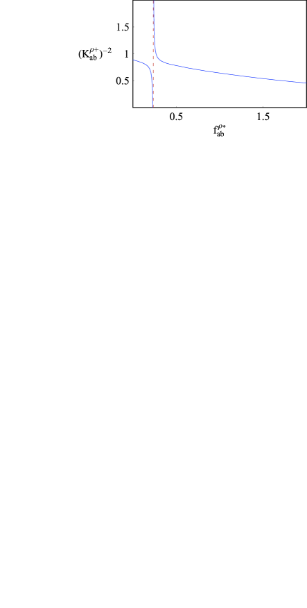
FIG. 11.: Typical behavior of the Luttinger exponent of $\theta_{ab}^{\rho+}$ when $\theta_{ab}^{\rho-}$ is frozen.

2 Umklapp and “special” processes

Umklapp scattering and “special” processes which preserve momentum but exist only for specific values of the Fermi wave-vectors[42] are allowed on special lines in parameter space, as shown, for example, in the phase diagrams of the 2-leg ladders. In the following we describe all the Umklapp and “special” terms in the presence of two pairs of Fermi points. For this purpose we define

$$K_{i\alpha j\beta}^{R}=:\psi^{R}_{i\alpha}(x)\psi^{R}_{j\beta}(x):\;.$$ (A10)

An intra-band Umklapp term exists in the case where one of the Fermi points pairs resides at $k_{F_{i}}=\pi/2$,

$$H_{Umklapp}^{(1)}=\int\!dx\sum_{\alpha,\beta}2\pi v_{i}u_{ii}\left[K_{i\alpha i\beta}^{R\dagger}K_{i\alpha i\beta}^{L}+h.c.\right]\,.$$ (A11)

The RG equation for the single-band Cooper-scattering $c_{ii}^{\rho}$ is altered by this Umklapp process. Denoting the addition to the RG equation as $\delta c_{ii}$ we find

$$\delta\dot{c}^{\rho}_{ii}=4(u_{ii})^{2}\;,$$ (A12)

where the dot indicates a derivative with respect to the length-scale $l$. An additional RG equation for the Umklapp coupling itself is needed,

$$\dot{u}_{ii}=4c^{\rho}_{ii}u_{ii}\;,$$ (A13)

with the initial value $u_{ii}=U/8\pi v_{i}$ for the systems that we have considered.

When the sum of $k_{F_{i}}$ and $k_{F_{j}}$ at the right moving Fermi points equals $\pi$, three inter-pair Umklapp interactions emerge.

$$H_{Umklapp}^{(2)} = \int\!dx\sum_{\alpha,\beta}\pi(v_{i}+v_{j})$$ (A14)

$$\times \bigg{\{}u_{ij}^{a}\left[K_{i\alpha i\beta}^{R\dagger}K_{j\alpha j\beta}^{L}+K_{j\alpha j\beta}^{R\dagger}K_{i\alpha i\beta}^{L}+h.c\right]$$ (A15)

$$+ u_{ij}^{b}\left[K_{i\alpha j\beta}^{R\dagger}K_{i\alpha j\beta}^{L}+h.c.\right]$$ (A16)

$$- u_{ij}^{c}\left[K_{i\alpha j\beta}^{R\dagger}K_{j\alpha i\beta}^{L}+h.c.\right]\>+\>i\leftrightarrow j\bigg{\}}\;.$$ (A17)

The same scattering processes also exist, as momentum-conserving “special terms”, when the two wave-vectors equal each other. These interactions induce additional terms in the Cooper- and forward-scattering RG equations

$$\delta\dot{c}^{\rho}_{ii} = 4\alpha_{ij}(u_{ij}^{b})^{2}+4\alpha_{ij}(u_{ij}^{c})^{2}+4\alpha_{ij}u_{ij}^{b}u_{ij}^{c}\;,$$ (A18)

$$\delta\dot{c}^{\sigma}_{ii} = -16\alpha_{ij}(u_{ij}^{b})^{2}-16\alpha_{ij}u_{ij}^{b}u_{ij}^{c}\;,$$ (A19)

$$\delta\dot{f}^{\rho}_{ij} = 16(u_{ij}^{a})^{2}+4(u_{ij}^{b})^{2}+4(u_{ij}^{c})^{2}+4u_{ij}^{b}u_{ij}^{c}\;,$$ (A20)

$$\delta\dot{f}^{\sigma}_{ij} = -16(u_{ij}^{c})^{2}-16u_{ij}^{b}u_{ij}^{c}\;,$$ (A21)

$$\delta\dot{c}^{\rho}_{ij} = 8u_{ij}^{a}(u_{ij}^{b}-u_{ij}^{c})\;,$$ (A22)

$$\delta\dot{c}^{\sigma}_{ij} = 32u_{ij}^{a}(u_{ij}^{b}+u_{ij}^{c})\;,$$ (A23)

where $\alpha_{ij}=(v_{i}+v_{j})^{2}/4v_{i}v_{j}$. The RG equations for the new couplings are

$$\dot{u}_{ij}^{a} = 4f_{ij}^{\rho}u_{ij}^{a}+c_{ij}^{\rho}(u_{ij}^{b}-u_{ij}^{c})+\frac{3}{4}c_{ij}^{\sigma}(u_{ij}^{b}+u_{ij}^{c})\;,$$ (A24)

$$\dot{u}_{ij}^{b} = u_{ij}^{a}(4c_{ij}^{\rho}+c_{ij}^{\sigma})+u_{ij}^{b}(c_{ii}^{\rho}+c_{jj}^{\rho})-\frac{3}{4}u_{ij}^{b}(c_{ii}^{\sigma}+c_{jj}^{\sigma})$$ (A25)

$$+ u_{ij}^{b}(2f_{ij}^{\rho}+\frac{1}{2}f_{ij}^{\sigma})-\frac{1}{2}u_{ij}^{c}(c_{ii}^{\sigma}+c_{jj}^{\sigma})\;,$$ (A26)

$$\dot{u}_{ij}^{c} = u_{ij}^{a}(-4c_{ij}^{\rho}+c_{ij}^{\sigma})-u_{ij}^{b}f_{ij}^{\sigma}+u_{ij}^{c}(c_{ii}^{\rho}+c_{jj}^{\rho})$$ (A27)

$$+ \frac{1}{4}u_{ij}^{c}(c_{ii}^{\sigma}+c_{jj}^{\sigma})+2u_{ij}^{c}f_{ij}^{\rho}-\frac{3}{2}u_{ij}^{c}f_{ij}^{\sigma}\;,$$ (A28)

with the initial values $u_{ij}^{a}=U/8\pi(v_{i}+v_{j})$, $u_{ij}^{b}=U/4\pi(v_{i}+v_{j})$, $u_{ij}^{c}=-U/4\pi(v_{i}+v_{j})$.

More inter-pair Umklapp processes exist when the difference between $k_{F_{i}}$ and $k_{F_{j}}$ at the right moving Fermi points equals $\pi$,

$$H_{Umklapp}^{(3)}=\int\!dx\pi(v_{i}+v_{j})\Big{[}u^{\rho}_{ij}J^{R}_{ij}J^{L}_{ji}+u^{\sigma}_{ij}\mathchoice{{\hbox{\boldmath$\displaystyle J$}}}{{\hbox{\boldmath$\textstyle J$}}}{{\hbox{\boldmath$\scriptstyle J$}}}{{\hbox{\boldmath$\scriptscriptstyle J$}}}^{R}_{ij}\cdot\mathchoice{{\hbox{\boldmath$\displaystyle J$}}}{{\hbox{\boldmath$\textstyle J$}}}{{\hbox{\boldmath$\scriptstyle J$}}}{{\hbox{\boldmath$\scriptscriptstyle J$}}}^{L}_{ji}\>+\>i\!\leftrightarrow\!j\Big{]}.$$ (A29)

The additions to the Cooper- and forward-scattering RG equations are in this case

$$\delta\dot{c}^{\rho}_{ii} = \alpha_{ij}(u_{ij}^{\rho})^{2}+\frac{3}{16}\alpha_{ij}(u_{ij}^{\sigma})^{2}\;,$$ (A30)

$$\delta\dot{c}^{\sigma}_{ii} = -2\alpha_{ij}u_{ij}^{\rho}u_{ij}^{\sigma}-\frac{1}{2}\alpha_{ij}(u_{ij}^{\sigma})^{2}\;,$$ (A31)

$$\delta\dot{f}^{\rho}_{ij} = -(u_{ij}^{\rho})^{2}-\frac{3}{16}(u_{ij}^{\sigma})^{2}\;,$$ (A32)

$$\delta\dot{f}^{\sigma}_{ij} = 2u_{ij}^{\rho}u_{ij}^{\sigma}-\frac{1}{2}(u_{ij}^{\sigma})^{2}\;,$$ (A33)

and the RG equations for these Umklapp couplings are:

$$\dot{u}_{ij}^{\rho} = u_{ij}^{\rho}(c_{ii}^{\rho}+c_{jj}^{\rho}-2f_{ij}^{\rho})-\frac{3}{16}u_{ij}^{\sigma}(c_{ii}^{\sigma}+c_{jj}^{\sigma}-2f_{ij}^{\sigma})\;,$$ (A34)

$$\dot{u}_{ij}^{\sigma} = -u_{ij}^{\rho}(c_{ii}^{\sigma}+c_{jj}^{\sigma}-2f_{ij}^{\sigma})+u_{ij}^{\sigma}(c_{ii}^{\rho}+c_{jj}^{\rho}-2f_{ij}^{\rho})$$ (A35)

$$- \frac{1}{2}u_{ij}^{\sigma}(c_{ii}^{\sigma}+c_{jj}^{\sigma}+2f_{ij}^{\sigma})\;,$$ (A36)

with the initial values $u_{ij}^{\rho}=U/4\pi(v_{i}+v_{j})$, $u_{ij}^{\sigma}=-U/\pi(v_{i}+v_{j})$.

In the diagonal 2-leg ladder, interactions that involve an odd number of operators per band are allowed on specific lines. For example, when the sum of $k_{F_{i}}$ and $3k_{F_{j}}$ at the right moving Fermi points equals zero or equals $2\pi$, we find:

$$H_{Umklapp}^{(4)} = \int\!dx\sum_{\alpha,\beta}\pi(v_{i}+v_{j})u^{d}_{ij}\Big{[}K_{i\alpha j\beta}^{R\dagger}K_{j\alpha j\beta}^{L}$$ (A37)

$$+ K_{i\alpha j\beta}^{L\dagger}K_{j\alpha j\beta}^{R}+h.c\Big{]}\;.$$ (A38)

This coupling induces the following modifications to the RG flow equations

$$\delta\dot{c}^{\rho}_{jj} = 2\beta_{ij}(u_{ij}^{d})^{2}\;,$$ (A39)

$$\delta\dot{c}^{\rho}_{ij} = \beta_{ij}(u_{ij}^{d})^{2}\;,$$ (A40)

$$\delta\dot{f}^{\rho}_{ij} = \beta_{ij}(u_{ij}^{d})^{2}\;,$$ (A41)

where $\beta_{ij}=(v_{i}+v_{j})/2v_{j}$. The additional RG equation is

$$\dot{u}_{ij}^{d}=2u_{ij}^{d}\left(c^{\rho}_{jj}+c^{\rho}_{ij}+f^{\rho}_{ij}\right)\;,$$ (A42)

with the initial value $u_{ij}^{d}=U/2\pi(v_{i}+v_{j})$.

In the case that the difference between $3k_{F_{i}}$ and $k_{F_{j}}$ at the right moving Fermi points equals $2\pi$, the Hamiltonian is:

$$H_{Umklapp}^{(5)}\! = \!\int\!dx\!\sum_{\alpha,\beta}\pi(v_{i}+v_{j})u^{e}_{ij}\Big{[}K_{i\alpha i\beta}^{R\dagger}:\!\psi^{L}_{i\alpha}(x)\psi^{R}_{j\beta}(x)\!:$$ (A43)

$$+ K_{i\alpha i\beta}^{L\dagger}:\!\psi^{R}_{i\alpha}(x)\psi^{L}_{j\beta}(x)\!:+h.c\Big{]}\;.$$ (A44)

The additions to the Cooper- and forward-scattering RG equations in this case are

$$\delta\dot{c}^{\rho}_{ij} = -\frac{1}{2}\beta_{ji}(u_{ij}^{e})^{2}\;,$$ (A45)

$$\delta\dot{c}^{\sigma}_{ij} = 2\beta_{ji}(u_{ij}^{e})^{2}\;.$$ (A46)

The RG equation for the new coupling is

$$\dot{u}_{ij}^{e}=u_{ij}^{e}\left(2c^{\rho}_{ii}-f^{\rho}_{ij}-f^{\sigma}_{ij}\right)\;,$$ (A47)

with the initial value $u_{ij}^{e}=U/2\pi(v_{i}+v_{j})$.

REFERENCES

- [1] For recent reviews of some of the experimental evidence for the existence of meso-structure in the cuprates and its possible relation to the mechanism of high temperature superconductivity see E. W. Carlson, V. J. Emery, S. A. Kivelson, and D. Orgad in “The Physics of Conventional and Unconventional Superconductors”, Vol 2, edited by K. H. Bennemann and J. B. Ketterson (Springer-Verlag 2004), and S. A. Kivelson, I. P. Bindloss, E. Fradkin, V. Oganesyan, J. M. Tranquada, A. Kapitulnik, and C. Howald, Rev. Mod. Phys. 75, 1201 (2003).
- [2] S. Wakimoto, H. Zhang, K. Yamada, I. Swainson, H. Kim, and R. J. Birgeneau, Phys. Rev. Lett. 92, 217004 (2004).
- [3] S. Wakimoto, R. J. Birgeneau, M. A. Kastner, Y. S. Lee, R. Erwin, P. M. Ghering, S. H. Lee, M. Fujita, K. Yamada, Y. Endoh, K. Hirota, and G. Shirane, Phys. Rev. B 61, 3699 (2000).
- [4] M. Matsuda, M. Fujita, K. Yamada, R. J. Birgeneau, M. A. Kastner, H. Hiraka, Y. Endoh, S. Wakimoto, and G. Shirane, Phys. Rev. B 62, 9148 (2000).
- [5] M. Fujita, K. Yamada, H. Hiraka, P. M. Gehring, S. H. Lee, S. Wakimoto, and G. Shirane, Phys. Rev. B 65, 064505 (2002).
- [6] K. Yamada, C. H. Lee, K. Kurahashi, J. Wada, S. Wakimoto, S. Ueki, H. Kimura, Y. Endoh, S. Hosoya, G. Shirane, R. J. Birgeneau, M. Greven, M. A. Kastner, and Y. J. Kim, Phys. Rev. B 57, 6165 (1998).
- [7] T. Suzuki, T. Goto, K. Chiba, T. Shinoda, T. Fukase, H. Kimura, K. Yamada, M. Ohashi, and Y. Yamaguchi, Phys. Rev. B 57, 3229, (1998).
- [8] H. Kimura, K. Hirota, H. Matsushita, K. Yamada, Y. Endoh, S.-H. Lee, C. F. Majkrzak, R. Erwin, G. Shirane, M. Greven, Y. S. Lee, M. A. Kastner, and R. J. Birgeneau, Phys. Rev. B 59, 6517 (1999).
- [9] K. M. Shen, T. Yoshida, D. H. Lu, F. Ronning, N. P. Armitage, W. S. Lee, X. J. Zhou, A. Damascelli, D. L. Feng, N. J. C. Ingle, H. Eisaki, Y. Kohsaka, H. Takagi, T. Kakeshita, S. Uchida, P. K. Mang, M. Greven, Y. Onose, Y. Taguchi, Y. Tokura, S. Komiya, Y. Ando, M. Azuma, M. Takano, A. Fujimori, and Z.-X. Shen, Phys. Rev. B 69, 054503 (2003).
- [10] V. J. Emery and S. A. Kivelson, Physica C 209, 597 (1993).
- [11] S. Caprara, C. Castellani, C. Di Castro, and M. Grilli, Physica C 235, 2155 (1994).
- [12] S. R. White and D. J. Scalapino, Phys. Rev. Lett. 80, 1272 (1998).
- [13] T. H. Geballe and B. Y. Moyzhes, Ann. Phys. (Leipzig) 13, 20 (2004).
- [14] R. M. Noack, S. R. White and D. J. Scalapino, Phys. Rev. Lett. 73, 882 (1994).
- [15] R. M. Noack, D. J. Scalapino and S. R. White, Physica C 270, 281 (1996).
- [16] T. Kimura, K. Kuroki, and H. Aoki, J. Phys. Soc. Jpn. 67, 1377 (1998).
- [17] S. R. White and D. J. Scalapino, Phys. Rev. B 57, 3031 (1998).
- [18] E. Jeckelmann, D. J. Scalapino, and S. R. White, Phys. Rev. B 58, 9492 (1998).
- [19] S. Daul and R. M. Noack, Phys. Rev. B 58, 2635 (1998).
- [20] L. Balents and M. P. A. Fisher, Phys. Rev. B 53, 12133 (1996).
- [21] H.-H. Lin, L. Balents, and M. P. A. Fisher, Phys. Rev. B 56, 6569 (1997).
- [22] V. J. Emery, S. A. Kivelson, and O. Zachar, Phys. Rev. B 59, 15641 (1999).
- [23] H. J. Schulz, Phys. Rev. B 53,R2959 (1996).
- [24] V. J. Emery, S. A. Kivelson, and O. Zachar, Phys. Rev. B 56, 6120 (1997).
- [25] Y. A. Krotov, D.-H. Lee, and A. V. Balatsky, Phys. Rev. B 56, 8367 (1997).
- [26] E. Arrigoni and S. A. Kivelson, Phys. Rev. B 68, 180503 (2003).
- [27] M. Fabrizio, Phys. Rev. B 54, 10054 (1996).
- [28] K. Louis, J. V. Alvarez, and C. Gros, Phys. Rev. B 64, 113106 (2001).
- [29] M. Granath, V. Oganesyan, D. Orgad, and S. A. Kivelson, Phys. Rev. B 65, 184501 (2002).
- [30] A. K. McMahan, R. M. Martin, and S. Satpathy, Phys. Rev. B 38, 6650 (1988).
- [31] O. K. Andersen, A. I. Liechtenstein, O. Jepsen, and F. Paulsen, J. Phys. Chem. Solids 56, 1573 (1995).
- [32] In some of these studies the second RG stage was not carried out. This omission sometimes led to the conclusion that the system remains gapless, where in fact it ultimately reaches the C1S0 phase.
- [33] S. Brehmer, H.-J. Mikeska, and S. Yamamoto, J. Phys. Part C Solid 9, 3921 (1997).
- [34] C. Castellani, C. Di Castro, and M. Grilli, Phys. Rev. Lett. 75, 4650 (1995).
- [35] C. Di Castro, L. Benfatto, S. Caprara, C. Castellani, and M. Grilli, Physica C 341, 1715 (2000).
- [36] For a similar instance of this correlation see also K. Machida, and M. Ichioka, J. Phys. Soc. Jpn. 68, 2168 (1999).
- [37] A. Ino, C. Kim, M. Nakamura, T. Yoshida, T. Mizokawa, Z.-X. Shen, A. Fujimori, T. Kakeshita, H. Eisaki, and S. Uchida, Phys. Rev. B 62, 4137 (2000).
- [38] A. Ino, C. Kim, M. Nakamura, T. Yoshida, T. Mizokawa, A. Fujimori, Z.-X. Shen, T. Kakeshita, H. Eisaki, and S. Uchida, Phys. Rev. B 65, 094504 (2002).
- [39] T. Yoshida, X. J. Zhou, T. Sasagawa, W. L. Yang, P. V. Bogdanov, A. Lanzara, Z. Hussain, T. Mizokawa, A. Fujimori, H. Eisaki, Z.-X. Shen, T. Kakeshita, and S. Uchida, Phys. Rev. Lett. 91, 027001 (2003).
- [40] K. Yamada, C. H. Lee, K. Kurahashi, J. Wada, S. Wakimoto, S. Ueki, H. Kimura, Y. Endoh, S. Hosoya, G. Shirane, R. J. Birgeneau, M. Greven, M. A. Kastner, and Y. J. Kim, Phys. Rev. B 57, 6165 (1998).
- [41] V. Hinkov, S. Pailhs, P. Bourges, Y. Sidis, A. Ivanov, A. Kulakov, C. T. Lin, D. P. Chen, C. Bernhard, and B. Keimer, Nature (London) 430, 650 (2004).
- [42] Note that the distinction between Umklapp and “special” processes depends on the choice of unit cell and is therefore somewhat ambiguous.