Brownian motors

Abstract.

In systems possessing a spatial or dynamical symmetry breaking thermal Brownian motion combined with unbiased, non-equilibrium noise gives rise to a channelling of chance that can be used to exercise control over systems at the micro- and even on the nano-scale. This theme is known as “Brownian motor” concept. The constructive role of (the generally overdamped) Brownian motion is exemplified for a noise-induced transport of particles within various set-ups. We first present the working principles and characteristics with a proof-of-principle device, a diffusive temperature Brownian motor. Next, we consider very recent applications based on the phenomenon of signal mixing. The latter is particularly simple to implement experimentally in order to optimize and selectively control a rich variety of directed transport behaviors. The subtleties and also the potential for Brownian motors operating in the quantum regime are outlined and some state-of-the-art applications, together with future roadways, are presented.

1. Introduction

In his annus mirabilis 1905, Albert Einstein (March 14, 1879 - April 18, 1955) published four cornerstone papers that made him immortal. Apart from his work on the photo-electric effect (for which he obtained the Nobel prize in 1921), wherein he put forward the photon hypothesis, and his two papers on special relativity, he published his first paper on the molecular-kinetic description of Brownian motion [1]. There, he states (freely translated from the German) “In this work we show, by use of the kinetic theory of heat, that microscopic particles which are suspended in fluids undergo movements of such size that these can be easily detected with a microscope. It is possible that these movements to be investigated here are identical with so-called Brownian molecular motion; the information available to me on the latter, however, is so imprecise that I cannot make a judgement.” In his follow up paper in 1906 [2], which contains the term “Brownian motion” in the title, he provides supplementary technical arguments on his derivation and additionally presents a treatment of rotational Brownian motion. In this second paper he also cites experimental work on Brownian motion by M. Gouy [3] (but not Robert Brown). Einstein seemingly was unaware of the earliest observations of Brownian motion under a microscope: namely, the work of the Dutch physician Jan Ingen-Housz [4], who detected, probably first, Brownian motion of finely ground charcoal particles in a suspension at the focal point of a microscope, and the detailed studies by the renown botanist Robert Brown [5]. In clear contrast to Robert Brown, who performed a series of experiments, Ingen-Housz provided a quite incorrect physical explanation of his observations by ascribing the effect to the evaporation of the suspension fluid.

The two founders of Brownian motion theory, Einstein and Smoluchowski [6], as well as their contemporaries, were also unaware of related, mathematical-statistical precursors of the phenomenon: Already in 1880, N. Thiele [7] proposed a model of Brownian motion while studying time series. Another important development is the work by the founder of modern Mathematical Finance, Louis Bachelier [8], who attempted to model the market noise of the Paris Bourse through a Gaussian process. Moreover, Lord Rayleigh [9] also did study a discrete, heavy random walker and performed a corresponding limiting procedure towards a heat equation which is augmented by a drift term for the statistical velocity.

These mathematical-statistical works already contain implicitly, via the (Gaussian)-propagator solution of the corresponding heat or diffusion equation, the main result of Einstein: namely, his pivotal analysis of the mean squared displacement of Brownian motion. Einstein focused on what is nowadays characterized as overdamped Brownian motion. He was driven by the quest for the missing connection between macroscopic and molecular dimensions. In doing so, his result exhibits truly remarkable features:

• The average distance traveled by the Brownian particle is not ballistic. The latter only holds for transient, very short times, typically of the order of $10^{-7}$ seconds, or smaller; an estimate, which already Albert Einstein provided in a subsequent short note [10]. A benchmark result of Brownian motion theory is that the average displacement (after the above mentioned short transient) is proportional to $t^{1/2}$.

Thus, the velocity of a Brownian particle is not a useful measurable quantity. Indeed, earlier experimental attempts aimed at measuring the velocity of Brownian particles, – like those by Sigmund Exner [11], and many years later, the repeated, but far better devised quantitative measurements by his son Felix Exner in 1900 [12], – yielded puzzling results, and consequently were doomed to failure.

• Einstein also showed that the diffusion strength is related to the Boltzmann constant (i.e., to the ratio of the ideal gas constant $R$ and the Avogadro-Loschmidt number $N_{A}$) and the molecular dimension via the expression of Stokes’ friction.

The last finding motivated Jean Perrin and collaborators [13] to undertake detailed experiments on Brownian motion, thereby accurately determining the value for the Avogadro-Loschmidt number.

The relation described in this second feature also provides a first link between dissipative forces and fluctuations. This Einstein relation is a first example of the intimate relation between thermal noise and dissipation that characterizes thermal equilibrium: it is known under the label of the fluctuation-dissipation theorem, put on firm ground only much later [14].

It is just this overdamped Brownian noise which we attempt to harvest with the concept of a Brownian motor [15, 16]. Put differently: can one extract energy from Brownian (quantum or classical) particles in asymmetric set-ups in order to perform useful work against an external load? If true, then it would be possible to rectify thermal Brownian motion so as to separate, shuttle or pump particles on a micro- or even nano-scale. In view of the laws of thermodynamics, in particular the second law, the answer is obviously a firm no. If we could indeed succeed, then such a devilish device would constitute a Maxwell demon perpetuum mobile of the second kind [17]. The only back door open is thus to go away from thermal equilibrium, so that the constraints of thermodynamic laws no longer apply. This leads us to study non-equilibrium statistical mechanics in asymmetric systems. There, the symmetry is broken either (i) by the system characteristics, such as an asymmetric periodic potential (or substrate) which lacks reflection symmetry, called ratchet-like potentials, or (ii) the dynamics itself that may break the symmetry in the time domain.

Clearly, noise-induced, directed transport in the presence of a static bias is trivial. It is also an everyday experience that macroscopic, unbiased disturbances can cause directed motion. The example of a self-winding wrist watch, or even windmills prove the case. The challenge becomes rather intricate when we consider motion on the micro-scale. There, the subtle interplay of thermal noise, nonlinearity, asymmetry, and unbiased driving of either stochastic, or chaotic, or deterministic origin can indeed induce a rectification of the noise, resulting in directed motion of Brownian particles [16]. As a consequence, new roadways open up to optimize and control transport on the micro- and/or nano-scale. This includes novel applications in physics, nano-chemistry, materials science, nano-electronics and, prominently, also for directed transport in biological systems such as in molecular motors [18]. In the next section, the concept of a Brownian motor will be illustrated with a diffusive Brownian motor.

2. Archetype model of a Brownian motor

In order to elucidate the modus operandi of a Brownian motor, we consider a Brownian particle with mass $m$ and friction coefficient $\eta$ in one dimension with coordinate $x(t)$, being driven by an external static force $F$ and thermal noise. The corresponding stochastic dynamics thus reads:

$$m\ddot{x}=-V^{\prime}(x)-\eta\,\dot{x}+F+\xi(t)\ ,$$ (1)

where $V(x)$ is a periodic potential with period $L$,

$$V(x+L)=V(x)\ ,$$ (2)

which exhibits broken spatial symmetry (a so-called ratchet potential). A typical example is

$$V(x)=V_{0}\,[\sin(2\pi x/L)+0.25\,\sin(4\pi x/L)]\ ,$$ (3)

which is depicted in Fig. 1.

Figure 1. Typical example of a ratchet-potential $V(x)$. It is periodic in the spatial coordinate with period $L$ and exhibits a broken spatial symmetry. Plotted here is the example from (3), in dimensionless units.

Thermal fluctuations are modelled by a Gaussian white noise of vanishing mean, $\langle\xi(t)\rangle=0$, satisfying Einstein’s fluctuation-dissipation relation, i.e.

$$\langle\xi(t)\xi(s)\rangle = 2\,\eta\,k_{B}T\,\delta(t-s)\ ,$$ (4)

where $k_{B}$ is the Boltzmann constant and $T$ denotes the equilibrium temperature.

In extremely small systems, particle fluctuations are often described to a good approximation by the overdamped limit of Eq. (1), i.e., by the Langevin equation

$$\eta\,\dot{x}=-V^{\prime}(x)+F+\xi(t)\ ,$$ (5)

where the inertia term $m\ddot{x}$ has been neglected altogether [as implicit in Einstein’s work].

In the absence of an external bias, i.e. $F=0$, the second law of thermodynamics implies that the thermal equilibrium stochastic dynamics cannot support a stationary current, i.e., $\langle\dot{x}(t)\rangle=0$. This can be readily proven [16] upon solving the corresponding Fokker-Planck equation in the space of periodic probability functions, with the stationary probability being of the Boltzmann form.

This pivotal result no longer holds, however, when we complement our archetype model by a non-equilibrium, unbiased (i.e. zero mean) disturbance. An instructive way consists in applying a temporally varying temperature $T\rightarrow T(t)$, with $T(t)$ being a periodic function in time [19]. This means that the Einstein relation is modified to read

$$\langle\xi(t)\xi(s)\rangle=2\,\eta\,k_{B}T(t)\,\delta(t-s)\,,$$ (6)

with the temperature obeying $T(t)=T(t+{\cal T})$, where ${\cal T}$ denotes the period of the temperature modulation. Most importantly, such an explicit time dependence moves the system out of thermal equilibrium. In particular, the system dynamics is no longer time-homogeneous; it thus breaks also the detailed balance symmetry [20]. Note that this latter symmetry must always be obeyed in thermal equilibrium. A typical periodic temperature modulation is:

$$T(t)={T}\,(1+A\,{\rm sgn}[\sin(2\pi t/{\cal T})])$$ (7)

where ${\rm sgn}[x]$ denotes the signum function, and $|A|<1$. This variation of the temperature $T$ in (7) causes jumps of $T(t)$ between $T_{\rm hot}={T}\,(1+A)$ and $T_{\rm cold}={T}\,(1-A)$ at every half-period ${\cal T}/2$. Due to these cyclic changes of the temperature, the system approaches a periodic long-time stationary state which, in general, can be investigated only numerically in terms of Floquet theory [19].

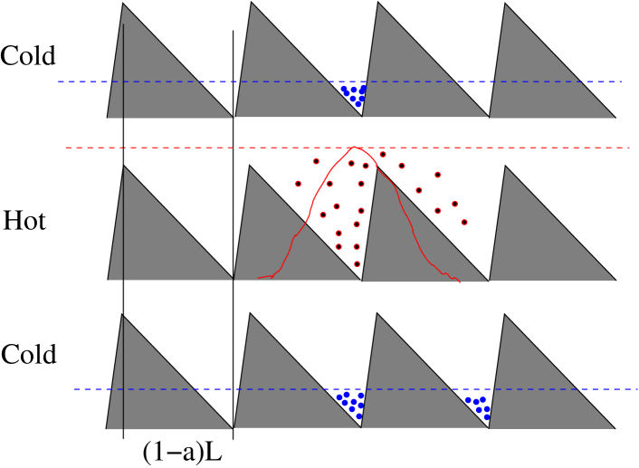
Figure 2. Working principle of a Brownian motor driven by temperature oscillations [19]: Consider suspended noninteracting particles in a viscous medium moving along an asymmetric saw-tooth potential of period $L$ and height $\Delta V$ which are subjected to a temperature that changes in time between the values “hot” and “ cold” , $T\in[T_{\rm cold},T_{\rm hot}]$. For simplicity, let $\Delta V/(k_{B}T_{\rm hot})\ll 1$, and $\Delta V/(k_{B}T_{\rm cold})\gg 1$. The dashed line in the middle panel indicates the level $2k_{B}T$ below which circa 95 % of the particles are found at any given time. Initially, when the temperature is cold, the particles are pinned at a potential minimum. Then, when the temperature is switched to “hot”, the particles effectively do not feel the potential and begin to diffuse. In the middle illustration the thin red line indicates a Gaussian-like shape for the corresponding particle distribution. When the temperature is low again, any particles that have diffused the short distance $L_{1}=aL$, with $a<1/2$, to the right are caught in the well to the right; likewise, any particles that have diffused the long distance $L_{2}=(1-a)L$ towards the left are caught in the well to the left, and the rest are pinned again in the original well from which they started out. Because the chance for a particle to diffuse over the short distance $L_{1}$ during the time when the temperature is high is much larger than the chance to diffuse over the long distance $L_{2}$, a net motion to the right is induced by such cyclic temperature fluctuations.

In the case of a static tilted Brownian motor with a fixed temperature $T$, we immediately see that for a given force, say $F<0$, the particle will on average move “downhill”, i.e. $\langle\dot{x}\rangle<0$. This fact holds true for any fixed, non-zero value of the temperature $T$. Returning to the temperature ratchet with $T$ being subjected to periodic, temporal variations, one should expect that the particles still move “downhill” on the average. The numerically calculated corresponding “load curve” (see Fig. 2 in [21]) demonstrates, however, that the opposite is true within an entire interval of negative bias values $F$: Surprisingly indeed, the particles are climbing “uphill” on the average, thereby performing work against the load force $F$. This upward directed motion is apparently triggered by no other source than the thermal fluctuations $\xi(t)$. This key finding is just what is commonly referred to as the Brownian motor effect [16, 21].

Because the average particle current $\langle\dot{x}\rangle$ depends continuously on the load force $F$, it is sufficient for a qualitative analysis to consider the case $F=0$: the occurrence of the Brownian motor or ratchet effect is then tantamount to a finite current

$$\langle\dot{x}\rangle\not=0\ \ \ \mbox{for}\ \ \ F=0\ ,$$ (8)

i.e., the unbiased Brownian motor implements a directed motion of particles.

2.1. Working principle of a Brownian motor

In order to understand the basic physical mechanism behind the ratchet effect at $F=0$, we focus on very strong, i.e. $|A|\lesssim 1$ but adiabatically slow, periodic two-state temperature modulations from (7). During a first time interval, say $t\in[{\cal T}/2,{\cal T}]$, the thermal energy $k_{B}T(t)$ is kept at a constant value $k_{B}{T}\,(1-A)$ much smaller than the potential barrier $\Delta V$ between two neighboring local minima of $V(x)$. Thus, all particles will have accumulated in a close vicinity of the potential minima at the end of this time interval, as sketched in the top panel of Fig. 2. Then, the thermal energy jumps to a value $k_{B}{T}\,(1+A)$ much larger than $\Delta V$ and remains stable during another half period, say $t\in[{\cal T},3{\cal T}/2]$. Because the particles then barely feel the potential profile in comparison to the intense noise level, the particles spread out subject to free thermal diffusion – see Fig. 2, middle panel. Finally, $T(t)$ jumps back to its original “cool” value ${T}\,(1-A)$ and the particles slide downhill towards the closest local minima of $V(x)$. Due to the lack of reflection symmetry of the function $V(x)$, the original population of one given potential well is thus re-distributed asymmetrically, yielding a net average displacement after one temporal period ${\cal T}$.

When the temperature is varied very slowly during a cycle (and restricting the discussion to the case that the potential $V(x)$ has only one minimum and maximum per period $L$, like in Fig. 2) it is quite obvious that if the local minimum is closer to its adjacent maximum located to the right, a positive particle current $\langle\dot{x}\rangle>0$ will arise. Put differently, upon inspection of Fig. 2, it is intuitively clear that during the cool-down cycle the particles must diffuse a long distance to the left, but only a short distance to the right. This in turn induces a net transport against the steeper potential slope towards the right. All these predictions rely on our assumptions that ${T}\,(1\mp A)$ are much smaller/larger than $\Delta V$, and that the time-period $\cal T$ is sufficiently large.

The Brownian motor effect (8) occurs for very general temperature modulations $T(t)$, as well. For the same reason, the ratchet effect is also robust with respect to modifications of the potential shape [19] and is recovered even for random instead of deterministic modulations of $T(t)$ [22], with a modified dynamics on a discrete state space [23], and in the presence of finite inertia [24].

The directed particle current is clearly bound to vanish in the so termed adiabatic limit (i.e. for asymptotically, very slow temperature modulations), when thermal equilibrium is approached. A similar conclusion holds true for asymptotically fast temperature modulations. By use of a correspondent, perturbative Floquet analysis one finds the noteworthy result that the current decays to zero in both asymptotic regimes remarkably fast, namely like ${\cal T}^{-2}$ in the slow modulation limit, and ${\cal T}^{2}$, in the fast modulation limit, respectively [19].

Moreover, for non-adiabatic temperature variations, the Brownian motion in a diffusive Brownian motor moving on a tailored ratchet profile is generally not rectified in its “natural” direction, but rather in the opposite direction [19]. This in turn implies a time-scale induced (non-adiabatic) current-reversal: It is this very feature that is required for an efficient separation of particles of different size, or other transport qualifiers such as friction, mass, etc..

2.2. Features of a Brownian motor

We cannot emphasize enough that the ratchet effect, as exemplified in the temperature Brownian motor model shown in Fig. 2, is not in contradiction with the second law of thermodynamics: the temperature changes in (7) are caused by two heat environments at two different temperatures with which the Brownian motor system is in continuous contact. From this viewpoint, this archetype Brownian motor is nothing else than an extremely simple, small heat engine. The fact that such a device can produce work is therefore not a miracle — but it is still very intriguing. The following characteristics are a hallmark of Brownian motors.

2.2.1. Loose-coupling mechanism

Consider the “relevant state variables” $x(t)$ and $T(t)$ of our temperature Brownian motor. In the case of an ordinary heat engine, these two state variables would always cycle through one and the same periodic sequence of events (“working strokes”). Put differently, the evolutions of the state variables $x(t)$ and $T(t)$ would be tightly coupled and almost synchronized.

In clear contrast to this familiar scenario, the relevant state variables of a genuine Brownian motor are loosely coupled: Some degree of interaction is required for the functioning of the Brownian motor, but while $T(t)$ completes one cycle, $x(t)$ may evolve in a very different way. The spatial coordinate $x(t)$ is certainly not slaved by the unbiased modulation of the temperature $T(t)$.

This loose coupling between state variables is a salient feature of a Brownian motor device and distinguishes the Brownian motor concept from micron-sized, but otherwise quite conventional thermo-mechanical or even purely mechanical engines. In particular, indispensable ingredients of any genuine Brownian motor are: (i) the presence of some amount of (not necessarily thermal) noise; (ii) some sort of symmetry-breaking supplemented by temporal periodicity (possibly via an unbiased, non-equilibrium forcing), if a cyclically operating device is involved. It is thus not appropriate to advertise every such small ratchet device under the trendy label of “Brownian motor”. This holds true especially if the governing transport principle is deterministic, like in mechanical ratchet devices of macro- or mesoscopic size, such as a ratchet wrench, interlocked mechanical gears, or Leonardo’s “cochlea” [25] and other “screw-like” pumping and propulsion devices. By the way, it is suggestive to notice how Leonardo sketched a ratchet-like machinery just to prove the impossibility of the perpetuum mobile [26].

2.2.2. Dominant role of noise

Yet another distinguishing feature of a Brownian motor is that noise (no matter what its source, i.e. stochastic, or chaotic, or thermal) plays a non-negligible, or even a dominant role. In particular, it is the intricate interplay among nonlinearity, noise-activated escape dynamics and non-equilibrium driving which implies, that, generally, not even the direction of transport is a priori predictable. See also in Sects. 4 and 5 below.

2.2.3. Necessary ingredients and variations of the Brownian motor scheme

The necessary condition for the Brownian motor effect is to operate away from thermal equilibrium, namely, in a state with no detailed balance. This was achieved above through the cyclic variation of the temperature (7); but there clearly exists a great variety of other forms of non-equilibrium perturbations [27]. The following guiding prescriptions should be observed when designing a more general Brownian motor:

• Spatial and/or temporal periodicity critically affect rectification.

• All acting forces and gradients must vanish after averaging over space, time, and statistical ensembles.

• Random forces (of thermal, non-thermal, or even deterministic origin) assume a prominent role.

• Detailed balance symmetry must be broken by moving the system away from thermal equilibrium.

• A symmetry-breaking must apply.

There exist several possibilities to induce symmetry-breaking. First, the spatial inversion symmetry of the periodic system itself may be broken intrinsically; that is, already in the absence of non-equilibrium perturbations. This is the most common situation and typically involves a type of periodic asymmetric (so-called ratchet) potential. A second option consists in the use of a deterministic, unbiased skew forcing $f(t)$. For example, these may be stochastic fluctuations $f(t)$ possessing non-vanishing, higher order odd multi-time moments — notwithstanding the requirement that they must be unbiased, i.e. the first moment vanishes [28]. Such an asymmetry can also be created by unbiased periodic non-equilibrium perturbations $f(t)$. Both variants in turn induce a spatial asymmetry of the dynamics. Yet a third possibility arises via a collective effect in coupled, perfectly symmetric non-equilibrium systems, namely in the form of spontaneous symmetry breaking [29, 30, 31]. Note that in the latter two cases we speak of a Brownian motor dynamics even though a ratchet-potential is not necessarily involved. An instructive demo java applet of a Brownian motor can be found on the web [32].

In the next section we shall illustrate this concept for the case of a temporal, dynamical symmetry breaking. This approach is readily implemented experimentally, and therefore does carry a great potential for novel applications and devices.

3. Brownian motors and dynamical symmetry breaking

What we call a ratchet mechanism is to some extent a matter of taste. Our bona fide ratchet prescriptions in Sec. 2.2 apply indeed to a number of diverse microscopic rectification mechanisms that have been known for a long time, well before the notion of Brownian motor became popular. Such mechanisms do involve ingredients like spatial periodicity, random forces, non-equilibrium (detailed balance breaking) and zero-mean external biases (both in space and time). However, in this category of processes the reflection asymmetry of the substrate plays no essential role, although its presence may add certain sofar unnoticed similarities with the ratchet phenomenology. A common feature of all these non-ratchet, or possibly ratchet-related, rectification mechanisms is some degree of temporal synchronization between input signal(s) and/or spatial modulation of the substrate, leading to a dynamical symmetry breaking.

3.1. Harmonic mixing

A charged particle spatially confined by a nonlinear force is capable of mixing two alternating input electric fields of angular frequencies $\Omega_{1}$ and $\Omega_{2}$, its response containing all possible higher harmonics of $\Omega_{1}$, $\Omega_{2}$ and their sum and difference frequencies. For commensurate input frequencies, i.e., $m\Omega_{1}=n\Omega_{2}$, there appears a rectified output component, too [33]: such a dc harmonic mixing (HM) signal is an $(n+m)$-th order effect in the dynamical parameters of the system [34, 35].

Let us consider the stochastic dynamics of an overdamped particle with coordinate $x(t)$,

$$\dot{x}=-V^{\prime}(x)+F(t)+\xi(t),$$ (9)

moving on the one dimensional substrate potential $V(x)=q(1-\cos x)$, subjected to an external zero-mean Gaussian noise $\xi(t)$ with the auto-correaltion function $\langle\xi(t)\xi(0)\rangle=2D\delta(t)$, and a periodic two-frequency drive force

$$F(t)=A_{1}\cos(\Omega_{1}t+\phi_{1})+A_{2}\cos(\Omega_{2}t+\phi_{2}),$$ (10)

with $\Omega_{1}$ and $\Omega_{2}$ integer-valued multiples of the fundamental frequency $\Omega_{0}$, i.e., $\Omega_{1}=n\Omega_{0}$ and $\Omega_{2}=m\Omega_{0}$. For $D=k_{B}T$ the Langevin equation (9) is the zero-mass limit of Eq. (1) with $\eta=1$; in the case of bistable potentials it describes a well-known synchronization phenomenon known as Stochastic Resonance, both in physics [36] and biology [37]. A standard perturbation expansion leads to a general expression [34] for the non-vanishing dc component $j_{0}\equiv\langle\dot{x}\rangle$ of the particle velocity. In the regime of low temperature, $D\ll\Delta V=2q$, the particle net current can be approximated to

$$\frac{j_{0}}{D}=-\frac{\pi^{2}}{2^{m+n}}\left(\frac{A_{1}}{D}\right)^{m}\left(\frac{A_{2}}{D}\right)^{n}\cos(n\phi_{2}-m\phi_{1})$$ (11)

for $\Omega_{0}^{2}\ll q$ (low frequency limit), and to

$$\frac{j_{0}}{\Omega_{0}}=-\frac{1}{2^{m+n}}\left(\frac{q}{D}\right)^{2}\left(\frac{A_{1}}{\Omega_{1}}\right)^{m}\left(\frac{A_{2}}{\Omega_{2}}\right)^{n}\cos(n\phi_{2}-m\phi_{1})$$ (12)

for $\Omega_{0}^{2}\gg q$ (high frequency limit). The sign of $j_{0}$ is controlled by the input phases $\phi_{1}$, $\phi_{2}$, while an average over $\phi_{1}$ or $\phi_{2}$ would eliminate the rectification effect completely. The two sinusoidal components of $F(t)$ get coupled through the anharmonic terms of the substrate potential $V(x)$ [38]; the dependence of $j_{0}$ on $\Delta_{m,n}=n\phi_{2}-m\phi_{1}$ characterizes HM indeed as a synchronization effect.

In the derivation of Eqs. (11) and (12) no assumption was made regarding the reflection symmetry of $V(x)$; actually, HM rectification may occur on symmetric substrates, too. However, a simple perturbation argument [39] leads to the conclusion that a symmetric device cannot mix low-frequency rectangular waveforms, namely no HM is expected for

$$F(t)=A_{1}\hbox{sgn}[\cos(\Omega_{1}t+\phi_{1})]+A_{2}\hbox{sgn}[\cos(\Omega_{2}t+\phi_{2})],$$ (13)

with $A_{1},A_{2}\geq 0$ and $\hbox{sgn}[\dots]$ denoting the sign of $[\dots]$. However, an asymmetric device can!

In order to illustrate the properties of asymmetric HM [40] let us consider the driven dynamics (9) in the piecewise linear potential $V(x)=x\Delta V/L_{2}$ for $-L_{2}<x<0$ and $V(x)=x\Delta V/L_{1}$ for $0<x<L_{1}$, with $L_{1}+L_{2}=L$ and, say, $L_{2}<L_{1}$, i.e. opposite polarity with respect to the potential in Fig. 2; the external drive $F(t)$, in Eq. (13), is assumed to vary slowly in time.

The advantage of imposing the adiabatic limit $\Omega_{1}$, $\Omega_{2}\rightarrow 0$, is that the output $j(\Omega_{1},\Omega_{2},A_{1},A_{2})$ of a such doubly-rocked ratchet is expressible analytically in terms of the current $j_{R}(A)$ of the standard one-frequency rocked ratchet [41], obtained by setting $A_{1}=A$ and $A_{2}=0$ in Eq. (13). Note that here $j_{R}(A)$ is a symmetric function of $A$, and in the adiabatic approximation $j_{R}(A)=j_{R}(-A)=A[\mu(A)-\mu(-A)]/2$, where $\mu(A)$ is the mobility of an overdamped particle running down the tilted potential $V(x)-Ax$.

The overall ratchet current $j(\Omega_{1},\Omega_{2},A_{1},A_{2})$ results from the superposition of the two standard one-frequency currents $j_{R}(A_{1}+A_{2})$ and $j_{R}(A_{1}-A_{2})$ for drive ac amplitudes $A_{1}+A_{2}$ and $A_{1}-A_{2}$, respectively [40]. In particular, for any positive integers $m$, $n$ with $m>n$,

$$j(\Omega_{1},\Omega_{2}=\Omega_{1}\frac{2m-1}{2n-1},A_{1},A_{2}) = j_{\rm avg}(A_{1},A_{2})$$ (14)

$$-{{(-1)^{m+n}}\over{(2m-1)(2n-1)}}~{}\Delta j(A_{1},A_{2})~{}p(\Delta_{n,m}),$$

where

$$j_{\rm avg}(A_{1},A_{2})=\frac{1}{2}[j_{R}(A_{1}-A_{2})+j_{R}(A_{1}+A_{2})]\;,$$

$$~{}~{}~{}~{}\Delta j(A_{1},A_{2})=\frac{1}{2}[j_{R}(A_{1}-A_{2})-j_{R}(A_{1}+A_{2})],$$ (15)

and $p(\Delta_{n,m})={|\pi-\Delta_{n,m}|}/{\pi}-0.5$ is a modulation factor with $\Delta_{n,m}=(2n-1)\phi_{2}-(2m-1)\phi_{1}$, mod($2\pi$).

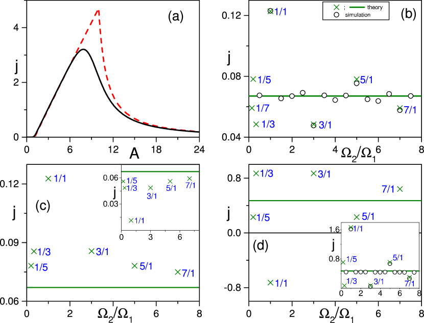
Figure 3. Rectified current driven by two rectangular waveforms with fixed amplitudes: (a) one-frequency rocked ratchet; (b), Harmonic mixing case of Eqs. (9), (10); (d) gating mechanism (16). Panel (a): Response curve $j_{R}(A)$ of the potential $V(x)$ driven by a low-frequency rectangular force with amplitude $A$ at zero temperature $D=0$ (dashed curve), and low temperature $D/\Delta V=0.05$ (solid curve). Panel (b): Numerical simulations for a doubly rocked ratchet with $\phi_{1}=\phi_{2}=\pi$ and $\Omega_{1}=0.01$ (open circles) and in adiabatic approximation (green line and green crosses). The baseline $j_{\rm avg}$, Eq. (3.1), is indicated by the green line; the spikes at some selected integer-valued odd harmonics are marked with green crosses ($\times$); Panel (c): Adiabatic approximation for $\phi_{1}=\phi_{2}=3\pi/2$ (main panel) and $\phi_{1}=3\pi/2$, $\phi_{2}=\pi/2$ (inset). In both cases $A_{1}=3$, $A_{2}=2$, $D=0.6$; Panel (d): Numerical simulations for a rocked-pulsated ratchet in the adiabatic regime with $A_{1}=4$, $A_{2}=0.5$ and $\Omega_{1}=0.01$; noise level: $D=0.4$. Main panel: $\phi_{1}=\phi_{2}=\pi$ (adiabatic approximation); inset: simulation (open circles) versus the fully adiabatic approximation ($\times$) for $\phi_{1}=\pi$ and $\phi_{2}=0$. $V(x)$ parameters are: $L_{1}=0.9$, $L=1$, $\Delta V=1$ in (a)-(c) and $\Delta V=2$ in (d).

The most significant properties of the rectification current (14) and (3.1) are elucidated in Fig. 3(a), (b), where results from numerical simulation are displayed for a comparison [40]: (1) The doubly rocked ratchet current in the adiabatic limit) is insensitive to $\Omega_{1}$, $\Omega_{2}$ for $\Omega_{2}\neq\Omega_{1}=(2m-1)/(2n-1)$; its intensity coincides with the “baseline” value $j_{\rm avg}(A_{1},A_{2})$ of Eq. (3.1); spikes correspond to odd fractional harmonics; their amplitude $\Delta j(A_{1},A_{2})/(2m-1)(2n-1)$ is suppressed at higher harmonics, i.e., for larger $m,n$. (2) The sign of the spike factor $\Delta j(A_{1},A_{2})$ is sensitive to the signal amplitudes $A_{1}$, $A_{2}$. For instance, if we choose $A_{1}$, $A_{2}$ so that $A_{1}+A_{2}$ and $|A_{1}-A_{2}|$ fall onto the rising (decaying) branch of $j(A)$ in Fig. 3a, then $\Delta j(A_{1},A_{2})$ is negative (positive). (3) The current spikes at $\Omega_{2}/\Omega_{1}=(2m-1)/(2n-1)$ depend on the initial value of $\phi_{1}$, and for a fixed $\phi_{1}$, their amplitude oscillates with $\phi_{2}$ proportional to the modulation factor $p(\Delta_{n,m})$. We remark that the overall sign of our doubly rocked ratchet current is always determined by the polarity of $V(x)$ (positive for $L_{2}<L_{1}$), as $|\Delta j(A_{1},A_{2})|<|j_{\rm avg}(A_{1},A_{2})|$ for any choice of $A_{1}$, $A_{2}$. However, in the partially adiabatic regime, where only one frequency tends to zero, multiple current inversions are also possible [40].

3.2. Gating mechanism

A periodically-driven Brownian motion can also be rectified by modulating the amplitude of the substrate potential $V(x)$. Let us consider for instance the overdamped dynamics described by the Langevin equation

$$\dot{x}=-V^{\prime}(x)[1+F_{2}(t)]+F_{1}(t)+\xi(t).$$ (16)

To avoid interference with possible HM effects we follow the prescription of Sec. 3.1, namely we take $F_{i}(t)=A_{i}\hbox{sgn}[\cos(\Omega_{i}t+\phi_{i})]$, with $i=1,2$ and $A_{i}\geq 0$. Mixing of the additive $F_{1}(t)$ and the multiplicative signal $F_{2}(t)$ provides a control mechanism of potential interest in device design. Without loss of generality, our analysis can be conveniently restricted to the piecewise linear potential $V(x)$ also used in the previous subsection.

In the adiabatic limit, the ac driven Brownian particle $x(t)$ can be depicted as moving back and forth over a time modulated potential $V(x,t)=V(x)[1+F_{2}(t)]$ that switches between two alternating configurations $V_{\pm}(x)=V(x)(1\pm A_{2})$. Both substrate profiles $V_{\pm}(x)$ are capable of rectifying the additive driving signal $F_{1}(t)$ with characteristic functions ${j}_{\pm}(A_{1})$, respectively; the net currents ${j}_{\pm}(A_{1})$ are closely related to the curve $j_{R}(A)$ plotted in Fig. 3(a), namely [40]

$${j}_{\pm}(A_{1})=(1\pm A_{2})\,j_{R}\left[\frac{A_{1}}{1\pm A_{2}}\right]\;,$$ (17)

with $D\rightarrow D/(1\pm A_{2})$. It follows that the total net current can be cast in the form (14) with

$$j_{\rm avg}(A_{1},A_{2})=(1/2)[{j}_{-}(A_{1})+{j}_{+}(A_{1})]$$ (18)

and

$$\Delta j(A_{1},A_{2})=(1/2)[{v}_{-}(A_{1})-{v}_{+}(A_{1})],$$ (19)

where $v_{\pm}(A_{1})=A_{1}[\mu_{\pm}(A_{1})+\mu_{\pm}(-A_{1})]/2$. We recall that in our notation $\mu_{\pm}(A)$ is the static nonlinear mobility of the tilted potentials $V_{\pm}(x)-Ax$.

It is apparent that $|\Delta j(A_{1},A_{2})|$ may grow larger than $|j_{\rm avg}(A_{1},A_{2})|$ and, therefore, a current reversal may take place for appropriate values of the model parameters, as shown by the simulation results in Fig. 3(d). In fact, already a relatively small modulation of the ratchet potential amplitude at low temperatures can reverse the polarity of the simply rocked ratchet $V(x)$. Let us consider the simplest possible case, $\Omega_{1}=\Omega_{2}$ and $\phi_{1}=\phi_{2}$: As the ac drive is oriented along the “easy” direction of $V(x)$, namely to the right, the barrier height $V(x,t)$ is set at its maximum value $\Delta V(1+A_{2})$; at low temperatures the Brownian particle cannot overcome this barrier height within a half ac-drive period $\pi/\Omega_{1}$. In the subsequent half period the driving signal $F_{1}(t)$ changes sign, thus pointing against the steeper side of the $V(x,t)$ wells, while the barrier height drops to its minimum value $\Delta V(1-A_{2})$: Depending on the value of $\Delta V/D$, the particle has a better chance to escape a potential well to the left than to the right, thus making a current reversal possible. Of course, the net current may be controlled via the modulation parameters $A_{2}$ and $\phi_{2}$, too (see inset of Fig. 3d).

Note that Eq. (14) is symmetric under $m\leftrightarrow n$ exchange. This implies that, as long as the adiabatic approximation is tenable, each spectral spike $(m,n)$ of the net current is mirrored by a spike $(n,m)$ of equal strength (see Fig. 3). This is not true, e.g., in the partially adiabatic regime, where the dynamics depends critically on which ratio $\Omega_{1}/\Omega_{2}$ or $\Omega_{2}/\Omega_{1}$ tends to zero [40].

The rectification effect introduced in this subsection rests upon a sort of dynamical symmetry breaking mechanism, or synchronized gating, which requires no particular substrate symmetry. In the case of a symmetric piecewise linear potential, $L_{1}=L_{2}$, the baseline current $j_{\rm avg}(A_{1},A_{2})$ clearly vanishes, while the current spikes due to gating remain.

Asymmetry-induced and nonlinearity-induced mixing are barely separable in the case of sinusoidal input signals. This case is analytically less tractable and shows significant differences with respect to the square-wave rectification investigated so far. Spikes in the output current spectrum occur for any rational value of $\Omega_{2}/\Omega_{1}=m/n$, including even fractional harmonics, i.e. $\Omega_{2}/\Omega_{1}=2m/(2n-1)$, or $\Omega_{2}/\Omega_{1}=(2m-1)/2n$, respectively, but they are no longer symmetric under the exchange of $m\leftrightarrow n$. This is so because HM cannot be separated from asymmetry-induced mixing. It has been noticed that a binary mixture of particles [42], diffusing through a quasi-one dimensional channel, provides a convenient study case (both numerical and experimental) to contrast nonlinearity versus asymmetry induced signal mixing.

3.3. Stokes’ drift

Particles suspended in a viscous medium traversed by a longitudinal wave travelling in the $x$-direction, are dragged along according to a deterministic mechanism known as Stokes’ drift [43]. As a matter of fact, the particles spend slightly more time in regions where the force acts parallel to the direction of propagation than in regions where it acts in the opposite direction. Consider [44] a symmetric square wave $f(kx-\Omega t)$ with wavelength $\lambda=2\pi/k$ and temporal period $T_{\Omega}=2\pi/\Omega$, capable of entraining the particles with velocity $\pm bv$ [with $v=\Omega/k$, $0<b<1$, and the signs $\pm$ denoting the orientation of the force]. During one cycle, the particle velocity is positive for a longer time interval, $\lambda/2(1-b)v$, than it is negative, $\lambda/2(1+b)v$; hence, the average drift velocity $v_{S}=b^{2}v$. The unknown factor $b$ depends on the speed of travelling wave $f(kx-\Omega t)$ and the temperature of the propagation medium.

The longitudinal motion of a massive particle on a propagating substrate $V(x,t)$ can be modelled by replacing

$$V(x)\rightarrow V(x,t)=V(x-vt)$$ (20)

in the stochastic differential equation (1). Let us consider first the sinusoidal wave of Fig. 4a

$$V(x,t)=-q\cos(x-vt).$$ (21)

A Galileian transformation, $x(t)\rightarrow y(t)=x(t)-vt$, allows us to reformulate Eq. (1) as [45, 46]

$$m\ddot{y}=-\eta\dot{y}-\eta v-q\sin y+\xi(t).$$ (22)

Equation (22) describes the Brownian motion in the tilted washboard potential $V(y)=-q\cos y+\eta vy$, shown in Fig. 4(b). This problem was studied in great detail by Risken in Ref. [47]. The theme of Brownian motion and diffusion in periodic potentials has also been widely applied to describe the transport properties of superionic conductors [48, 49, 50], or for the evaluation of the thermally activated escape rates and the corresponding current-voltage characteristics of damped Josephson junctions [51, 52]. To make contact with Risken’s notation, we introduce the damping constant $\gamma=\eta/m$, the dc driving force $F=-\gamma v$ and the angular frequency $\omega_{0}^{2}=q/m$. The time evolution of the stochastic process $y(t)$ is characterized by random switches between a locked state with zero-mean velocity and a running state with asymptotic average velocity $\langle\dot{y}\rangle=F/\gamma=-v$. In terms of the mobility $\mu(T)=\langle\dot{y}\rangle/F$, locked and running states correspond to $\gamma\mu=0$ and $\gamma\mu=1$, respectively.

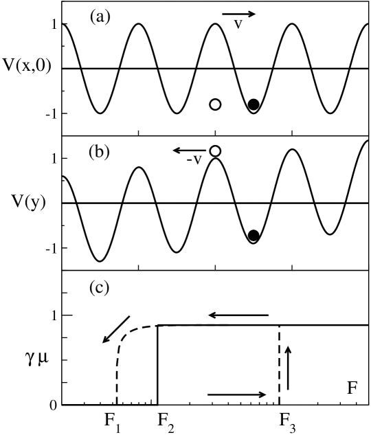
Figure 4. (a) Snapshot of the travelling potential $V(x,t)$ of Eq. (21) at $t=0$. (b) Tilted washboard potential $V(y)$ of Eq. (22). A Brownian surfer is represented by a filled circle, a Brownian swimmer by an empty circle. (c) Locked-to-running state transition for an underdamped Brownian particle in a washboard potential. The dashed curves define the hysteretic loop of the noiseless case $\xi(t)\equiv 0$, with depinning branch starting at $F_{3}=\omega_{0}^{2}$ and re-pinning branch ending at $F_{1}=(4/\pi)\gamma\omega_{0}$ [53]. The $T=0+$ step at $F_{2}$ is represented by a solid curve. Parameter values: $m=q=1$ and $\eta=0.03$.

In the underdamped, $\gamma\ll\omega_{0}$, zero-temperature limit, $T\rightarrow 0$, the stationary dynamics (22) is controlled by a single threshold $F_{2}\simeq 3.36\omega_{0}\gamma$, see Fig. 4c: For $F<F_{2}$ the particle $y(t)$ sits in one potential well; for $F>F_{2}$ it falls down the tilted washboard potential with speed $F/\gamma$; the $0\leftrightarrow 1$ jump of $\gamma\mu(T)$ at the threshold $F_{2}$ becomes sharper as $T$ tends to zero.

On reverting to Eq. (22) notation, we see immediately that the thresholds $F_{1}$-$F_{3}$ in Fig. 4(c) define three special values of the travelling wave $v$, namely:

$$v_{1}=\frac{4}{\pi}\sqrt{\frac{q}{m}},\,\,\,\,\,v_{2}\simeq 3.36\sqrt{\frac{q}{m}},\,\,\,\,\,v_{3}=\frac{q}{\eta}.$$ (23)

Upon equating $v_{1}$ and $v_{3}$ we attain an estimate for the upper limit $\eta_{0}$ of the damping constant below which we may expect to detect a hysteretic cycle, i.e. $\eta_{0}/m=(\pi/4)\sqrt{q/m}$. On increasing $\eta$ much larger than $\eta_{0}$, $v_{1}$ and $v_{2}$ merge with $v_{3}$, which in turn becomes very small [47].

The stationary velocity of the Brownian particle $x(t)$ can be easily determined by inverting the $x\rightarrow y$ transformation, that is

$$v_{S}\equiv\langle\dot{x}\rangle=v[1-\gamma\mu(T)]\equiv b^{2}(T)v,$$ (24)

where $v$ is the velocity of the incoming wave and $b(T)$ is the unknown Stokes’ factor. In the presence of noise, no matter how weak, say $T=0+$, the dynamics of the process is controlled by $v_{2}$, only: For $v>v_{2}$ the process $y(t)$ is in the running state with $\gamma\mu(T)\simeq 1$, or equivalently the particle $x(t)$ is subjected to no Stokes’ drift, i.e., $v_{S}\simeq 0$; for $v<v_{2}$ the process $y(t)$ is in the locked state with $\mu(T)\simeq 0$, which corresponds to a dragging speed $v_{S}\simeq v$ of the Brownian particle $x(t)$. In the latter case the particle rides the travelling wave like a surfer (Brownian surfer [45]).

The efficiency of the Stokes’ drift increases when lowering the temperature. Moreover, in the low damping regime, $\eta\ll\eta_{0}$, it sets on abruptly by tuning the parameters $m$ and $q$ to appropriate threshold values – see Eq. (23). Brownian surfers in the overdamped limit, $\eta\gg\eta_{0}$, are restricted to either extremely low frequencies or exceedingly large amplitudes of the travelling wave, namely $\eta v<q$; for $\eta\rightarrow\infty$ the dragging effect thus becomes less and less efficient.

A massive Brownian particle undergoes Stokes’ rectification in the presence of time and space modulation of its substrate, see also [54]. For the travelling wave (21) the displacement of any point on the substrate averages out to zero, and so does the spatial average of the substrate deformation at a given time $t$. However, if we regard $V(x,t)$ as a propagating elastic wave, the corresponding synchronization of time and space modulations sustains a net energy transport in the direction of propagation. In this sense the dynamics (1) is biased and Stokes’ drift requires no asymmetric profile of the travelling substrate wave.

For an asymmetric waveform $V(x,t)$, Eqs. (1) and (20) describe a travelling ratchet. Asymmetry makes then the Stokes’ drift problem more intriguing. Suppose we propagate the piecewise linear potential $V(x)$ of Sec. 3.1 with constant velocity $v$ according to Eq. (20). Because of the spatial asymmetry, we can define two threshold speeds $v_{2}^{\pm}$ for a wave travelling to the right and to the left, respectively, with $v_{2}^{-}>v_{2}^{+}$. This implies that at low temperatures Stokes’ drift to the right becomes effective e.g. for larger particle masses, viz. lower substrate amplitudes, than to the left.

However, if the substrate oscillates side-wise with a constant speed, with

$$v\rightarrow v(t)=v~{}\hbox{sgn}[\cos(\Omega_{v}t)]$$ (25)

and $\Omega_{v}\ll v/l$, the corresponding moving waveform $V(x,t)$ in average transports no energy, but can still induce rectification because of its asymmetry. Indeed, for $v_{2}^{+}<v<v_{2}^{-}$ the Brownian surfer drifts to the right and the system works like a “massive particle sieve”. Note that in the notation of Eq. (22) such a particle sieve corresponds to a simple inertial rocked-ratchet [24, 55]

4. Quantum Brownian motors

Brownian motors are typically small physical machines which operate far from thermal equilibrium by extracting energy fluctuations, thereby transporting classical objects on the micro-scale. At variance with e.g. biomolecular motors, certain molecular sized physical engines necessitate, depending on temperature and the nature of particles to be transported, a description that accounts for quantum effects, such as quantum tunnelling and reflection in the presence of quantum Brownian motion [56]. For this class of quantum Brownian motors recent theoretical studies [35, 57, 58] have predicted that the transport becomes distinctly modified as compared to its classical counterpart. In particular, intrinsic quantum effects such as tunnelling-induced current reversals [57, 59], power-law-like quantum diffusion transport laws, and quantum Brownian heat engines have been observed with recent, trend-setting experiments that involve either arrays of asymmetric quantum dots [59], or certain cell-arrays composed of different Josephson junctions [60].

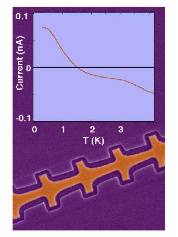
Figure 5. In a quantum Brownian motor, being driven by an adiabatically varying ac-rocking voltage, quantum tunnelling can contribute to the electron current. Due to the underlying asymmetric potential structure, the two components to the time-averaged net current are of opposite sign [57]. The strength of the two contributions can be tuned individually by temperature. This causes a tunnelling-induced current reversal (occurring near $1.5$K in the top graph) [59] that can be exploited to direct electrons along a priori designed routes. Below the measurement graph is a scanning electron micrograph of the used quantum ratchet device. Figure provided by Heiner Linke, University of Oregon.

In contrast to the classical description, the theory for quantum Brownian motors (as well as corresponding experiments) is much more demanding. This is mainly rooted in the fact that one has to master the mutual interplay of (i) quantum mechanics, (ii) quantum dissipation, and (iii) non-equilibrium driving. Any of these three aspects alone is already not straightforward to accommodate theoretically. In particular, the theoretical description of non-equilibrium, dissipative quantum Brownian motors schemes is plagued by difficulties such as: (a) the commutator structure of quantum mechanics occurring in the Hilbert space of the combined system plus the bath(s), (b) the description of quantum dissipation that at all times necessitates consistency with the Heisenberg relation and the entanglement features between system and environment(s), (c) the correct treatment of quantum detailed balance [61] in equilibrium, so that no quantum Maxwell demon is left alive when all applied non-equilibrium sources are “switched-off”, to name only a few of the main causes of possible theory-related pitfalls.

The present state of the art of the theory is thereby characterized by specific restrictions such as, e.g., an adiabatic driving regime, a tight-binding description, a semiclassical analysis, or combinations thereof [57, 58]. As such, the study of quantum Brownian motors is far from being complete and there is plenty of room and an urgent need for further developments. A particular challenge for theory and experiments are quantum Brownian motors that are built from bottom up on the nano-scale. First results for quantum Brownian rectifiers based on infrared irradiated molecular wires have recently been investigated in [62]. In those quantum systems one employs coherent, driven tunnelling [63] through tailored asymmetric nano-structures, in combination with dissipation due the coupling to macroscopic fermionic leads, which are kept at thermal equilibrium.

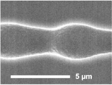
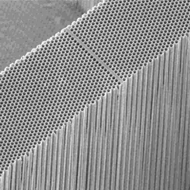
a)  b)

Figure 6. Panel (a): A scanning-electron-microscope picture of a single pore with a ratchet-shaped (i.e., asymmetric) periodic variation of the diameter along its axis; the length of one period is $8.4\mu\text{m}$. Panel (b): Scanning-electron-microscope picture of a silicon wafer which is pierced by a huge number of practically identical pores with pore distances of 1.5 mm and pore diameters of 1 mm. This illustrates the enormous potential for separation with a parallel three-dimensional ratchet-architecture.

As a typical example where theory and experiment have met, we discuss the case of a rocking quantum ratchet as depicted in the bottom panel in Fig. 5. It is known that for a slowly rocked classical Brownian motor (adiabatic regime) [41, 64], the noise-induced transport does not exhibit a reversal of current direction. Such a reversal occurs only in the non-adiabatic rocking regime at higher driving frequencies [41]. This very situation changes drastically when quantum tunnelling enters into the dynamics. A true benchmark for a quantum behavior of an adiabatically rocked Brownian motor is then the occurrence of a tunnelling-induced reversal at low temperatures, as theoretically predicted in [57]. This characteristic feature has been experimentally verified with an electron quantum rocking Brownian motor composed of a two-dimensional gas of electrons moving within a fabricated, ratchet-tailored hetero-structure of a GaAs/AlGaAs interface [59], see the top panel of Fig. 5. This current reversal indicated the existence of parameter configurations where the quantum Brownian motor current vanishes. In the neighborhood of these system configurations we consequently can devise a quantum refrigerator that separates “cold” from “hot” electrons in absence of currents [59].

5. Recent applications

Over the last decade or so, many theoretical schemes and experimental implementations of Brownian motors have been devised [16, 21]. Several recent applications use an external rocking force, of electric or mechanical origin, as a tunable control.

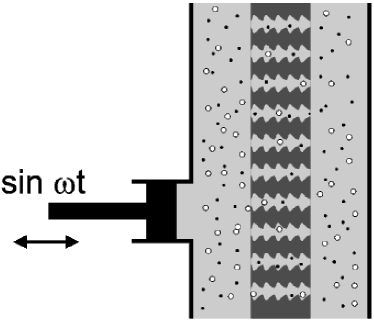
a)  b) .

Figure 7. Panel (a): Concept of a microfluidic drift ratchet. Schematic cross section through the plane of the experimental setup. A macro-porous silicon wafer is connected at both ends to basins. The pores with their ratchet-shaped profile are schematically indicated in dark grey. The basins and the pores are filled with liquid; micrometer-sized particles of two different species are indicated. The fluid is pumped back and forth by a pumping device, indicated by the piston on the left hand side. Figures provided by Christiane Kettner et al. [71]. Panel (b): Average Brownian motor induced particle current $v_{e}$ versus particle diameter for various driving frequencies $\omega/2\pi$ and viscosities (relative to water) $\nu_{R}$. Particularly note the very sharp velocity reversal around $0.5\,\mu$m. For further details, see Kettner et al. [71]

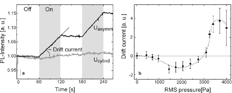
Figure 8. Parallel acting Brownian motors: Asymmetric pores in a macroporous silicon membrane containing ca. 1.7 million pores act as massively parallel Brownian motors, cf. in Ref. [72]. When the pressure oscillations of the water are switched on, the photoluminescence signal and thus the number of particles in the basin located to the right, see in panel (a) of Fig. 7 increases linearly. For symmetrically, cylindrical-shaped pores no systematic drift is observed, see in a). The net transport behavior is strongly dependant on the applied pressure amplitude and shows qualitatively the theoretically predicted current inversion b). The pressure oscillations are toggled on and off each 60 s. The experimental parameters used are as follows: the suspended luminescent polystyrene spheres in water possess a diameter of 0.32 $\mu\text{m}$, the pressure oscillation frequency is 40 Hz and the applied root mean square (r.m.s.) pressure during the ‘on’ phase of 2000 Pa. The number of etched modulations in a single pore was 17. [Image: Max-Planck-Institute of Microstructure Physics]

A few fascinating examples are the light powered single-molecule opto-mechanical cycle, experimentally studied by H. E. Gaub and collaborators [65], the use of colloidal suspensions of ferromagnetic nanoparticles [66], ratchet devices that control the motion of magnetic flux quanta in superconductors [30, 31, 67, 68], or the Brownian motor induced clustering of a vibrofluidized granular gas yielding the phenomenon of a granular fountain and the granular ratchet transport perpendicular to the direction of unbiased energy input [69]. Yet another (Brownian motor)-related phenomenon is the emergence of paradoxical motion of noninteracting, driven Brownian particles exhibiting an absolute negative mobility and corresponding current reversals [70]. Note that an absolute negative mobility implies that the response is opposite to the applied force that is applied around the origin of zero force; as such, this phenomenon must be distinguished from so-called differential negative mobility which is typified by a negative-valued slope of the response-force characteristics away from the origin.

Here, we discuss the prominent potential of a microfluidic realization of Brownian motors that can be used to separate particles with large separation power and in short times. The set-up of the device is depicted in Figs. 6, 7. It consists of a three-dimensional array of asymmetric pores, see Fig. 6a), b) in which a fluid such as water containing some immersed, suspended polystyrene particles is pumped back and forth with no net bias (!), see Fig. 7a). Due to the asymmetry of the pores, the fluid develops, however, asymmetric flow patterns [71], thus providing the ratchet field of force in which a Brownian particle of finite size can both, (i) undergo Einstein diffusion into liquid layers of differing speed, and/or (ii) become reflected asymmetrically from the pore walls. Both mechanisms will then result in a driven non-equilibrium net flow of particles.

The numerical evaluation of the Brownian motor current then yields a rich behavior, featuring an amazingly steep current reversal as a function of the particle size, see Fig. 7b). Note that the direction of the net flow cannot be easily guessed a priori; indeed, the direction of the Brownian motor current is determined by the interplay of the Navier-Stokes flows in this tailored geometry and hydrodynamic thermal fluctuations. This proposal for a microfluidic ratchet-based pumping device has recently been put to work successfully with experiments [72]: the experimental findings are in good qualitative agrement with theory; but more work is required to achieve detailed quantitative agreement.

Remarkably, this device has advantageous three-dimensional scaling properties [71, 73]: a massively parallel architecture composed of ca. 1.7 million pores, cf. Fig. 6b), is capable to direct and separate micron sized suspended objects very efficiently, see in Fig. 8. These type of devices have clear potential for bio-medical separation applications and therapy use.

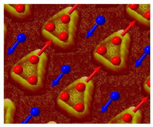
Figure 9. Superconducting Niobium film grown on an array of Nickel triangles. The magnetic flux quanta, or vortices, shown as balls, can be separated in two groups: (i) pinned vortices, shown in red, which move from one triangular-shaped pinning trap to another one and, thus, these are directly affected by the pinning potential; and (ii) interstitial vortices, shown in blue, which move in-between triangles, and do not directly interact with the pinning traps. However, the interstitial vortices can indirectly feel the spatial asymmetry via their interactions with the pinned vortices. This problem can be mapped into the similar system of two species of repulsive particles in which one type or species of particles directly interacts with the spatially-asymmetric substrate. The other type of particle (interstitial vortices here, shown in blue) is insensitive to the substrate, at least in a direct manner. It has been shown in that those particles (assigned red) subject to the substrate potential create an effective asymmetric potential, with the opposite asymmetry or opposite polarity, for the other (blue) particles. When all the particles are subjected to an ac drive force, this “inverted-polarity” potential rectifies the motion of the blue particles (interstitial vortices in our case) in one direction, and the original pinning potential rectifies the motion of the red particles (pinned vortices) along the opposite direction, because the latter feel a potential with opposite polarity. Figure provided by Jose Vicent, Universidad Complutense de Madrid.

Another area of growth regarding applications of Brownian motors to micro-devices involve the control of the motion of quantized flux quanta in superconductors [30, 31, 67, 68]. For instance, the authors of Ref. [68] fabricated a device that controls the motion of flux quanta in a Niobium superconducting film grown on an array of nanoscale triangular pinning potentials, cf. Fig. 9.

The controllable rectification of the vortex motion is due to the asymmetry of the fabricated magnetic pinning centers. The reversal in the direction of the vortex flow is explained theoretically by the interaction between the vortices trapped on the magnetic nanostructures and the interstitial vortices. The applied magnetic field and input current strength can tune both the polarity and magnitude of the rectified vortex flow. That ratchet system is explained and modeled theoretically considering the interactions between particles. This device allows a versatile control of the motion of vortices in superconducting films. Simple modifications and extensions of it [30, 31, 67, 68]would allow the pile-up (magnetic lensing), shaping, or ”sculpting” of micromagnetic profiles inside superconductors. Vortex lenses made of oppositely oriented asymmetric traps would provide a strong local increase of the vortex density at its focus regions. Extensions of these types of systems [30, 31, 67, 68] could allow the motion control of interacting particles in colloidal suspensions, and interacting particles in micro-pores, and not just controlling the motion of flux quanta. These systems provide a step toward the ultimate control of particle motion in tiny microscopic devices.

6. Conclusion

With this work we commemorate some intriguing features of the rich physics of Brownian motion which Albert Einstein pioneered 100 years ago. We can assess that the physics of classical and quantum Brownian motion and its use for technological are still very much under investigation. One main lesson to be learned from Einstein’s work is that rather than fighting thermal Brownian motion we should put it to constructive use: Brownian motors take advantage of this ceaseless noise source to efficiently direct, separate, pump and shuttle particles reliably and effectively.

This work has been supported by the Deutsche Forschungsgemeinschaft, SFB-486, project A-10 (PH); DFG-Sachbeihilfe HA 1517/13-4 (PH); and the Baden-Württemberg-Bayern initiative on quantum information processing (PH). FN acknowledges support from the NSA and ARDA under AFOSR contract No. F49620-02-1-0334 and the NSF grant EIA-0130383.

References

- [1] A. Einstein, Ann. Phys. (Leipzig) 17, 549 (1905).
- [2] A. Einstein, Ann. Phys. (Leipzig) 19, 371 (1906); see also: A. Einstein, Ann. Phys. (Leipzig) 19, 289 (1906); A. Einstein, Z. f. Elektrochemie 14, 235 (1908).
- [3] M. Gouy, J. de Phys. 7 (2), 561 (1888).
- [4] J. Ingen-Housz, Remarks on the use of the microscope (in German), In: Vermischte Schriften phisisch-medizinischen Inhalts [von] J. Ingen-Housz, 2-nd ed., translated and edited by Niklas Karl Molitor, Vol. 2, pp. 122-126 (1784) (C. F. Wappler, Vienna, 1784). The original is in French, in: Nouvelles Expériences Et Observations Sur Divers Objets De Physique par J. Ingen-Housz, 2, pp. 1-5 (1789); printed because of the tardinesss by the publisher only in 1789 (Théophile Barrois, Paris, 1789). An english translation can be found in: P. W. van der Pas, The discovery of the Brownian motion, Scientiarum historia 13, 27-35 (1971). Notably, Jan Ingen-Housz (1730-1799) is also the pioneer of photosynthesis research, see in: H. Gest, Photosyntesis Res. 63, 183-190 (2000).
- [5] R. Brown, Philos. Mag. N. S. 4, 161 (1828); R. Brown, Philos. Mag. N. S. 6, 161 (1829); R. Brown, Ann. Phys. und Chem. (Poggendorff Ann.) 14, 294 (1828); reprinted also in: Edin. New Phil. J. 5, 358 (1828); see also the beautiful historical account on Brownian motion in: R. M. Mazo, Brownian motion (Oxford Science Publisher, Oxford, 2002).
- [6] M. von Smoluchowski, Ann. Phys. (Leipzig) 21, 756 (1906).
- [7] T. N. Thiele, Sur la compensation de quelques erreurs qausi-systématiques par la méthodes de moindre carrées (Reitzel, Copenhagen, 1880); see also: A. Hald, T. N. Thiele’scontributions to statistics, Int. Stat. Rev. 49, 1 (1981).
- [8] L. Bachelier, Annales Scientifiques de l’École Normale Supérieure, Sup. III, 17, 21 (1900); L. Bachelier, Théorie de la Spéculation, (Gauthiers-Villars, Paris 1900; reprinted by: Éditions Jaques Gabay, Paris, 1995).
- [9] Lord Rayleigh, Philos. Mag 32, 424 (1891); Lord Rayleigh, In: Scientific Papers of Lord Rayleigh, Vol. III, (Dover, New York, 1964), p. 471.
- [10] A. Einstein, Z. f. Elektrochemie 13, 41 (1907).
- [11] S. Exner, Wiener Sitzungsber. 56, 116 (1867).
- [12] F. Exner, Ann. Phys. (Leipzig) 2, 843 (1900).
- [13] J. Perrin, Comptes Rendues Acad. Sci. Paris 158, 1168 (1914).
- [14] H. B. Callen and T. A. Welton, Phys. Rev. 83, 34 (1951); R. Kubo, J. Phys. Soc. Japan 12, 570 (1957); R. Kubo, J. Phys. Soc. Japan 17, 1100 (1962).
- [15] The term Brownian motor was first coined by one of us in: R. Bartussek and P. Hänggi, Physikalische Blätter 51 (No. 6), 506 (1995).
- [16] P. Hänggi and R. Bartussek, Lect. Notes Phys. 476, 294 (1996); R. D. Astumian, Science 276, 917 (1997); R. D. Astumian and P. Hänggi, Physics Today 55 (No.11), 33 (2002); P. Reimann, Phys. Rep. 361, 57 (2002); H. Linke, Appl. Phys. A 75, 167 (2002).
- [17] H. S. Leff and A. R. Rex, Maxwell’s demon, Entropy, Information, Computing (Adam Hilger, Bristol, 1990).
- [18] F. Jülicher, A. Ajdari, J. Prost, Rev. Mod. Phys. 69, 1269 (1997); E. Frey, ChemPhysChem 3, 270 (2002); J. Howard, Mechanics of Motor Proteins and the Cytoskeleton (Sinauer Assoc., Sunderland, 2001).
- [19] P. Reimann, R. Bartussek, R. Häussler, and P. Hänggi, Phys. Lett. A 215, 26 (1996).
- [20] P. Hänggi and H. Thomas, Phys. Rep. 88, 207 (1982); note section 4 therein, in particular pp. 264–275.
- [21] P. Reimann and P. Hänggi, Appl. Phys. A 75, 169 (2002).
- [22] J. Luczka, T. Czernik, and P. Hänggi, Phys. Rev. E 56, 3968 (1997); Y.-X. Li, Physica A 238, 245 (1997); I. Zapata, J. Luzcka, F. Sols, and P. Hänggi, Phys. Rev. Lett. 80, 829 (1998); J. D. Bao and S. J. Liu, Phys. Rev. E 60, 7572 (1999).
- [23] M. I. Sokolov and A. Blumen, J. Phys. A 30, 3021 (1997); M. I. Sokolov and A. Blumen, Chem. Phys. 235, 39 (1998).
- [24] J.-D. Bao, Phys. Lett. A 267, 122 (2000).
- [25] Leonardo da Vinci, Codex Atlanticus, sh. 1069r (1478-1518), Biblioteca Ambrosiana, Milan, Italy.
- [26] Leonardo da Vinci, Codex Forster II, sh. 90v (1495-1497).
- [27] A. Ajdari and J. Prost, Comptes Rendues Acad. Sci. Paris 315 (Sér. II), 1635 (1992); R. D. Astumian and M. Bier, Phys. Rev. Lett. 72, 1766 (1994); C. R. Doering, W. Horsthemke, J. Riordan, Phys. Rev. Lett. 72, 2984 (1994); R. Bartussek, P. Reimann, and P. Hänggi, Phys. Rev. Lett. 76, 1166 (1996).
- [28] P. Hänggi, R. Bartussek, P. Talkner, and J. Luczka, Europhys. Lett. 35, 315 (1996); J. Luzcka, R. Bartussek, and P. Hänggi, Europhys. Lett. 31, 431 (1995).
- [29] F. Jülicher and J. Prost, Phys. Rev. Lett. 75, 2618 (1995); F. Marchesoni, Phys. Rev. Lett. 77, 2364 (1996); Z. Csahók, F. Family, and T. Vicsek, Phys. Rev. E 55, 5179 (1997); Z. Zheng, B. Hu, and G. Hu, Phys. Rev. E 58, 7085 (1998); P. Reimann, R. Kawai, C. van den Broeck, and P. Hänggi, Europhys. Lett. 45, 545 (1999) (see also the demo applet http://www.kawai.phy.uab.edu/research/motor/).
- [30] J. F. Wambaugh, C. Reichhardt, C. J. Olson, F. Marchesoni, and F. Nori, Phys. Rev. Lett. 83, 5106 (1999); C. J. Olson, C. Reichhardt, B. Jankó, and F. Nori, Phys. Rev. Lett. 87, 177002 (2001);
- [31] S. Savel’ev, F. Marchesoni, and F. Nori, Phys. Rev. Lett. 91, 10601 (2003); B. Y. Zhu, F. Marchesoni, V. V. Moshchalkov, and F. Nori, Phys. Rev. B 65, 14514 (2003); B. Y. Zhu, F. Marchesoni, V.V. Moshchalkov, and F. Nori, Physica C 388, 665 (2003); B. Y. Zhu, F. Marchesoni, and F. Nori, Physica E 18, 318 (2003); F. Marchesoni, B.Y. Zhu, and F. Nori, Physica A 325, 78 (2003); B.Y. Zhu, F. Marchesoni, and F. Nori, Phys. Rev. Lett. 92, 180602 (2004).
- [32] see: http://monet.physik.unibas.ch/~elmer/bm/
- [33] W. Schneider and K. Seeger, Appl. Phys. Lett. 8, 133 (1966).
- [34] F. Marchesoni, Phys. Lett. A 119, 221 (1986).
- [35] I. Goychuk and P. Hänggi, Europhys. Lett. 43, 503 (1998).
- [36] L. Gammaitoni, P. Hänggi, P. Jung, and F. Marchesoni, Rev. Mod. Phys. 70, 223 (1998).
- [37] P. Hänggi, ChemPhysChem 3, 285 (2002).
- [38] H. J. Breymayer and W. Wonneberger, Z. Phys. B 43, 329 (1981).
- [39] L. D. Landau and E. M. Lifshitz, Mechanics (Butterworth-Heinemann, New York, 1976), ch. 5.
- [40] S. Savel’ev, F. Marchesoni, P. Hänggi, and F. Nori, Europhys. Lett. 67, 179 (2004); S. Savel’ev, F. Marchesoni, P. Hänggi, and F. Nori, Phys. Rev. E 70, 066109 (2004); S. Savel’ev, F. Marchesoni, P. Hänggi, and F. Nori, European Physics Journal B 40, 403 (2004).
- [41] R. Bartusek, P. Hänggi, and J. G. Kissner, Europhys. Lett. 28, 459 (1994).
- [42] S. Savel’ev, F. Marchesoni, and F. Nori, Phys. Rev. Lett. 92, 160602 (2004).
- [43] G. G. Stokes, Trans. Cambridge Philos. Soc. 8, 441 (1847).
- [44] C. Van den Broeck, Europhys. Lett. 46, 1 (1999).
- [45] M. Borromeo and F. Marchesoni, Phys. Lett. A 249, 199 (1998).
- [46] F. Marchesoni and M. Borromeo, Phys. Rev. B 65, 184101 (2002).
- [47] H. Risken, The Fokker-Planck equation (Springer, Berlin, 1984), ch. 11.
- [48] P. Fulde, L. Pietronero, W. R. Schneider, and S. Strässler, Phys. Rev. Lett. 35, 1776 (1975); W. Dieterich, I. Peschel, and W. R. Schneider, Z. Physik B 27, 177 (1977); T. Geisel, Sol. State Commun. 32, 739 (1979).
- [49] W. Dieterich, P. Fulde, and I. Peschel, Adv. Phys. 29, 527 (1980).
- [50] T. Geisel, Topics in Current Physics (Springer, Berlin, 1979) Vol. 15, ch. 8, pp: 201-248.
- [51] P. Hänggi, P. Talkner, and M. Borkovec, Rev. Mod. Phys. 62, 251 (1990); see section 7B therein.
- [52] R. L. Stratonovich, Radiotekhnika i elektronika 3 (No. 4), 497 (1958); V. I. Tikhonov, Avtomatika i telmekhanika 20 (No. 9), 1188 (1959); R. L. Stratonovich, Topics in the Theory of Random Noise, Vol. II (Gordon and Breach, New York-London, 1967); Yu. M. Ivanchenko and L. A. Zil’berman, Zh. Eksp. Teor. Fiz 55 2395 (1968) [Sov. Phys. JETP 28, 1272 (1969)]; V. Ambegaokar and B. I. Halperin, Phys. Rev. Lett. 22, 1364 (1969); H. Grabert, G.-L. Ingold, and B. Paul, Europhys. Lett. 44, 360 (1998).
- [53] M. Borromeo, G. Costantini, and F. Marchesoni, Phys. Rev. Lett. 82, 2820 (1999)
- [54] M. Borromeo and F. Marchesoni, Appl. Phys. Lett. A 75, 1024 (1999).
- [55] F. Marchesoni, Phys. Lett. A 237, 126 (1998).
- [56] H. Grabert, P. Schramm, and G. L. Ingold, Phys. Rep. 168, 115 (1988).
- [57] P. Reimann, M. Grifoni, and P. Hänggi, Phys. Rev. Lett. 79, 10 (1997); P. Reimann and P. Hänggi, Chaos 8, 629 (1998).
- [58] I. Goychuk, M. Grifoni, and P. Hänggi, Phys. Rev. Lett. 81, 649 (1998); I. Goychuk, M. Grifoni, and P. Hänggi, Phys. Rev. Lett. 81, 2837 (1998); M. Grifoni, M. S. Ferreira, J. Peguiron, and J. B. Majer, Phys. Rev. Lett. 89, 146801 (2002); S. Scheidl and V. M. Vinokur, Phys. Rev. B 65, 195305 (2002); L. Machura, M. Kostur, P. Hänggi, P. Talkner, and J. Luczka, Phys. Rev. E 70, 031107 (2004).
- [59] H. Linke, T. E. Humphrey, and A. Lofgren, Science 286, 2314 (1999); H. Linke, T. E. Humphrey, and P. E. Lindelof, Appl. Phys. A 75, 237 (2002); T. E. Humphrey, R. Newbury, R. P. Taylor, and H. Linke, Phys. Rev. Lett. 89, 116801 (2002).
- [60] J. B. Majer, J. Peguiron, M. Grifoni, M. Tusveld, and J. E. Mooij, Phys. Rev. Lett. 90, 056802 (2003).
- [61] P. Talkner, Ann. Phys. (New York) 167, 390 (1986).
- [62] J. Lehmann, S. Kohler, P. Hänggi, and A. Nitzan, Phys. Rev. Lett. 88, 228305 (2002); J. Lehmann, S. Kohler, P. Hänggi, and A. Nitzan, J. Chem. Phys. 118, 3283 (2003).
- [63] M. Grifoni and P. Hänggi, Phys. Rep. 304, 229 (1998).
- [64] M. O. Magnasco, Phys. Rev. Lett. 71, 1477 (1993).
- [65] T. Hugel, N. B. Holland, A. Cattani, L. Moroder, M. Seitz, and H. E. Gaub, Science 296, 1103 (2002).
- [66] A. Engel, H. W. Müller, P. Reimann, and A. Jung, Phys. Rev. Lett. 91, 060602 (2003); M. I. Shliomis, Phys. Rev. Lett. 92, 188901 (2004); A. Engel and P. Reimann, Phys. Rev. Lett. 92, 188902 (2004).
- [67] S. Savel’ev and F. Nori, Nature Materials 1, 179 (2002).
- [68] J. E. Villegas, S. Savel’ev, F. Nori, E. M. Gonzales, J. V. Anguita, R. Garcia, and J. L. Vicent, Science 302, 1188 (2003).
- [69] D. van der Meer, P. Reimann, K. van der Weele, and D. Lohse, Phys. Rev. Lett. 92, 184301 (2004).
- [70] R. Eichhorn, P. Reimann, and P. Hänggi, Phys. Rev. Lett. 88, 190601 (2002); R. Eichhorn, P. Reimann, and P. Hänggi, Phys. Rev. E 66, 066132 (2002); R. Eichhorn, P. Reimann, P. Hänggi, Physica A 325, 101 (2003).
- [71] C. Kettner, P. Reimann, P. Hänggi, and F. Müller, Phys. Rev. E 61, 312 (2000).
- [72] S. Matthias and F. Müller, Nature 424, 53 (2003).
- [73] F. Müller, A. Birner, J. Schilling, U. Gösele, C. Kettner, and P. Hänggi, Phys. Stat. Sol. (a) 182, 585 (2000).