Persistence in systems with conserved order parameter

Abstract

We consider the low-temperature coarsening dynamics of a one-dimensional Ising ferromagnet with conserved Kawasaki-like dynamics in the domain representation. Domains diffuse with size-dependent diffusion constant, $D(l)\propto l^{\gamma}$ with $\gamma=-1$. We generalize this model to arbitrary $\gamma$, and derive an expression for the domain density, $N(t)\sim t^{-\phi}$ with $\phi=1/(2-\gamma)$, using a scaling argument. We also investigate numerically the persistence exponent $\theta$ characterizing the power-law decay of the number, $N_{p}(t)$, of persistent (unflipped) spins at time $t$, and find $N_{p}(t)\sim t^{-\theta}$ where $\theta$ depends on $\gamma$. We show how the results for $\phi$ and $\theta$ are related to similar calculations in diffusion-limited cluster-cluster aggregation (DLCA) where clusters with size-dependent diffusion constant diffuse through an immobile ‘empty’ phase and aggregate irreversibly on impact. Simulations show that, while $\phi$ is the same in both models, $\theta$ is different except for $\gamma=0$. We also investigate models that interpolate between symmetric domain diffusion and DLCA.

I Introduction

Phase separation in the one-dimensional Ising ferromagnet is a well-understood phenomenon bray94 ; derrida94 ; derrida95 . At zero temperature, with Glauber (nonconserved) dynamics, coarsening occurs through the irreversible annihilation of domain walls, and the mean domain size grows as $L(t)\sim t^{1/2}$. The coarsening process is equivalent to the diffusion-limited single-species annihilation reaction $A+A\rightarrow 0$, where $A$ particles represent domain walls. Although no simple particle model can be constructed for Kawasaki (spin-exchange) dynamics due to the nearest-wall correlations introduced by the conservation principle, qualitatively similar coarsening dynamics kinetics (but with a different domain-growth law, $L(t)\sim t^{1/3}$) have been observed for spin-exchange.

Results have been obtained for the case of non-conserved Glauber dynamics for the growth law governing the asymptotic increase of the average domain length $L(t)$ and recently even an exact expression for the ‘persistence’ exponent $\theta$ derrida95 . This exponent regulates the asymptotic decay, $Q(t)\sim t^{-\theta}$, of the persistence probability, which is the probability that a spin has never flipped (or, equivalently, the fraction of spins which have not flipped) up to time $t$. It is a new dynamical exponent, not related to the domain-growth exponent majumdar .

For conserved Kawasaki dynamics much less is known. It has been shown that the average domain length grows algebraically with time as $L(t)\sim t^{1/3}$ instead of $\sim t^{1/2}$, a consequence of the $1/l$ dependence that emerges at low temperature, from the underlying spin-exchange processes, for the effective diffusion constant of a domain of length $l$. Cornell and Bray cornell96 have demonstrated that this size-dependence vanishes in the presence of an external driving force. A calculation of the domain density, $N(t)$, gave $N(t)\sim t^{-1/2}$ as expected for size-independent dynamics. We will present a similar calculation for the unbiased Kawasaki model to obtain an expression for the density which we compare with data from numerical simulations.

To the best of our knowledge no analytical treatment of the persistence probability exists in the literature for the Kawasaki problem. The only numerical simulation of the system appears to be sire98 where the value of the exponent is measured as $\theta=0.73$. We have repeated this study for a larger sample of initial configurations to obtain a similar value of $\theta$, and have also simulated the same system with the general domain-diffusion law $D(l)\sim l^{\gamma}$ for a range of negative, integer $\gamma$. These models are not realisations of spin-exchange but are nonetheless perfectly legitimate in the domain description and are furthermore closely related to irreversible cluster-cluster aggregation (DLCA), another conserved system. We will show that our numerical values for the dynamic exponent $\phi$ in this generalised Kawasaki model match the expression obtained by Helen et al. hellen01 for DLCA, i.e.   $\phi^{cc}=1/(2-\gamma)$, in the range that we examined. Interestingly, the broken symmetry in cluster-cluster aggregation between the ‘filled’ and ‘empty’ phases appears to have no effect on the rate of domain growth. It does, on the other hand, lead to differences between $\theta^{cc}=2/(2-\gamma)$ (where the superscript $cc$ indicates cluster-cluster aggregation) and our own numerical data which yield, for $\gamma\leq-2$, lower limits on $\theta(\gamma)$ in the symmetric spin system.

The structure of the paper is as follows. In the next section we examine Kawasaki spin-exchange by reducing the dynamics to domain diffusion in a suitable time-frame, and use a scaling hypothesis for the size distribution of domains at time $t$, $P(l,t)$, to calculate an expression for the domain density in this regime. In section II.2 we present data from simulations of this model which indicate that the persistence exponent $\theta\simeq 0.71$. Section III introduces the other conserved system that will concern us, irreversible cluster-cluster aggregation, and contains a comparative treatment of both systems as well as systems with characteristics intermediate between these two models. We begin by introducing cluster-cluster aggregation and a few useful known results through which the correspondence between Kawasaki domain diffusion and aggregation cluster diffusion will be assessed, and continue with an examination of the various exponents for weak (Sec.III.2) and strong (Sec.III.3) size-dependence of the cluster (or domain) diffusion constant.

II The Kawasaki-Ising model

Unfortunately, a straightforward reduction to a particle reaction-diffusion system, such as is the case for Glauber dynamics and the single-species annihilation process, is not possible for conserved dynamics. Exact mapping is retrieved in the infinite temperature limit, where the walls behave like branching-annihilating fixed particles avraham , but is rather complicated to follow at any finite $T$. In the low-temperature limit of interest here, the simplest description of Kawasaki dynamics is in terms of domain diffusion cornell91 ; krapivsky98 which we describe briefly below.

The three spin processes that we wish to encapsulate in our higher-level description are:

1. $-+--\rightarrow--+-$ (spin diffusion)

2. $-+-+\rightarrow--++$ (spin capture)

3. $--++\rightarrow-+-+$ (spin emission)

where it is clear that capture is just the reverse of emission and hence $\Delta E_{3}=-\Delta E_{2}$ (and $\Delta E_{1}=0$). The corresponding rates differ by factors of order $\exp{(-4J/T)}$ so, in the limit $T\ll J$, the time-scales for diffusion and emission are widely separated, with capture occurring instantaneously.

Implementing spin-exchange dynamics in this way on a ferromagnetic lattice from a random initial configuration leads initially to spin diffusion, followed by the capture of all available isolated spins until the latter disappear from the system. The rate of capture decays exponentially with time and contributes little towards coarsening, whatever the size-distribution of domains at $t=0$. Thereafter, the system becomes trapped in a metastable state whose lifetime is extremely long and diverges to infinity at zero temperature godreche02 . At any finite temperature, the metastability can only be broken once a rare splitting event occurs to provide a new isolated spin and even then the system refreezes quickly once the issued spin is absorbed.

Spins produced in this way behave like random walkers, initially at $x=1$, surrounded by two absorbing boundaries at $x=0$ and $x=l$, for a spin emitted into domain of length $l$. The spin is eventually captured by either of the boundaries with probabilities $1-1/l$ and $1/l$ respectively. Absorption at $x=l$ results in the domain, across which the spin has diffused, being moved by one step whereas absorption at the other boundary returns the system to its original configuration. The combined rate for one step of the domain is $\sim l^{-1}\exp{(-4J/T)}$ and it is this overall motion of the domain that facilitates coarsening close to $T=0$ cornell91 .

If $t_{p}$ is the physical time, in order to observe coarsening in the limit $T\to 0$, we must let $t_{p}\rightarrow\infty$, while keeping $t_{p}\exp{(-4J/T)}$ fixed, and consider domain diffusion in rescaled time $t=t_{p}\exp{(-4J/T)}$. In this time variable, the rate of spin emission becomes of order unity, that of domain hops $\sim 1/l$, where $l$ is a typical domain size, and coarsening proceeds via domain annihilation induced by the diffusive dynamics of the domains. The complete set of microscopic spin processes has been reduced to a size-dependent domain diffusion model in time $t$. Certain inconsistencies arise from this size-dependence for $l=1,2$, but these ‘end-effects’ are negligible as far as the late-time dynamics is concerned (as is the early-time single-spin regime, which occurs instantaneously in terms of the time variable $t$). Following the introduction of this coarse-grained model, we calculate the domain density $N(t)$, and conclude the section with a discussion of the persistence probability $Q(t)$.

II.1 Domain density

We focus first on the time evolution of the domain density by calculating $N(t)$, the total number of domains per site at time $t$. The distribution of domain sizes, $l$, at time $t$ is given by $P(l,t)$, the number of domains of size $l$ per lattice site. We expect that asymptotically the latter will be characterised by a single dynamical length scale, the average domain length $L(t)\sim t^{\phi}$. The scaling hypothesis for $P(l)$ is:

$$P(l,t)\sim t^{-2\phi}P_{sc}(x),\ \ \ x=\frac{l}{t^{\phi}}$$ (1)

where the form of the prefactor is fixed by magnetisation conservation, since $\int_{0}^{\infty}lP(l)dl$ must remain constant. The $l$-dependence of the distribution at small $l$ is a measure of the availability of domains near the $l=0$ boundary and dictates the rate of domain extinction. More precisely, a domain disappears when it has length $l=1$. Therefore $dN/dt\propto P(1,t)\to(dP/dl)|_{l=0}$ in the continuum limit. Since this rate must be finite, it follows that $P(l,t)\propto l$ for $l\to 0$. A plot of $P_{sc}(x)=L^{2}P(l,t)$ against $x=l/L$, where $L$ is the mean domain size, confirms the linear small-argument behaviour (Fig.1) whereas the same data plotted in the form $\ln(x^{-1}P_{sc})$ versus $x^{2}$ (Fig.2) shows that the analytic form

$$P_{sc}(x)=Ax\exp(-\lambda x^{2})$$ (2)

provides a very good description of the data.

It is straightforward to generalize the discussion to the case of non-zero magnetisation per spin $\mu$. Then the positive ($+$) and negative ($-$) domains will have different distribution functions $P_{\pm}(l_{\pm},t)$. Numerical studies confirm that the form (2) provides a good fit to the data for $+$ and $-$ separately, but with different scale lengths $L_{\pm}(t)$. This suggests the scaling forms

$$P_{\pm}(l_{\pm},t)=\alpha_{\pm}\frac{l_{\pm}}{L_{\pm}^{3}(t)}F\left(\frac{l_{\pm}}{L_{\pm}(t)}\right)\ ,$$ (3)

where $F(x)$ is defined such that $F(0)=0$, and all normalisation factors have been combined in the constants $\alpha_{\pm}$.

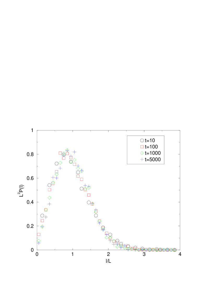
Figure 1: Plot of the scaling function $P_{sc}(x)$ against the scaled length $x$ from numerical simulations. Both the linear small-$x$ and gaussian large-$x$ behaviour are reproduced.

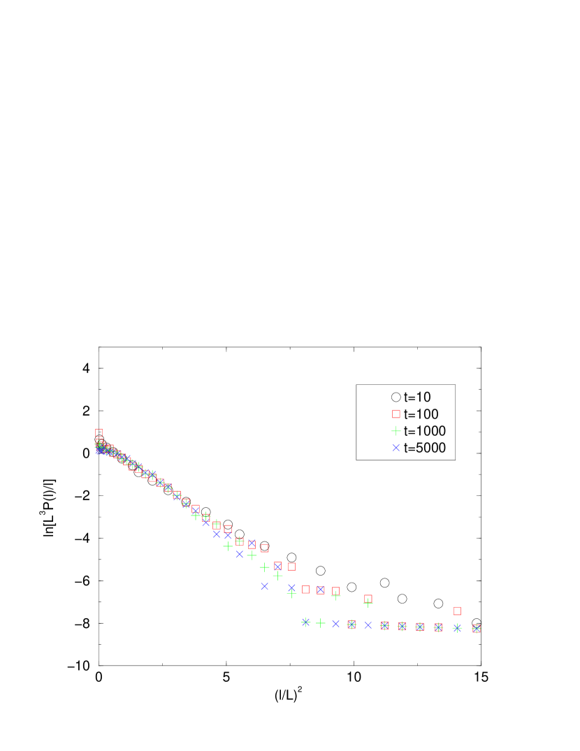
Figure 2: The data of Fig.1 plotted instead as $\ln(P_{sc}x^{-1})$ versus $x^{2}$

Returning to the rate of decay of N(t) we can write, in the general case,

$$\frac{dN}{dt} = -2\left(\left\langle l_{-}^{-1}\right\rangle\frac{\partial P_{+}(l_{+})}{\partial l_{+}}\mid_{l_{+}=0}\right.$$ (4)

$$+\left.\left\langle l_{+}^{-1}\right\rangle\frac{\partial P_{-}(l_{-})}{\partial l_{-}}\mid_{l_{-}=0}\right)$$

$$= -2\left(\left\langle l_{-}^{-1}\right\rangle\frac{\alpha_{+}}{L_{+}^{3}}+\left\langle l_{+}^{-1}\right\rangle\frac{\alpha_{-}}{L_{-}^{3}}\right)\ .$$

In the above expression we have used the fact that the rate for the elimination of $+$ and $-$ domains with $l=1$ is given by the mean rate at which $-$ and $+$ domains diffuse, i.e.  $\langle l_{-}^{-1}\rangle$ and $\langle l_{+}^{-1}\rangle$ respectively. The extra factor of 2 comes from the fact that the elimination of a domain reduces the number of domains by 2 (since the domains neighbouring the eliminated domains merge). For an exact result, these averages should be taken only over domains adjacent to domains of size $l=1$. In order to make further progress, we relax this condition and take the average over all domains of a given size. We are therefore neglecting correlations between domain sizes.

The required averages $\langle l_{\pm}^{-1}\rangle$ are given by

$$\langle l_{\pm}^{-1}\rangle=\frac{\int_{0}^{\infty}l_{\pm}^{-1}P_{\pm}(l_{\pm})dl_{\pm}}{\int_{0}^{\infty}P_{\pm}(l_{\pm})dl_{\pm}}={\Large\frac{2\alpha_{\mp}}{N(t)L_{\pm}^{2}}}f_{0}\ ,$$ (5)

where $f_{n}=\int_{0}^{\infty}x^{n}F(x)dx$ and $N(t)$ is the total number of domains per lattice site. The latter is obtained by adding the contributions $N_{+}(t)$ and $N_{-}(t)$ from $+$ and $-$ domains respectively:

$$N(t)=\int_{0}^{\infty}P_{+}(l{+})dl_{+}+\int_{0}^{\infty}P_{-}(l{-})dl_{-}=$$

$$=\left(\frac{\alpha_{+}}{L_{+}}+\frac{\alpha_{-}}{L_{-}}\right)f_{1}=\frac{2\alpha_{+}f_{1}}{L_{+}},$$ (6)

where the last equality follows from the condition $N_{+}(t)=N_{-}(t)$ for all $t$, and holds for all values of the conserved quantity $\mu$ defined as the fraction of spins which have the value $+1$ (i.e. the magnetisation per site is $2\mu-1$). This quantity satisfies

$$\mu=\int_{0}^{\infty}l_{+}P_{+}(l_{+})dl_{+}=\alpha_{+}f_{2}$$ (7)

and

$$1-\mu=\int_{0}^{\infty}l_{-}P_{-}(l_{-})dl_{-}=\alpha_{-}f_{2}.$$ (8)

Using Eqs. (5),(6), (7) and (8) we can express $\langle l_{\pm}^{-1}\rangle$, $L_{\pm}$ and $\alpha_{\pm}$ in terms of $N(t)$, $\mu$ and the integrals $f_{n}$ ($n=0,1,2$). Putting these into Eq.  (4) and integrating yields the following expression for the domain density :

$$N(t)=\left(\frac{3f_{0}f_{2}^{3}t}{8f_{1}^{5}\mu^{2}(1-\mu)^{2}}+\frac{1}{N(0)^{3}}\right)^{-1/3}\ .$$ (9)

It remains to determine the constants $f_{n}$. From the definition of the average domain lengths we find:

$$L_{\pm}=\frac{\int_{0}^{\infty}l_{\pm}P_{\pm}(l_{\pm})dl_{\pm}}{\int_{0}^{\infty}P_{\pm}(l_{\pm})dl_{\pm}}=\frac{f_{2}}{f_{1}}L_{\pm}$$

$$\Rightarrow f_{2}=f_{1}\ .$$ (10)

For the assumed Gaussian scaling function $F(x)=\exp(-\lambda x^{2})$, the required integrals give $f_{0}=(\pi/4\lambda)^{1/2}$, $f_{1}=1/(2\lambda)$ and $f_{2}=(\pi/16\lambda^{3})^{1/2}$. The result $f_{2}=f_{1}$ fixes $\lambda=\pi/4$, giving $f_{0}=1$ and $f_{1}=f_{2}=2/\pi$. The final expression for N(t) becomes:

$$N(t)=\left(\frac{3\pi^{2}t}{32\mu^{2}(1-\mu)^{2}}+\frac{1}{N(0)^{3}}\right)^{-1/3}\ .$$ (11)

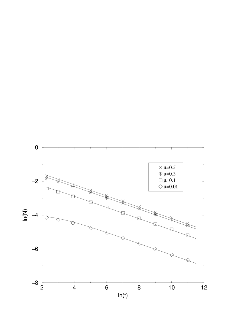
Figure 3: Time-dependence of the total domain density, $N(t)$, for different volume fractions, $\mu$, of the $+$ phase. The continuous curves show the analytical prediction given by Eqn. (reffinal).

In Figure 3 we have plotted eq.(11) for different values of $\mu$ together with numerical data from simulations described in the following subsection. The agreement is good even at early times, verifying the fast collapse to scaling observed in Figure 1. Note that in the derivation of Eq. (11) we used the scaling form (3) for all times $t$, not just late times. This may account for the small discrepancies between theory and data evident at early times in Figure 3. It is also evident that the data points lie slightly above the corresponding continuous curves at late times. Nevertheless, the generally good fit of Eq. (11) to the data, over a wide range of $\mu$ and with no adjustable parameters, provides good evidence that the assumptions made in its derivation are either correct or at least very good approximations. Principal among these assumptions are the Gaussian form taken for the scaling function $F(x)$ (to derive explicit expressions for $f_{0}$, $f_{1}$ and $f_{2}$), the assumption that this scaling function is the same for both domain types, and the neglect of correlations between domain sizes.

To probe the quality of the fit more closely, we extract the amplitude $C$ in the asymptotic behaviour $N(t)\to Ct^{-1/3}$ for large $t$. For $\mu=1/2$, we find $C=0.440\pm 0.003$, whereas the analytic form (11) gives $C=0.407$, a 7.5% discrepancy. Ben-Naim and Krapivsky krapivsky98 have given an alternative treatment of the domain-size distribution, making only the assumption that the domain sizes are uncorrelated. This leads to a slightly better value, 0.415, for $C$. However, no results were given for other values of $\mu$ in ref. krapivsky98 . Our data show that the calculated $C$ is smaller than the measured one by about 7.5% for $\mu=0.3$ and 0.1, and by about 5% for $\mu=0.01$.

II.2 Persistence probability

For the numerical simulations we adopted the domain description of the spin problem, since it is the most appropriate for $T\rightarrow 0$. We worked on 1D lattices of size $n=10^{5}$ with periodic boundary conditions. All samples were prepared by randomly assigning spins to the $n$ sites, although the system can be prepared in any other homogeneous initial state. The early-time form of the domain size-distribution is irrelevant to the asymptotic behaviour.

Updating the persistence probability $Q(t)$ means tracking the fraction of spins that have not flipped or, equivalently, the fraction of sites that have not been visited by a domain wall up to $t$. On average, we expect each of the $N$ domains to attempt to move by spin emission once per unit time in agreement with the rescaled rates, so a simple Monte-Carlo algorithm would be to select a domain at random, move it with probability $1/l$ in either direction, where $l$ is the its length, and increment time by $\Delta t=1/N(t)$ irrespective of whether or not the domain is moved. This is indeed the method used in sire98 to infer the value of the persistence exponent, $\theta=0.73$.

Unfortunately this algorithm suffers from severe slowing-down in the scaling limit, where the average domain length $L$ is much larger than unity and most hopping attempts are unsuccessful. We worked with a modified version of the domain algorithm which does not exhibit such problems by ensuring that a move is accepted at each computational step. A normalized vector is constructed for the $N$ domains, whose $i^{th}$ element, $H_{i}(t)=l_{i}^{-1}/(\sum_{i=1}^{N}l_{i}^{-1})$, is the probability that domain $i$ experiences a hop at time $t$. For any given hop this probability is size-dependent only. Incrementing time by $1/\sum_{i=1}^{N}l_{i}^{-1}$, the average time between successful moves, we end up with the same diffusion rate as in the simpler algorithm. We avoid, however, the problematic behaviour relating to the inefficiency of the $1/l$ trial. The disadvantage here is the calculation of the vector ${\bf H}$ at early times, which does result in the simpler algorithm being faster in this regime, but this is a small price to pay. We show in section III.3 that slow convergence to a scaling state in systems with diffusion rates $D\sim l^{\gamma}$ with $\gamma<-1$ reinforces the need for the new algorithm.

In Figure 4 we present a log-log plot of the persistence probability against time, averaged over 94 realisations. The effective exponent $\theta(t)=-d\ln Q/d\ln t$, plotted against $\ln t$ in the inset of Fig. refg-1, seems to saturate at value $\theta\simeq 0.716$, the spread around this value beyond $t\sim e^{11}$ being primarily due to poor statistics resulting from the small number of persistent sites remaining at this timescale.

We note that, since $\theta\approx 0.7$ is larger than the domain-growth exponent ($\phi=1/3$), the typical distance between persistent sites, $t^{\theta}$, grows faster than the domain length, $t^{\phi}$. Clusters of non-persistent sites, of typical length $t^{\theta}$, grow by the motion of the domain walls at their boundaries. These motions are uncorrelated since the separation, $t^{\theta}$, of the relevant walls is much larger than the domain scale. The statistical independence of persistence-destroying processes suggests further that the distribution function, $n(s)$, of the size $s$ of non-persistence intervals should decay exponentially, $n(s)\propto\exp(-s/\langle s\rangle)$, where $\langle s\rangle\sim t^{\theta}$ is the mean size of a non-persistent interval manoj00 . This is to be contrasted with the Glauber model, in which the persistence length, $t^{3/8}$, is smaller than the domain scale, $t^{1/2}$, and $n(s)$ has a nontrivial form manoj00 .

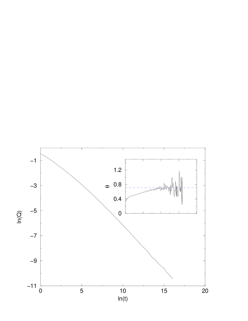
Figure 4: Logarithm of the persistence probability against $t^{\prime}=\ln t$. The local slope $\theta(t^{\prime})$ is also given in the inset.

III Conserved dynamics in aggregation

In this section we compare the coarsening dynamics of the Kawasaki model to that of aggregation models. How would the coarsening properties be modified in the Kawasaki ferromagnet for choices of the diffusion exponent $\gamma$ other than $\gamma=-1$ in $D\sim D_{0}l^{\gamma}$? Furthermore, is the amplitude ratio $R_{0}=D_{0}^{(+)}/D_{0}^{(-)}$ of the diffusion constants of the $+$ and $-$ domains relevant to the persistence probability and, if so, will a distinction between ‘up’ and ‘down’ persistence be necessary? We discuss these points with the aid of results from irreversible cluster-cluster aggregation and extensive numerical simulations of modified versions of the Kawasaki system. For the rest of the paper we shall use ‘Kawasaki’ to denote a more flexible model where we allow $\gamma\neq-1$ and $R_{0}\neq 1$. It must be pointed out, that both $D\sim 1/l$ and particularly $D_{0}^{(+)}=D_{0}^{(-)}$ are robust features of Kawasaki dynamics, which follow directly from the elementary spin processes. This follows most strongly from the symmetric nature of the emission process where both an ‘up’ and a ‘down’ spin are emitted during a single event and consequently $R_{0}=1$ is unavoidable. Although it is not possible to reconcile these rules with spin-exchange at the microscopic level, changes in the diffusion exponent and the ratio of amplitudes are easily accommodated in the domain description that we have employed so far.

III.1 Diffusion-limited cluster-cluster aggregation (DLCA)

Irreversible cluster aggregation is closely related to Kawasaki dynamics. It, too, involves the separation of a two-phase mixture through domain diffusion and leads to conservation of its respective order parameter, in this case the total mass $m$. Clusters, defined as intervals of consecutive occupied sites, move randomly and coalesce irreversibly on impact, whilst the ‘empty’ phase through which the clusters diffuse is immobile (reversible aggregation scenarios, including various fragmentation mechanisms or monomer ‘chipping’ majumdar , can actually result in effective diffusion of the empty phase, and hence partly restore the dynamic equivalence). Consequently, this model corresponds to the $R_{0}=0$ ‘Kawasaki’ system. The diffusion rate for a cluster of length $l$ is $D_{F}\sim l^{\gamma}$ but we shall concentrate on $\gamma\leq 0$ and particularly on $\gamma=0,-1$, which correspond to artificial but instructive realizations of domain diffusion on the Ising lattice.

Due to the broken mobility symmetry between the ‘filled’ (cluster) and ‘empty’ phases, a distinction should be made between the persistence properties of initially occupied sites and initially empty ones. Therefore, we use $P_{E}(t)$ to denote the persistence probability of empty sites and $P_{F}(t)$ that of occupied sites with similar notation applying to the corresponding exponents. Only $P_{E}$ is universal whereas $P_{F}$ depends strongly on the volume fraction $\mu$ of the ‘filled’ phase, which of course remains constant throughout the coarsening process.

Figure 5: Log-log plot of the domain density with time for $\gamma=-6$ to $-1$ (top to bottom). The asymptotic slopes are -0.117,-0.136,-0.162,-0.197,-0.248 and -0.332 respectively, in reasonable agreement with the prediction $\phi=1/(2-\gamma)$.

For negative $\gamma$ the exponents governing the algebraic decay of the cluster density and empty persistence probability have been calculated hellen01 to be $\phi^{cc}=1/(2-\gamma)$ and $\theta_{E}=2\phi^{cc}$ for the DLCA model. The dependence of the dynamic exponent on $\gamma$ is readily obtainable from scaling alone hellen00 , an approach whose validity extends to ‘Kawasaki’ dynamics in view of sec.II.1. If the domain scale is $l$, the time required to develop this scale is $t\sim l^{2}/D(l)\sim l^{2-\gamma}$, whence $l\sim t^{1/(2-\gamma)}$. For the empty-site persistence, i.e.  the probability that an initially empty site has not been covered by a cluster up to time $t$, Helen et al. used $D(t)=D_{0}t^{\gamma\phi}$ as a mean-field representation of the cluster kinetics to get $\theta_{E}$, which is known to be exact for $\gamma=0$. Numerical simulations indicate that the persistence of the ‘filled’ phase also decays algebraically with a non-universal exponent $\theta_{F}(\mu)$ and that $\theta_{F}=\theta_{E}$ in the half-filled case, $\mu=1/2$, for all $\gamma$.

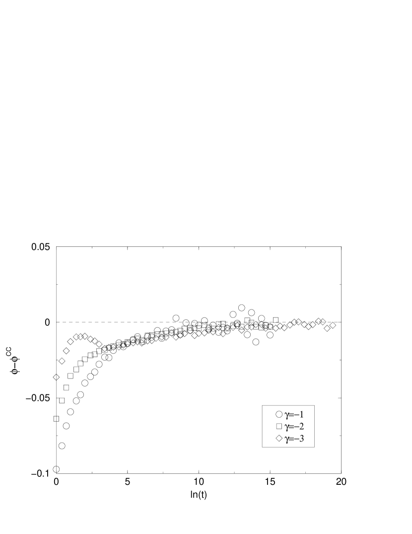
Figure 6: Plot of the difference $\phi-\phi^{cc}=\phi(R_{0}=1)-\phi(R_{0}=0)$ in logarithmic time, for 3 values of $\gamma$.

Agreement with simulations of the zero-magnetisation ‘Kawasaki’ model is very good for the form of the dynamic exponent in the regime $-1\leq\gamma\leq-6$ (Fig.5). The time required to reach the asymptotic value seems independent of the diffusion exponent $\gamma$ (Fig.6), so that all $\theta(\gamma)$ saturate within the numerical window. The data suggest that domain growth is identical for the limiting cases $R_{0}=0$ (aggregation) and $R_{0}=1$ (’Kawasaki’). We believe this to be the case in the whole range $0\leq R_{0}\leq 1$, given eq.(4) and simulations indicating no systematic change in $\phi(\gamma=0)$ for constant but unequal diffusion coefficients (Fig.7).

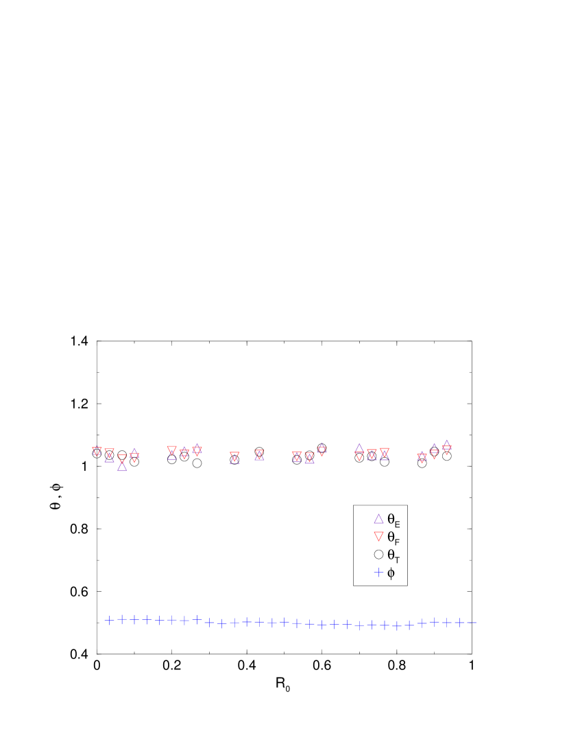
Figure 7: Dynamic and persistence exponents for the size-independent ‘Kawasaki’ model in the range $0\leq R_{0}\leq 1$. We have chosen $D_{E}=D_{+}$. The upper and lower data sets give the persistence and growth exponents, $\theta$ and $\phi$, respectively; $\theta_{T}$ refers to the persistence of the whole lattice and is obtained from the sum of the two constituent probabilities. The values of the exponents are consistent with $\phi^{cc}=1/2$ and $\theta^{cc}=1$.

III.2 The cases $\gamma=0,-1$

Let us examine size-independent diffusion ($\gamma=0$) first. The empty-site persistence probability for $R_{0}=0$ reduces to the survival probability of a stationary point surrounded by two random walkers – the near edges of the two domains surrounding the point (Fig.8(a)). This survival probability is given by the product of the survival probability due to each walker and therefore decays asymptotically as $t^{-1/2}t^{-1/2}=t^{-1}$. Similarly, we can interpret filled-site persistence as the survival probability of a random walker with receding boundaries (Fig.8(b)). The persistent site carries the diffusion of the domain in which it lies, while the edges expand away from it due to domain collisions. For any other $R_{0}$ the survival of the persistent site involves a mixture of both processes (Fig.8(c)).

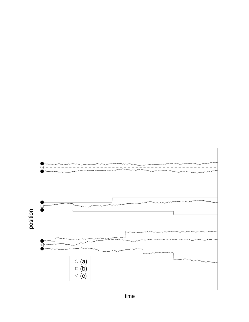
Figure 8: Space-time diagram of persistence-destroying processes in (bottom to top) (a) empty, (b) filled and (c) symmetric phases.

Although the exact kinetics of individual walls in Fig.8(c) remain unknown, hints as to their form have emerged in many contexts. In a study of annihilating random walks on the infinite half-line krapivsky97 it was shown from numerical measurements that the probability density of the outermost particle is asymmetric. In that case too the trajectory of the outermost walker is a combination of diffusion and directed jumps resulting from particle annihilation, similarly to Kawasaki walls. The probability density curve was found to decay like $\exp{(-\alpha x^{2})}$ in the direction of the free interface, but like $\exp{(-\beta x)}$ on the side of the filled lattice, a behaviour which seems to suggest a regime where the diffusion exponential dominates and one where the annihilation exponential does. This appears reasonable on the basis that the contribution of these irregular hops is super-diffusive, characterised by the domain length distribution from which the jumps are drawn. In studies of the $A+A\rightarrow 0$ reaction, this component has indeed been shown to exhibit an exponential form of the kind $\exp{(-\beta x)}$derrida96 . Unfortunately, our calculation on a naive convolution of the two components has turned out an overestimate of the persistence exponent in the case where the persistent site is stationary and the probability can be expressed as the product of the two individual capture probabilities, suggesting that correlations between the diffusion and annihilation processes cannot be neglected.

As far as numerical simulations of the size-independent system are concerned, we have found that within the accuracy of the statistics, no systematic shift in the values of the exponents takes place in the transition from irreversible aggregation to symmetric diffusion. It should be noted that the data in Fig.7 consistently fall slightly above the predicted value $\theta=1$. Since the exponent is known to be 1 in the limiting cases $R_{0}=1$ and $R_{0}=0$ hellen01 it may be that the numerics have not yet reached the true asymptotic value. Nevertheless, even considering this small discrepancy along all values of $R_{0}$, $\gamma=0$ remains the only case for which the values of all four exponents match in the limits $R_{0}=0$ and $R_{0}=1$. For Kawasaki dynamics ($\gamma=-1$), which we discussed in Sec.II.2, a deviation of $\theta$ from $\theta_{cc}$ is visible and begins to grow as we reduce the diffusion exponent further (see, Sec.III.3). The inset in Figure 4 indicates that $\theta$ saturates asymptotically above the $2/3$ aggregation value, our calculations favouring $\theta=0.716(5)$.

III.3 $-2\geq\gamma\geq-6$

In this parameter range, the aggregation and ‘Kawasaki’ results for the persistence exponent clearly disagree. Our simulations did not reach, in most cases, the asymptotic regime (Fig.9). Nevertheless, they demonstrate that the exponents invariably exceed the aggregation prediction $\theta_{cc}=2/(2-\gamma)$. The very slow convergence we observe has, in fact, also arisen in other studies of aggregation-fragmentation models rajesh02 , a class to which the ‘Kawasaki’ model can be shown to relate. It was noted there, in numerical estimates of the cluster mass distribution function, that for $\gamma<-2$ simulations failed to approach a scaling state in the time available. Our own efforts led us in many cases to final configurations where the average domain size was comparable to the lattice size. We think that for the algorithm employed, good scaling-state statistics would require unfeasibly long runs. We found no obvious way in which to improve further the performance of the routine which is still limited by the update of the probability vector $H$, although this penalty becomes less relevant at late times. Unfortunately, lattice renormalisation techniques (such as the one in ben-avraham ) which have proven successful in other circumstances can not be used in this case as they lead to local violations of the conservation principle.

It is also clear that the collapse onto a single curve encountered in Figure 6 at large $t$ is absent for the persistence exponent. This much slower approach to asymptotic behaviour for $\theta$ than for $\phi$ is also consistent with the statement made in Sec.II.2 that non-persistent intervals and domain lengths have different scaling characteristics.

Figure 9: Effective persistence exponent against $\ln t$ for $R_{0}=1$ ‘Kawasaki’ systems with negative $\gamma$. The horizontal lines mark the values $\theta^{cc}$ predicted for $R_{0}=0$.

Despite these complications, lower limits for $\theta(\gamma)$ are set by the data, and imply faster-than-$\theta^{cc}$ decay for $Q$ in the symmetric system. This is perhaps surprising in view of the results in the previous subsection, where such a deviation from the $R_{0}=0$ behaviour is absent. We do not know of any argument for the $\gamma=0$ system to constitute a special case, but it is tempting to conjecture that the deviation of $\theta$ from $\theta^{cc}$ observed for all $\gamma<-1$ is monotonic in the intermediate regime $0<R_{0}<1$.

IV Discussion and Summary

In this paper we considered an integrated analysis of two-phase conserved systems in one dimension based on two examples: irreversible cluster-cluster aggregation, where only one of the phases is allowed to diffuse, and Kawasaki dynamics, where both phases diffuse at the same rate. In terms of the ratio of diffusion amplitudes $R_{0}$, the algebraic domain growth at late times has been established as identical in the these two limits, with the ‘Kawasaki’ dynamic exponent $\phi$ matching the prediction $1/(2-\gamma)$ whatever the form of size-dependence assumed for the diffusion rate. In the case of size-independent diffusion, we have also found that this equivalence holds for all other intermediate values of $R_{0}$, as was expected given the restrictions on scaling imposed by the conservation principle, i.e.  that the order parameter should remain constant throughout coarsening. The robustness of this behaviour has been confirmed in a variety of aggregation systems rajesh02 ; hellen01 .

By contrast, in the critical $\mu=1/2$ limit considered, changes in the relative mobility of the two phases lead to different persistence characteristics. The transition from irreversible aggregation to symmetric diffusion is accompanied by severe slowing-down in the convergence rate of the effective persistence exponent to its asymptotic value as well as a distinct shift from the simple $\theta^{cc}=2/(2-\gamma)$ result for all negative $\gamma$. We have been able to show that the disagreement, which is at zero $\gamma$ absent in the whole range $0\leq R_{0}\leq 1$, always leads to faster persistence decay for the symmetric system, with numerical data indicating a possible lower bound for the exponent at $\theta=2.3\phi$ $(\gamma<-2)$.

Apart from the slow convergence to asymptotic behaviour which hinders any definitive results as far as the value of $\theta$ in the symmetric limit is concerned, it is also possible that, for size-dependent cluster dynamics and finite values of $R_{0}$, $Q(t)$ deviates from the simple power-law behaviour observed in irreversible aggregation. In this latter case, it seems that the filled persistence (the persistence of the mobile phase) is non-universal and decays as a power-law only for $\mu=1/2$ hellen01 . Since single-site persistence for $R_{0}>0$ involves a mixture of both the empty- and filled-site behaviour, it is possible that the resulting probability is also non-universal.

A further prospect which must be considered is the possibility of inferring $\theta$ in the more strongly size-dependent systems from the scaling properties of the size-distribution of non-persistent sites. The general characteristics of this scaling are dictated by the fact that $\theta>\phi$, which constrains the tail of the non-persistent interval size-distribution to a known form manoj00 . Hints of this behaviour have been suggested by our results for the probability $Q(t)$, since the regularity encountered in the collapse of the growth exponent onto the aggregation result for different $\gamma$ is lost in plots of $\theta$. Instead, a very slow saturation of the local persistence exponent has been observed extending, in all cases but $\gamma=-1$, well beyond $t\sim e^{15}$.

V ACKNOWLEDGEMENT

The work of PG was supported by EPSRC.

References

- (1) A. J. Bray, Adv. Phys. 43, 357 (1994).
- (2) B. Derrida, A. J. Bray, C. Godreche, J. Phys. A 27, 357 (1994).
- (3) B. Derrida, V. Hakim, V. Pasquier, Phys. Rev. Lett. 75, 751 (1995).
- (4) S. N. Majumdar, Curr. Sci. India 77, 370 (1999), and cond-mat/9907407.
- (5) S. J. Cornell, A. J. Bray, Phys. Rev. E 54, 1153 (1996).
- (6) D. ben-Avraham, F. Leyvraz, S. Redner, Phys. Rev. E 50, 1843 (1994).
- (7) S. Cueille, C. Sire, Eur. Phys. J. B 7, 111 (1999).
- (8) E. K. O. Hellen, M. J. Alava, Phys. Rev. E 66, 26120 (2001).
- (9) S. J. Cornell, K. Kaski, R. B. Stinchcombe, Phys. Rev. B 44, 12263 (1991).
- (10) E. Ben-Naim, P. L. Krapivsky, J. Stat. Phys. 93, 583 (1998).
- (11) C. Jepessen, O. G. Mouritsen, Phys. Rev. B 47, 14724 (1993).
- (12) E. K. O. Hellen, T. P. Simula, M. J. Alava, Phys. Rev. E 62, 4752 (2000).
- (13) R. Rajesh, D. Das, B. Chakraborty, M. Barma, Phys. Rev. E 66, 56104 (2002).
- (14) G. DeSmedt, C. Godreche, J. M. Luck, Eur. Phys. J. B 27, 363 (2002).
- (15) G. Manoj, P. Ray, J. Phys. A 33, 5489 (2000); S. J. O’Donoghue and A. J. Bray, Phys. Rev. E, 62, 3366 (2000).
- (16) L. Frachebourg, P. L. Krapivsky, S. Redner, J. Phys. A 31, 2791 (1998).
- (17) B. Derrida, R. Zeitak, Phys. Rev. E 54, 2513 (1996).
- (18) D. ben-Avraham, J. Chem. Phys. 88, 941 (1988).