[

Effects of interaction on an adiabatic quantum electron pump

Abstract

We study the effects of inter-electron interactions on the charge pumped through an adiabatic quantum electron pump. The pumping is through a system of barriers, whose heights are deformed adiabatically. (Weak) interaction effects are introduced through a renormalisation group flow of the scattering matrices and the pumped charge is shown to always approach a quantised value at low temperatures or long length scales. The maximum value of the pumped charge is set by the number of barriers and is given by $Q_{\rm max}=n_{b}-1$. The correlation between the transmission and the charge pumped is studied by seeing how much of the transmission is enclosed by the pumping contour. The (integer) value of the pumped charge at low temperatures is determined by the number of transmission maxima enclosed by the pumping contour. The dissipation at finite temperatures leading to the non-quantised values of the pumped charge scales as a power law with the temperature ($Q-Q_{\rm int}\propto T^{2\alpha}$), or with the system size ($Q-Q_{\rm int}\propto L_{s}^{-2\alpha}$), where $\alpha$ is a measure of the interactions and vanishes at $T=0~{}(L_{s}=\infty)$. For a double barrier system, our result agrees with the quantisation of pumped charge seen in Luttinger liquids.

]

In the last few years, there has been a lot of interest in the phenomenon of electron transport at zero bias via the mechanism of adiabatic pumping. The parameters of a system are slowly varied as a function of time, such that they return to themselves after each cycle, and the net result is charge transport[2]. The idea of quantised charge pumping was first introduced by Thouless[3] for a spatially periodic system, where the quantisation could be proved using topological arguments. This was further investigated theoretically in Refs.[4].

Experimentally, the possibility of transferring an integer number of charges through an unbiased system has been achieved in small semi-conductor dots in the Coulomb blockade (CB) regime[5, 6]. It has also been achieved in surface-acoustic-wave based devices[7], but here too, the quantisation has been attributed to CB. An adiabatic electron pump that produces a dc voltage, in response to a cyclic change in the confining potential of an open quantum dot has also been experimentally constructed[8]; however, here the charge is not quantised.

The open dot quantum pumps, where the quantum interference of the wave-function, rather than the Coulomb blockade, plays a dominant role, has been of recent theoretical interest. A scattering approach to such a pump was pioneered by Brouwer[9] and others [10, 11], who, building on earlier results[12], related the pumped current to derivatives of the the scattering matrix. Using this approach, there have been several recent theoretical studies [13, 14, 15, 16, 17, 18, 19, 20, 21, 22, 23, 24, 25, 26, 27, 28, 29, 30, 31, 32]. The conditions under which the charge is (almost) quantised in open quantum dots, has been explored in detail in Refs.[33, 34, 35, 36]. Ref.[33] shows that the pumped charge is produced by both nondissipative and dissipative currents. It also shows that charge quantisation is achieved when the dissipative conductance vanishes. This is also emphasized in Ref.[36], where the adiabatic charge transport in a Luttinger liquid has been studied. In Refs[34, 35], the correlation between the conditions for resonant transmission and quantised charge has been emphasized.

In this paper, we include the effects of inter-electron interactions along with the interference effects, using a renormalisation group (RG) method developed recently[37, 38, 39, 40] for the flow of the scattering matrices. We show that at low temperatures, the inclusion of interactions, leads to quantisation of the pumped charge. As seen earlier in Refs.[33] and [36], we find that the charge pumped is a sum of two terms - a quantised term, and a dissipative term. The quantised term, which is topological in nature and is due to quantum interference is always present. For non-interacting electrons, the dissipative term is also large and masks the quantisation due to the first term. However, the RG flow of the $S$-matrices, due to the interaction, causes the dissipative term to vanish at long length scales or low temperatures making the quantisation of the pumped charge visible.

FIG. 1.: Schematic diagram of a multiple dot system ($n_{d}$ dots or $n_{b}+1$ barriers) defined on a two dimensional electron gas. The barriers forming the dots are denoted as $V_{b}$ and the gate voltages controlling the density in the dots are denoted as $V_{G}$.

The quantum pump is formed by a system of coupled quantum dots (shown in Fig.1), where the barriers forming the dot are periodically modulated as

$$V_{i} \equiv V_{1}=V_{0}+V_{p}\cos(\omega t),~{}i\leq n_{b}/2~{}{\rm for}~{}n_{b}={\rm even},$$ (2)

$$\quad i\leq n_{b}/2+1~{}{\rm for}~{}n_{b}={\rm odd},$$

$$V_{i} \equiv V_{2}=V_{0}+V_{p}\cos(\omega t+\delta),~{}{\rm for~{}the~{}remaining}.$$ (3)

Clearly, for $n_{b}$ barriers, we have $n_{d}=n_{b}-1$ dots. Here $\omega$ is related to the time period as $\omega=\tau/2\pi$ and $\delta$ is the phase difference between the two time-varying potentials. Since this potential breaks the parity symmetry, it allows the shape of all the dots to be varied. As has been emphasized earlier, this is a necessary condition to get non-zero pumped charge.

Although we use $\delta$-function barriers, we expect the calculations to be robust to changing the form of the barriers. Following the work of Ref.[41], we also expect these results to be robust to weak disorder. We treat the dot within a one-dimensional effective Hamiltonian[42], since they are coupled to the leads by a single channel quantum point contact. (Although in real quantum dots, transmission properties can fluctuate and energy level spacings can vary and can even be chaotic, this modelling works to understand simple physical features of higher dimensional quantum dots.) The width of the dots (effectively the width of the quantum well that we use) is given by $a$. We are mainly interested in the region where $V_{0}\leq E_{F}$ since we wish to study the resonant tunneling regime and not the CB regime.

The effective two-channel $S$-matrix for this system of $n_{b}$ barriers can be written as

$$S=\left(\begin{array}[]{ll}re^{i\theta}&fe^{i\phi}\\ fe^{i\phi}&re^{i\theta^{\prime}}\end{array}\right)$$ (4)

where the parameters $r,f,\theta,\theta^{\prime}$ and $\phi$ are functions of the Fermi energy $E_{F}$ and the amplitudes of the time- varying potentials $V_{i}(t)$. Their explicit forms can be found, in terms of the parameters of a single well, (in the adiabatic limit), by solving the time-independent Schrodinger equation for the potential $V_{i}(t)$ given in Eq. 3, for each value of $t$. The reflection coefficients are not the same (phase can differ) because the time-varying potentials explicitly violate parity. The potential also violates time-reversal invariance. But since in the adiabatic approximation, we are only interested in snapshots, at each value of the time, the Hamiltonian is time-reversal invariant and hence, the transmission amplitudes are the same for the ‘12’ and ‘21’ elements in the $S$-matrix.

By the Brouwer formula[9], the charge pumped can directly be computed from the parametric derivatives of the $S$-matrix. For a single channel, it is given by

$$Q = {e\over 2\pi}\int_{0}^{\tau}dtIm{(}{\partial S_{11}\over\partial V_{1}}S_{11}^{*}{\dot{V}_{1}}+{\partial S_{12}\over\partial V_{1}}S_{12}^{*}{\dot{V}_{1}}$$ (6)

$$~{}~{}~{}~{}~{}~{}~{}~{}~{}~{}\quad+{\partial S_{11}\over\partial V_{2}}S_{11}^{*}{\dot{V}_{2}}+{\partial S_{12}\over\partial V_{2}}S_{12}^{*}{\dot{V}_{2}}{)}$$

where $S_{ij}$ denote the matrix elements of the $S$-matrix and ${\dot{V}_{1}}$ and ${\dot{V}_{2}}$ are the time derivatives of the $V_{1},V_{2}$ given in Eq. 3. Thus, the pumped charge is directly related to the amplitudes and phases that appear in the scattering matrix. For the form of the $S$-matrix given in Eq. 4, this is just

$$Q={e\over 2\pi}\int_{0}^{\tau}[{\dot{\theta}}-f^{2}({\dot{\theta}}-{\dot{\phi}})]dt$$ (7)

where the first term is clearly quantised since $e^{i\theta}$ has to return to itself at the end of the period. So the only possible change in $\theta$ in a period can be in integral multiples of $2\pi$ -i.e., $\theta(\tau)\longrightarrow\theta(0)+2\pi n$. The second term is the ‘dissipative’ term which prevents the perfect quantisation. It is easy to see the analogy of Eq. 7 with Eq. 19 of Ref.[33].

The correlation between resonant transmission and the pumped charge has been studied earlier by several groups[17, 27, 31, 34, 35]. A pumping contour[34, 35] can be defined in the plane of the parameters, $V_{1}$ and $V_{2}$, as the closed curve traced out in one cycle of modulation of the barriers ($t\rightarrow t+\tau$). As we shall see below explicitly, the value of the first term in Eq. 7 is set by the number of transmission maxima enclosed by the pumping contour, whereas the second term depends on how peaked the transmission function is, around its maxima. We find that the more peaked the transmission function, the smaller is the dissipation.

The aim of this paper is to study the effect of electron-electron interactions on the charge pumped. In Ref.[36], a bosonised approach was used; here, the barriers have to be either in the weak back-scattering or the strong back-scattering limit. But for time-dependent potentials, within a single pumping cycle, the barriers can range from the weak barrier to strong barrier limits, if the perturbing potential is large. Contours with such large perturbing potentials are required for enclosing multiple transmission maxima, which, in turn, lead to larger pumped charges. Hence, it is much more convenient to introduce interactions (provided they are weak) perturbatively and directly obtain the renormalisation group (RG) equations for the entries of the $S$-matrix. This method has been used extensively in Refs.[38, 40] and we directly present the RG equations for the effective two-channel $S$-matrix given in Eq. 4 as follows -

$$\frac{dS}{dl}~{}=~{}M~{}-~{}SM^{\dagger}S~{}.$$ (8)

Here $M$ is a diagonal $2\times 2$ matrix given by

$$M=\left(\begin{array}[]{ll}{1\over 2}\alpha_{1}r&0\\ 0&{1\over 2}\alpha_{2}r\end{array}\right)~{}$$ (9)

and $l$ is the length scale. The dimensionless constants $\alpha_{i}$ are small and positive and are related to the Fourier transform of the short-range density-density interaction potential $V_{i}(x)$ in the two channels as

$$\alpha_{i}=\frac{({\tilde{V}}_{i}(0)-{\tilde{V}}_{i}(2k_{F})}{2\pi\hbar v_{F}}~{},$$ (10)

where we assume that the Fermi velocity is $v_{F}=\hbar k_{F}/m$. Thus, $\alpha_{i}$ is a measure of the inter-electron interactions. It can also be related to the bosonisation parameter $K$ as

$$K_{i}~{}=~{}\bigl{(}\frac{1-\alpha_{i}}{1+\alpha_{i}}\bigr{)}^{1/2}~{}.$$ (11)

When the barriers are symmetric (i.e., at some point in the pumping cycle when $V_{1}=V_{2})$), parity is not violated and we can set $\theta=\theta^{\prime}$ in Eq. 4. We will always run the RG equations at this point. For the computation of the pumped charge, the origin in $t$ is not relevant. We only need to compute the charge pumped in one cycle. It is also natural to expect the two channels to have the same inter-electron interactions; hence $\alpha_{i}=\alpha$. In that case, we obtain the following explicit equations for the RG flow of the transmission (and reflection) amplitudes and phases. We find

$${df\over dl} = -\alpha f(1-f^{2})~{},$$ (12)

$${d\phi\over dl} = 0~{},$$ (13)

for the flow of the transmission amplitude and phase and

$${dr\over dl} = {\alpha\over 2}r(1-r^{2}-f^{2}\cos 2(\phi-\theta))~{},$$ (14)

$${d\theta\over dl} = {\alpha\over 2}f^{2}\sin 2(\phi-\theta)~{},$$ (15)

for the flow of the reflection amplitude and phase. (Note that when $\theta\neq\theta^{\prime}$, two similar sets of equations can be obtained, both for $\theta$ and for $\theta^{\prime}$ using $S_{12}$ and $S_{11}$ for one and $S_{22}$ and $S_{21}$ for the other.) However, the condition of unitarity on the $S$-matrix in Eq. 4 implies that $\phi-\theta=\pi/2+2n\pi$. This simplifies the RG flow equations for the reflection amplitude and phase, so that they become similar to those for the transmission amplitude and phase, i.e.,

$${dr\over dl} = \alpha r(1-r^{2})~{},$$ (16)

$${d\theta\over dl} = 0~{}.$$ (17)

The entries of $S$ therefore become functions of the length scale $l$ or equivalently of $L$, where $l={\rm ln}(L/d)$, and $d$ is the short-distance cutoff which we take to be the average interparticle spacing. The RG flow can also be considered as a flow in the temperature since the length scale $L$ can be converted to a temperature $T$ using

$$L_{T}~{}=~{}\frac{\hbar v_{F}}{k_{B}T}~{},$$ (18)

as the thermal length. The interpretation of $L_{T}$ is that it is the thermal length beyond which the phase of an electron wave-packet is uncorrelated. Thus $L_{T}$ is the thermal phase coherence length. Hence, the RG flow has to be cutoff by either $L_{T}$ or the system size $L_{s}$, whichever is smaller[40]. In all our numerical computations, we start the RG flow at the microscopic length scale $d$, which is taken to be the inter-particle separation. We then renormalise to larger and larger length scales, stopping at either $L_{T}$ or $L_{s}$, whichever is smaller. Note that for a length $L=100\mu m$, the equivalent temperature as computed from Eq. 18 is $T=6.5mK$ (for $v_{F}=3\times 10^{7}cm/sec$, which is the typical value of the Fermi velocity in $GaAs$). Both of these are experimentally achievable. Hence, whether $L_{s}$ or $L_{T}$ is reached first depends on the given system. If $L_{T}>L_{s}$, we can continue the RG flow until we reach $L_{T}$, where phase coherence is lost due to thermal fluctuations.

In the rest of the paper, we compute the transmissions, the phases and the quantised charges as a function of the various parameters in the theory. We then show how the elements of the $S$-matrix, and consequently, the transmissions, the phases and the pumped charge change as a function of the RG flow. Since the RG flow is also a flow in temperature, we show how the pumped charge changes as we decrease the temperature and reaches quantised values at very low temperatures. However, note that the RG flow is cutoff by the physical size of the system at a temperature $T_{L_{s}}={\hbar v_{F}}/{k_{B}L_{s}}$ and one cannot go to lower temperatures. However, one can still continue the RG flow upto the length scale $L_{T}$, until the system loses thermal phase coherence. ( For illustrative purposes, though, we sometimes take the limit that the system size goes to infinity. In that case, the temperature can be lowered to $T=0$.) We will see that as we change the temperature, the pumped charge shows power law behaviour as a function of the temperature until we reach the system size. Beyond that, the pumped charge shows power law behaviour as a function of the system size. In the next few subsections, we explicitly study the double barrier system $n_{b}=2$, the triple barrier system $n_{b}=3$ and the quadruple barrier system $n_{b}=4$. We then extrapolate the results to an arbitrary number of barriers.

Strictly speaking, to remain within adiabatic approximation under which the Brouwer formula is derived, the energy level spacing in the dots $\Delta$ has to be larger than the energy scale defined by the frequency of the time-varying parameter $E_{\omega}=\hbar\omega$. It is only under this approximation that the snapshot picture of studying the static $S$-matrix for different time points within the period is valid. A better approach to go beyond the adiabatic approximation[25, 43] is to use the Floquet states. Here we remain within the adiabatic approximation even though $E_{F}\geq V_{0}$, by choosing the spacing between the barriers $a$ to be sufficiently small, so that the separation of the resonance level peaks ($\Delta>\hbar\omega$).

$\bullet$ Single dot case or $n_{b}=2$ :

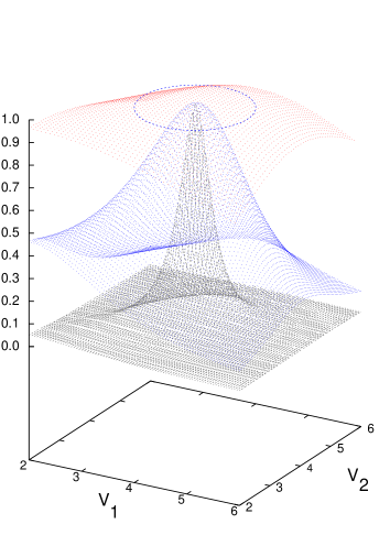
FIG. 2.: Transmission $F=f^{2}$ as a function of the barrier strengths $V_{1}$ and $V_{2}$ for three different values of $L=1,100,1000$ ($T_{L}=18K,0.18K,18mK$) for the double barrier system. For $V_{0}=4.0,V_{p}=1.0$, the pumping contour is shown as a dashed line. The other parameters are given by $E_{F}=8.4,\alpha=0.3,\omega=1$, $a=4$ and $\delta=\pi/2$. The pumped charges are $0.027,0.29,0.62$ for the three values of $L$ respectively.

Here, we compute the scattering matrix for two $\delta$-function barriers at a distance $a$ apart. To facilitate the generalisation to a larger number of barriers, we first obtain the $M$-matrix linking the incident wave to the left of a $\delta$-function barrier at $x=a$ to the transmitted wave to the right of the barrier, in terms of the strength $V$ of the potential, the distance $a$ and the energy of the incident wave $E_{F}$ as[31]

$$M=\left(\begin{array}[]{ll}1+{iV\over 2\sqrt{E_{F}}}&~{}~{}{iV\over 2\sqrt{E_{F}}}e^{-2ia\sqrt{E_{F}}}\\ -{iV\over 2\sqrt{E_{F}}}e^{2ia\sqrt{E_{F}}}&~{}~{}1-{iV\over 2\sqrt{E_{F}}}\end{array}\right)~{}.$$ (19)

The $S$-matrix which relates the outgoing waves to the incoming waves is simply obtained by rewriting the above matrix elements as

$$S=\left(\begin{array}[]{ll}M_{21}/M_{11}{}&~{}~{}~{}~{}~{}~{}1/M_{11}\\ ~{}~{}1/M_{11}{}&~{}-M_{12}/M_{11}\end{array}\right)~{}.$$ (20)

Since for a series of potential barriers, the transmitted wave can be simply obtained by multiplying the $M$-matrices, it is now easy to obtain the $S$-matrix for any number of barriers and thus identify the parameters $r,f,\theta,\theta^{\prime}$ and $\phi$ in terms of the parameters of the potential scattering such as the distance $a$, the potential strengths $V_{i}$ and the Fermi energy $E_{F}$. For two barriers, we find the elements of the $S$-matrix as

$$S=\left(\begin{array}[]{ll}Ae^{2ia\sqrt{E_{F}}}/B&~{}~{}~{}~{}1/B\\ ~{}~{}~{}1/B&Ae^{-2ia\sqrt{E_{F}}}/B\end{array}\right)~{},$$ (21)

where $A=-i(V_{1}+V_{2}e^{2ia\sqrt{E_{F}}})/2\sqrt{E_{F}}-V_{1}V_{2}(e^{2ia\sqrt{E_{F}}}-1)/4E_{F}$ and $B=1+i(V_{1}+V_{2})/2\sqrt{E_{F}}+V_{1}V_{2}(e^{2ia\sqrt{E_{F}}}-1)/4E_{F}$ and $V_{1}$ and $V_{2}$ are the strengths of the two barriers.

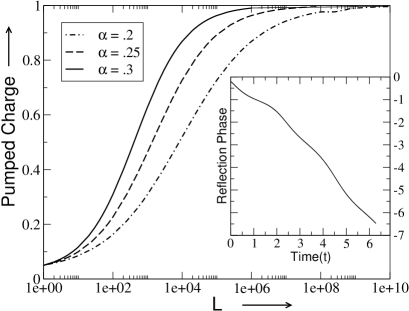
FIG. 3.: $Q$ (in units of $e$) as a function of the RG length scale, $L$ for three different values of the interaction strength $\alpha=0.2,0.25,0.3$ for the double barrier system. The values of the other relevant parameters are the same as in Fig. 2. The inset shows the change in the reflection phase in one pumping cycle to be 2$\pi$.

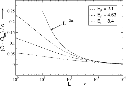
FIG. 4.: Scaling of the dissipative term $Q-Q_{\rm int}$ as a function of the length scale for the double barrier system. As seen in Eq. 24, for long length scales, the term that appears in the denominator can be ignored and the dissipation terms for different values of $E_{F}$ fall on the scaling curve $L^{-2\alpha}$ shown in the figure as a solid line. The contour chosen has $V_{0}=4.5$, $V_{p}=4.0$ and $\delta=\pi/4$.

Following Ref.[17], to obtain numerical results, we set the width of the well $a=4$ (in units of the inter-particle separation $a_{I}=100A^{o}$) and $\omega=1$. We find, as expected in the adiabatic approximation, that our results are independent of $\omega$ and hence $\omega$ can be made as small as we wish. We note that our results are periodic in $a$ for a fixed $E_{F}$ (see Eq.19) and hence the width of the well can be increased. However, to remain within the adiabatic approximation, $a$ is restricted by $\Delta>\hbar\omega$. Also, for any value of $a$, one can find the maximum for the pumped charge by tuning $E_{F}$[17, 31]. Our energy units are set by $\hbar=2m=k_{B}=1$, where $k_{B}$ is the Boltzmann constant. So for $GaAs$, with a typical inter-particle spacing $a_{I}=100A^{o}$, and a typical effective mass $m=0.07m_{e}$, if we wish to set $a_{I}=1$, the energy unit is $E=5.6meV$, (using $E=\hbar^{2}/2ma_{I}^{2}$) which corresponds to a temperature of $T=65^{o}K$ (using $E=k_{B}T$). The pumped charge for the double barrier system was obtained earlier in Refs.[17, 31] and shown to be very small. Here, we shall see that the reason for this is that the transmission is not peaked about the transmission maxima; in fact, it is rather flat. Hence, there is a large dissipative term in the pumped charge. We shall also see how interactions make the transmission more peaked about the maxima, reduces the dissipation and enhances the possibility of quantisation. We compute the transmission as a function of the barrier heights $V_{1}$ and $V_{2}$ and plot it in Fig. 2, for a range of $V_{i}$ between 2.0 and 6.0. The pumping contour[15] is defined as the closed path formed in the parameter space by the variation of the parameters in one cycle. Here, the varying parameters are $V_{1}$ and $V_{2}$. For this graphs, we choose the mean barrier height to be $V_{0}=4.0$ and the perturbation to be $V_{p}=1.0$. We also choose $\delta=\pi/2$ to maximise the pumped charge. (For the triple barrier and quadruple barrier cases, different pumping contours are chosen depending on what we need to illustrate). These parameters, using Eq. 3, define the pumping contour, shown in the $V_{1}-V_{2}$ plane in Fig. 2 as a dashed line. The top surface in Fig. 2 denotes the transmission (at the Fermi energy $E_{F}=8.4$, which is much above the barrier heights $4.0\pm 1.0$), without any renormalisation of the barriers due to interactions. It is essentially flat and only a small part of the region of high transmission is enclosed by the pumping contour. Thus, although the pumping contour encloses the transmission maximum, which essentially implies that the first term in Eq. 7 is unity, (see inset in Fig. 3, which shows that the reflection phase change in one pumping cycle is $2\pi$), the second dissipative term is very large and the pumped charge is vanishingly small ($Q=0.027$).

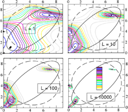
FIG. 5.: Contour plots of the transmission as a function of $V_{1}$ and $V_{2}$ for four different lengths $L=1,10,100,10,000$ for the triple barrier system. The maxima are shown in black and the separation between the contours is 0.05, whereas the white regions correspond to transmission less than 0.05. The colour coding for the transmissions starting from $F=1$ in black to $F=0.05$ in light gray, is shown in the last panel. The two pumping contours are for $V_{0}=4.5$, $V_{p}=4.0$ and $\delta=\pi/2$ for the dashed contour and $\delta=\pi/4$ for the solid contour. The pumped charges for each of the contours in each of the panels is given in the text. The other parameters are as given in Fig.(2).

We now use the RG equations in Eqs.12-17. Since the phases do not change under the RG flow, we only need to use Eq. 12, to compute the change in the transmission as a function of the length scale. We start the RG flow at $L=1=d=4\times 100A^{o}$, ($a=4$), which is the width of the well, and then renormalise to longer length scales, until we reach the size of the sample, which is at best $100\mu m$. At this length scale, the entire sample is phase coherent. In terms of temperature, the renormalisation is from $T=18K$ to $T=6.5mK$, which is well within the range of experimental feasibility. ( However, in many graphs, we show a much larger range of the renormalisation, assuming that the samples can be made phase coherent, over much longer length scales, simply for illustrative purposes.) We find that as the RG flow proceeds, the transmission maxima get more and more peaked as seen in Fig. 2, where we have plotted the transmissions at different points along the RG flow. The intermediate surface is when the length scale is $L=100$ or equivalently $T=.18K$. Here, the surface is clearly more peaked than the original surface and the pumpiong contour encloses a reasonable fraction of the non-zero transmission. The pumped charge turn out to be 0.29. The bottom surface is much more highly peaked and is the transmission at the length scale $L=1000$ or at $T_{L}=18mK$. Here, clearly, almost all the non-zero transmission is enclosed by the pumping contour and the pumped charge is 0.62. This narrowing of the transmission peaks is expected from Luttinger liquid studies of the double barrier[44], and this narrowing is what is responsible for the fact that the dissipative term in Eq. 7 starts contributing less and less. As shown in Fig. 3, this leads to charge quantisation at very long length scales or very low temperatures. Experimentally, it should be possible to study the pumped charge as a function of the temperature and extract the interaction parameter $\alpha$ by plotting $Q$ versus $T$. In Fig. 3, we have also plotted the change in the pumped charge as a function of the length scale for three different values of the interaction parameter $\alpha$. As expected, it reaches close to quantisation earliest for the highest value of $\alpha$. We have not taken very large values of $\alpha$, since this approach to interactions is perturbative and will not work for strong inter-electron interactions. For strong inter-electron interactions, one needs bosonisation[36]. The pumped charge is perfectly quantised whenever the backscattering potential leads to insulating behaviour. The charge quantisation in a double barrier open quantum dot has also been attributed to Coulomb interactions in Ref.[33]. The advantage of our method of introducing interactions perturbatively is that we can study the crossover from non-interacting electrons with low values of pumped charge to interacting electrons with quantised pumped charge at low temperatures.

We can also explicitly compute how the dissipation term in Eq. 7 scales as we change the length scale (equivalently temperature). The RG equation for the transmission in Eq. 13 can be integrated to yield

$$f(l)={e^{-\alpha l}f_{0}\over\sqrt{r_{0}^{2}+e^{-2\alpha l}f_{0}^{2}}}$$ (22)

where $f_{0},r_{0}$ are the values of the transmission and reflection at $l=1$, or $L=d$, (i.e., in the high temperature limit). Hence at length scales $L$ where the second term in the denominator of Eq. 22 can be ignored, we find that $t(L)\propto e^{-\alpha l}=(L/d)^{-\alpha}$. Using this, we can obtain the scaling behaviour of the pumped charge as a function of the length scale $L$ or the temperature $T$. In terms of the Landauer-Buttiker conductance $G_{0}=(2e^{2}/h)f_{0}^{2}$, using Eq. 22, we obtain

$$Q = Q_{\rm int}-{1\over 4\pi e}({T\over v_{F}})^{2\alpha}\ \int_{0}^{\tau}dtI(t)$$ (23)

$${\rm where}~{}I(t) = {G_{0}(t){\dot{\delta}}\over(1-(G_{0}/2e^{2})\{1-(T/v_{f})^{2\alpha}\})^{1/2}}~{}.$$ (24)

$\delta=\theta-\phi$ and as earlier, we have used the units $\hbar=k_{B}=1$. $Q_{\rm int}$ is the integer contribution of the first term in Eq. 7. Thus, as a function of temperature or the length scale $L$, the pumped charge scales as

$$Q-Q_{\rm int}=c({L\over d})^{-2\alpha}=c^{\prime}T^{2\alpha}~{},$$ (25)

at low temperatures (or long length scales), where the term that appears in the denominator of the integrand in Eq. 24 can be ignored. This can be seen in Fig. 4 where we note that when $Q-Q_{\rm int}$ is plotted against $L$, at large values of $L$, the different curves fall on top of each other. Note that, as we mentioned before, for length scales above the system size $L_{s}$, the scaling is no longer in terms of temperature, but instead is replaced by

$$Q-Q_{\rm int}=c({L\over d})^{-2\alpha}=c^{\prime\prime}L_{s}^{-2\alpha}~{}.$$ (26)

The same scaling graph is applicable here, since we have given it in terms of a generic $L$.

$\bullet$ Double dot case or $n_{b}=3$ :

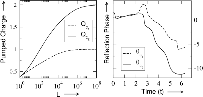
FIG. 6.: $Q$ (in units of $e$) as a function of the RG length scale, $L$ for the two different contours shown in Fig. 4 (triple barrier system). The appropriate reflection phases for the two contours are also shown. We have set $V_{0}=4.5$, $V_{p}=4.0$, and $\delta=\pi/4$ for $C_{1}$ and $\delta=\pi/2$ for $C_{2}$. We have chosen $E_{F}=4.6$. The other parameters are the same as in Fig.(2).

Here, we have computed the $S$-matrix by first obtaining the $M$-matrix for $3$ barriers and obtained the transmission and reflection coefficients, their phases and the pumped charge. The contour plots for the transmission as a function of the barrier heights $V_{1}$ and $V_{2}$ is given in Fig. 5. The four panels which are for four different values of the length scale, starting with the unrenormalised values of the transmission for $L=1$, show how the peaking of the transmission occurs as we go to longer length scales or lower temperatures. As explained in the figure, the maxima ($T$ very close to unity) are shown in black. The separation of transmission between the contours is 0.05 and the lowest value of transmission ($T=0.05$) is for the lightest of the gray contours. The new feature that appears here is the presence of more than one transmission maxima for a given $E_{F}$. Note that the true maxima appear close to the $V_{1}=V_{2}$ line. This is also true for the double barrier case (see Fig. 2). The reason is simply because the transmission maximum (=1) can only be reached for symmetric barriers. Here, the barriers are time- dependent and are not always symmetric, but the maxima still appear when the barriers are symmetric. Note also that in Fig. 5, there are maxima when one of the barrier strengths goes to zero (or one of the barriers is switched off). This is simply the reflection of the resonance maximum of the double barrier case and is not relevant for the genuine triple barrier problem. The pumped charge is now seen to depend on the pumping contour chosen (i.e., the values of the barrier parameters that are modulated). Two possible pumping contours are shown in the Fig. 5, with the solid contour $C_{1}$ enclosing both the transmission maxima and the dashed contour $C_{2}$ only enclosing one. At high temperatures, (first panel in Fig. 5), the regions of non-zero transmission are spread out and the pumped charge can be anything since the dissipation term is large. It cannot be predicted and there is not much difference in the pumped charge of the two contours, which are found to be $Q_{C_{1}}=Q_{C_{2}}=0.38$ for both the curves. But as we decrease the temperature, we see that the regions of high transmission are squeezed together and by the time $L=100$, the two maxima are quite distinct. Both for $L=10$ and for $L=100$, the solid contour $C_{1}$ which encloses more of the areas of non-zero transmission has a higher value of the pumped charge. For the second panel $L=10$, $Q_{C_{1}}=0.73$ and $Q_{C_{2}}=0.57$ and for the third panel,$L=100$, $Q_{C_{1}}=1.12$ and $Q_{C_{2}}=0.72$. By the time $L=10,000$ (at low temperatures), the last panel in Fig. 5 clearly shows that the dashed contour $C_{2}$ encloses all of the transmission around one of the maxima and no part of the transmission of the second maxima. Hence, for this contour, the the charge is quantised to be almost one ($Q_{C_{2}}=0.94$). $C_{1}$, on the other hand, encloses both maxima and most of the non- zero transmission of the second maxima as well. Here, the pumped charge $Q_{C_{1}}=1.7$, and further renormalisation is needed for it to reach the quantisation value of 2. Thus, for the two barrier case, the pumped charge can be quantised to be one or two depending on the pumping contour chosen. This is also shown in Fig.(6), where we also show the change in the reflection phase for both contours. Clearly, the phase change is directly related to the first term in Eq. 7 , and hence to the charge pumped.

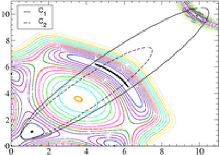
FIG. 7.: Contour plots of the transmission as a function of $V_{1}$ and $V_{2}$ for four barriers. The conventions are the same as in Fig. 5. The two pumping contours have $\delta=\pi/8$, with the solid contour $C_{1}$ having $V_{0}=5.5$ and $V_{p}=5.0$ and the dashed contour $C_{2}$ having $V_{0}=4.0$ and $V_{p}=3.5$. The reflection phases for these contours are shown in Fig.(9).

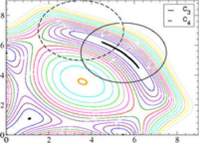
FIG. 8.: Contour plots of the transmission as a function of $V_{1}$ and $V_{2}$ for four barrier with two pumping contours $C_{3}$ enclosing the transmission maximum and $C_{4}$ not enclosing the transmission maximum. $C_{3}$ is defined by $V_{0}=5.5$ and $V_{p}=2.0$ and $C_{4}$ is defined by $V_{01}=3.5,V_{02}=7.0$ and $V_{p}=2.0$. $\delta=\pi/2$ for both contours.

$\bullet$ Triple dot case or $n_{b}=4$ :

Here again, we compute the transmission, the phases and the pumped charge and the contour plots of the transmission are shown in Figs. 7 and 8. The main new feature that appears here is the unusual shape of the resonance maxima - i.e., in one case, it is almost flat in one direction and appears as a line. Also, here, we find that there are three (non-trivial, genuine, quadruple barrier) transmission maxima, which appear along the $V_{1}=V_{2}$ line. (The reason for this has been mentioned earlier. Also, as has been earlier seen, the other maxima that occur for either $V_{1}=0$ or $V_{2}=0$ and are the maxima through triple or double barriers.) The charge pumped is a function of the contour chosen. We can choose a contour that encloses all three maxima, ($C_{1}$ in Fig. 7) or one that only encloses two transmission maxima ($C_{2}$ in Fig. 7). In Fig. (9) , the corresponding phase change in the reflection phase is plotted and we see that depending on whether the contour encloses three or two maxima, the phase change (and consequently, the charge pumped at low temperatures) is three or two units. In Fig. (8), we illustrate yet another important feature. The pumping contour has to actually enclose the centre of the resonance line; otherwise, the pumped charge is zero at low temoeratures. This is seen in Fig. 9, where the phase change for the contour that encloses the central point ($C_{3}$) is shown to be $2\pi$ and the phase change for the contour that does not ($C_{4}$) is shown to be zero.

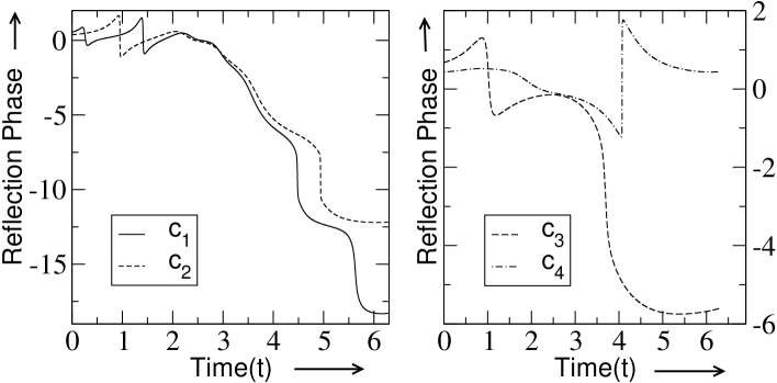
FIG. 9.: The reflection phases as a function of time for the contours shown in Figs. 7 and 8, (four barrier system). $C_{1}$ has a phase drop of $6\pi$, $C_{2}$ has a phase drop of $4\pi$, $C_{3}$ has a phase drop of $2\pi$ and $C_{4}$ has no phase drop. These are correlated with quantised pumped charges of 3, 2, 1 and zero respectively.

These results can easily be extrapolated for the case with arbitrary number of barriers $n_{b}$. The results are very similar. For $n_{b}$ barriers, there are $n_{b}-1$ true maxima close to the $V_{1}\sim V_{2}$ line. If we can choose a pumping contour that encloses all these maxima, the drop in the reflection phase will be $(n_{b}-1)2\pi$ and the maximum pumped charge will be $(n_{b}-1)e$. To obtain quantised values of the charge, we need to go to low temperatures, so that the dissipative term vanishes. However, to obtain the value of the pumped charge at low temperatures, no explicit renormalisation or computation of transmissions at low temperatures need be performed. We only need to compute the change in the reflection phase in one pumping cycle for any given contour. This value is quantised and is a measure of the quantised charge that can be pumped at low temperatures.

Note that all the qualitative features that we have mentioned above for the pumped charge for multiple barriers do not depend on the details of the potentials used, such as the ratio of $V_{p}$ to $V_{0}$, or the value of $E_{f}$ or the value of $a$. We choose $E_{F}\geq V_{i}$ to be in the resonant tunneling limit. Then as we tune the $E_{F}$ for fixed values of the potential, the transmission amplitudes show wide maxima with multiple ($n_{b}-1$) peaks, periodically as a function of $E_{F}$. Similar features are seen for different values of $E_{F}$. Typically, we have chosen $E_{F}$ values where the pumped charge is maximised. Similarly, as a function of the barrier separation $a$, the pumped charge shows periodic behaviour, and we have chosen an arbitrary value of the separation.

Note also that although these results have been obtained for quantum wells, they are also applicable to ‘single level’ quantum dots, where there is only one energy level (close to the Fermi energy) playing a role in the pumping. In other words, as long as the pumping frequency is low, so that $\hbar\omega<\Delta$, where $\Delta$ is the energy separation between the single level and the other levels in the quantum dot, the above analysis should hold.

To conclude, in this paper, we have examined the effects of electron-electron interactions on adiabatic quantum pumps and have shown that the limit of ‘optimal’ quantum pumps ( pumps with no dissipation) are realised at low temperatures, when the effects of interaction drive the dissipative term to zero. We have obtained the scaling of the dissipative term as a function of temperature and shown that it scales as $T^{2\alpha}$ vanishing at $T=0$. Future extensions include the study of interactions on a spin pump[45]

Acknowledgments :

We would like to thank Argha Banerjee for collaboration in the early part of this work and Suryadeep Ray for computational help.

REFERENCES

- [1]
- [2] B. L. Altschuller and L. I. Glazman, Science 283, 1864 (1999).
- [3] D.J. Thouless, Phys. Rev. B27, 6083 (1983).
- [4] Q. Niu, Phys. Rev. B34, 5093 (1986); Phys. Rev. Lett.64, 1812 (1990).
- [5] L.P.Kouwenhoven, A. T. Johnson, N. C. vanderVaart, C. J. P. M. Harmans, C. T. Foxon, Phys. Rev. Lett.67, 1626 (1991).
- [6] H. Pothier et al, Europhys. Lett 17, 249 (1992).
- [7] J. M. Shilton, V. I. Talyanskii, M. Pepper, D. A. Ritchie, J. E. F. Frost, C. J. Ford, C. G. Smith and G. A. C. Jones, J. Phys.: Cond. Matt. 8 L531 (1996).
- [8] M. Switkes et al, Science 283, 1905 (1999).
- [9] P. W. Brouwer, Phys. Rev. B58, R10135 (1998).
- [10] B. Spivak, F. Zhou and M. T. BealMonod, Phys. Rev. B51, 13226 (1995).
- [11] T. A. Shutenko, I. L. Aleiner and B. L. Altshuler, Phys. Rev. B61, 10366 (2000).
- [12] M. Buttiker, A. Pretre and H. Thomas, Z. Phys. B, Cond. Matt. 94, 133 (1994).
- [13] G.Burmeister and and K. Maschke, Phys. Rev. B57, 13050 (1998).
- [14] J. E. Avron, A. Elgart, G. M. Graf and L. Sadun, Phys. Rev. B62, R10618 (2000).
- [15] Y. Levinson, O. Entin-Wohlman and P. Wolfle, Physica A302, 335 (2001).
- [16] O. Entin-Wohlman, A. Aharony and Y. Levinson, Phys. Rev. B65, 195411 (2002).
- [17] Y. Wei, J. Wang and H. Guo, Phys. Rev. B62, 9947 (2000).
- [18] F. Zhou, B. Spivak and B. Altshuler, Phys. Rev. Lett.82, 608 (1999).
- [19] M. L. Polianski and P. W. Brouwer, Phys. Rev. B64, 075304 (2001).
- [20] F. Renzoni and T. Brandes, Phys. Rev. B64, 245301 (2001).
- [21] A. Aharony and O. Entin-Wohlman, Phys. Rev. B65, 241401(R) (2002).
- [22] M. Blaauboer, Phys. Rev. B65, 235318 (2002); M. Blaauboer and E. J. Heller, Phys. Rev. B64, 241301(R) (2001).
- [23] J. N. H. J. Cremers and P. W. Brouwer, Phys. Rev. B65, 115333 (2002).
- [24] M. L. Polianski, M. G. Vavilov, and P. W. Brouwer, Phys. Rev. B65, 245314 (2002).
- [25] M. Moskalets and M. Buttiker, Phys. Rev. B64 201305 (2001); Phys. Rev. B66, 035306 (2002); Phys. Rev. B66, 205320 (2002); Phys. Rev. B68, 161311() (2003); Phys. Rev. B68 075303 (2003); Phys. Rev. B69, 205316 (2004); cond-mat/0407292.
- [26] O.Usmani, E. Lutz and M. Buttiker, Phys. Rev. E 66, 021111 (2002).
- [27] S-L. Zhu, and Z. D. Wang, cond-mat/0208507.
- [28] T. Aono, Phys. Rev. B67, 155303 (2003).
- [29] P. Sharma and P. W. Brouwer,Phys. Rev. Lett.91, 166801 (2003).
- [30] R.Citro, N. Andrei and Q. Niu, cond-mat/0306181.
- [31] A. Banerjee, S. Das and S. Rao, cond-mat/0307324.
- [32] E. Sela and Y. Oreg, cond-mat/0407089.
- [33] I.L. Aleiner and A.V. Andreev, Phys. Rev. Lett.81, 1286 (1998).
- [34] O. Entin-Wohlman and A. Aharony, Phys. Rev. B66, 035329 (2002).
- [35] V. Kashcheyevs, A. Aharony and O. Entin-Wohlman, Phys. Rev. B69, 195301 (2004).
- [36] P. Sharma and C. Chamon, Phys. Rev. Lett.87, 96401 (2001); Phys. Rev. B68,035321 (2003).
- [37] D. Yue, L. I. Glazman and K. A. Matveev, Phys. Rev. B49, 1966, (1994).
- [38] S. Lal, S. Rao and D. Sen, Phys. Rev. B66,165327 (2002)
- [39] D. G. Polyakov and I. V. Gornyi, Phys. Rev. B68, 035421.
- [40] S. Das, S. Rao and D. Sen, Phys. Rev. B70 085318 (2004).
- [41] Q. Niu and D. J. Thouless, J. Phys. A17, 2453 (1984).
- [42] K.A.Matveev, Phys. Rev. B51, 1743 (1995).
- [43] B. Wang, J. Wang and H. Guo, Phys. Rev. B65, 073306 (2002).
- [44] C. L. Kane and M. P. A. Fisher, Phys. Rev. B 46, 15233 (1992).
- [45] Sourin Das and Sumathi Rao, work in progress.