Abstract

The magnetic susceptibility of underdoped yttrium and lanthanum cuprates is interpreted based on the self-consistent solution of the $t$-$J$ model of a Cu-O plane. The calculations reproduce correctly the frequency dependencies of the susceptibility in YBa₂Cu₃O_7-y and La_2-xSr_xCuO₄ attributing their dissimilarity to the difference in the damping of spin excitations. In YBa₂Cu₃O_7-y these excitations are well defined at the antiferromagnetic wave vector ${\bf Q}=(\pi,\pi)$ even in the normal state which manifests itself in a pronounced maximum – the resonance peak – in the susceptibility. In La_2-xSr_xCuO₄ the spin excitations are overdamped which leads to a broad low-frequency feature in the susceptibility. The low-frequency incommensurability in the magnetic response is attributed to a dip in the magnon damping at Q. The calculated concentration and temperature dependencies of the incommensurability parameter conform with experimental observations. Generally the incommensurate magnetic response is not accompanied with an inhomogeneity of the carrier density.

Magnetic Properties of Cuprate Perovskites

1 Introduction

Among the results obtained with inelastic neutron scattering is the detailed information on the magnetic susceptibility in YBa₂Cu₃O_7-y and lanthanum cuprates which reveals a considerable difference in their magnetic properties. A sharp magnetic collective mode – the so-called resonance peak – was observed at frequencies $\omega_{r}=20-40$ meV in YBa₂Cu₃O_7-y and some other cuprates, in underdoped case both below and above $T_{c}$ [1]. In the momentum space the mode is strongly peaked at the antiferromagnetic wave vector ${\bf Q}=(\pi,\pi)$. Contrastingly, no resonance peak was observed in lanthanum cuprates. Instead for low temperatures a broad feature was detected at $\omega_{f}\approx 7$ meV and for this and lower frequencies the susceptibility was found to be peaked at incommensurate momenta $(\pi\pm 2\pi\delta,\pi)$ and $(\pi,\pi\pm 2\pi\delta)$ [2]. Recently the low-frequency incommensurate magnetic response was also observed in YBa₂Cu₃O_7-y [3]. Presently the fundamental difference of the susceptibility frequency dependencies in these two groups of cuprates is actively debated, as well as the nature of the resonance peak and the low-frequency magnetic incommensurability.

The aim of this work is to demonstrate that the above-mentioned unusual properties of cuprates can be interpreted in the framework of the $t$-$J$ model of a Cu-O plane which is a common structure element of these crystals. The model was shown to describe correctly the low-energy part of the spectrum of the realistic extended Hubbard model [4]. To take proper account of strong electron correlations inherent in moderately doped cuprate perovskites the description in terms of Hubbard operators and Mori’s projection operator technique [5] are used. The self-energy equations for hole and spin Green’s functions obtained in this approach are self-consistently solved for the ranges of hole concentrations $0\leq x\lesssim 0.16$ and temperatures 2 K$\leq T\leq$1200 K. Lattices with 20$\times$20 sites and larger are used.

The calculations reproduce correctly the frequency and momentum dependencies of the resonance peak in YBa₂Cu₃O_7-y, and its variation with doping and temperature in normal and superconducting states. The peak is connected with the excitation branch of localized Cu spins and the peak frequency is close to the frequency of these excitations at Q. The absence of the resonance peak in lanthanum cuprates is related to an increased damping of spin excitations which is possibly connected with a large hole damping in these crystals. For low frequencies and temperatures the susceptibility is peaked at incommensurate wave vectors $(\pi\pm 2\pi\delta,\pi)$ and $(\pi,\pi\pm 2\pi\delta)$. The incommensurability is connected with a dip in the magnon damping at Q. In agreement with experiment the incommensurability parameter $\delta$ is approximately proportional to $x$ for $0.02\lesssim x\lesssim 0.12$ and saturates for larger concentrations. The incommensurability disappears with increasing temperature. Generally the incommensurate magnetic response is not accompanied by an inhomogeneity of the carrier density.

2 Main formulas

The Hamiltonian of the two-dimensional $t$-$J$ model reads

$$H=\sum_{\bf nm\sigma}t_{\bf nm}a^{\dagger}_{\bf n\sigma}a_{\bf m\sigma}+\frac{1}{2}\sum_{\bf nm}J_{\bf nm}\left(s^{z}_{\bf n}s^{z}_{\bf m}+s^{+1}_{\bf n}s^{-1}_{\bf m}\right),$$ (1)

where $a_{\bf n\sigma}=|{\bf n}\sigma\rangle\langle{\bf n}0|$ is the hole annihilation operator, n and m label sites of the square lattice, $\sigma=\pm 1$ is the spin projection, $|{\bf n}\sigma\rangle$ and $|{\bf n}0\rangle$ are site states corresponding to the absence and presence of a hole on the site. These states may be considered as linear combinations of the products of the $3d_{x^{2}-y^{2}}$ copper and $2p_{\sigma}$ oxygen orbitals of the extended Hubbard model [6]. We take into account nearest neighbor interactions only, $t_{\bf nm}=-t\sum_{\bf a}\delta_{\bf n,m+a}$ and $J_{\bf nm}=J\sum_{\bf a}\delta_{\bf n,m+a}$ where the four vectors a connect nearest neighbor sites. The spin-$\frac{1}{2}$ operators can be written as $s^{z}_{\bf n}=\frac{1}{2}\sum_{\sigma}\sigma|{\bf n}\sigma\rangle\langle{\bf n}\sigma|$ and $s^{\sigma}_{\bf n}=|{\bf n}\sigma\rangle\langle{\bf n},-\sigma|$.

Properties of the model are determined from the hole and spin retarded Green’s functions

$$G({\bf k}t)=-i\theta(t)\langle\!\{a_{\bf k\sigma}(t),a^{\dagger}_{\bf k\sigma}\}\!\rangle,\quad D({\bf k}t)=-i\theta(t)\langle[s^{z}_{\bf k}(t),s^{z}_{\bf-k}]\rangle,$$ (2)

where $a_{\bf k\sigma}$ and $s^{z}_{\bf k}$ are the Fourier transforms of the respective site operators, operator time dependencies and averaging are defined with the Hamiltonian ${\cal H}=H-\mu\sum_{\bf n}a^{\dagger}_{\bf n\sigma}a_{\bf n\sigma}$ with the chemical potential $\mu$. As mentioned, to obtain self-energy equations for these functions we used Mori’s projection operator technique [5, 7]. In this approach the Fourier transform of Green’s function $\langle\!\langle A_{0}|A^{\dagger}_{0}\rangle\!\rangle$ is represented by the continued fraction

$$\langle\!\langle A_{0}|A^{\dagger}_{0}\rangle\!\rangle=\frac{\displaystyle|A_{0}\cdot A_{0}^{\dagger}|}{\displaystyle\omega-E_{0}-\frac{\displaystyle V_{0}}{\displaystyle\omega-E_{1}-\frac{\displaystyle V_{1}}{\ddots}}}.$$ (3)

The elements of the fraction $E_{i}$ and $V_{i}$ are determined from the recursive procedure

$$[A_{n},H]=E_{n}A_{n}+A_{n+1}+V_{n-1}A_{n-1},$$

$$E_{n}=|[A_{n},H]\cdot A_{n}^{\dagger}|\,|A_{n}\cdot A_{n}^{\dagger}|^{-1},$$ (4)

$$V_{n-1}=|A_{n}\cdot A_{n}^{\dagger}|\,|A_{n-1}\cdot A_{n-1}^{\dagger}|^{-1},\quad V_{-1}=0,\quad n=0,1,2,\ldots$$

The operators $A_{i}$ constructed in the course of this procedure form an orthogonal set, $|A_{i}\cdot A^{\dagger}_{j}|\propto\delta_{ij}$. In Eqs. (3) and (4) the definition of the inner product $|A_{i}\cdot A^{\dagger}_{j}|$ depends on the type of the considered Green’s function. For example, for functions (2) these are $\langle\{A_{i},A^{\dagger}_{j}\}\rangle$ and $\langle[A_{i},A^{\dagger}_{j}]\rangle$, respectively. The method described by Eqs. (3) and (4) can be straightforwardly generalized to the case of many-component operators which is necessary, for example, to consider Green’s functions for Nambu spinors in the superconducting state [7].

The residual term of fraction (3) is the Fourier transform of the quantity

$${\cal T}=|A_{nt}\cdot A_{n}^{\dagger}|\,|A_{n-1}\cdot A_{n-1}^{\dagger}|^{-1},$$ (5)

where the time evolution of the operator $A_{n}$ is determined by the equation

$$i\frac{d}{dt}{A}_{nt}=\prod_{k=0}^{n-1}(1-P_{k})[A_{nt},{\cal H}],\quad A_{n,t=0}=A_{n}$$ (6)

with the projection operators $P_{n}$ defined as $P_{n}Q=|Q\cdot A_{n}^{\dagger}|\,|A_{n}\cdot A_{n}^{\dagger}|^{-1}A_{n}$. The residual term ${\cal T}$ is a many-particle Green’s function which can be estimated by the decoupling. The decoupling is also used in calculating the elements of the continued fractions (3). Following Ref. [8] this approximation is improved by introducing the vertex correction $\alpha$ which is determined from the constraint of zero site magnetization

$$\left\langle s^{z}_{\bf n}\right\rangle=\frac{1}{2}\left(1-x\right)-\left\langle s^{-1}_{\bf n}s^{+1}_{\bf n}\right\rangle=0.$$ (7)

Since the statistical averaging includes samples with different ordering orientations, this condition is fulfilled also in magnetically ordered states.

Equations for Green’s functions obtained in this way for the normal state read [7]

$$G({\bf k}\omega) = \frac{\phi}{\omega-\varepsilon_{\bf k}+\mu-\Sigma({\bf k}\omega)},\;D({\bf k}\omega)=\frac{4(1-\gamma_{\bf k})(J|C_{1}|+tF_{1})}{\omega^{2}-\omega\Pi({\bf k}\omega)-\omega^{2}_{\bf k}},$$

$${\rm Im}\,\Sigma({\bf k}\omega) = \frac{16\pi t^{2}}{N\phi}\sum_{\bf k^{\prime}}\int_{-\infty}^{\infty}d\omega^{\prime}\biggl{[}\gamma_{\bf k-k^{\prime}}+\gamma_{\bf k}+{\rm sgn}(\omega^{\prime})(\gamma_{\bf k-k^{\prime}}-\gamma_{\bf k})$$

$$\times \sqrt{\frac{1+\gamma_{\bf k^{\prime}}}{1-\gamma_{\bf k^{\prime}}}}\biggr{]}^{2}[n_{B}(-\omega^{\prime})+n_{F}(\omega-\omega^{\prime})]$$

$$\times A({\bf k-k^{\prime}},\omega-\omega^{\prime})B({\bf k^{\prime}}\omega^{\prime}),$$

$${\rm Im}\,\Pi({\bf k}\omega) = \frac{9\pi t^{2}J^{2}(1-x)}{2N(1-\gamma_{\bf k})(J|C_{1}|+tF_{1})}\sum_{\bf k^{\prime}}(\gamma_{\bf k+k^{\prime}}-\gamma_{\bf k^{\prime}})^{2}$$

$$\times \int^{\infty}_{-\infty}d\omega^{\prime}A({\bf k^{\prime}}\omega^{\prime})A({\bf k+k^{\prime}},\omega+\omega^{\prime})\frac{n_{F}(\omega+\omega^{\prime})-n_{F}(\omega^{\prime})}{\omega},$$

where $\phi=\frac{1}{2}(1+x)$, $\gamma_{\bf k}=\frac{1}{2}[\cos(k_{x})+\cos(k_{y})]$, $C_{1}=\langle s^{+1}_{\bf n}s^{-1}_{\bf n+a}\rangle$ and $F_{1}=\langle a^{\dagger}_{\bf n}a_{\bf n+a}\rangle$ are the spin and hole correlations on neighboring sites which, as well as the hole concentration $x$, can be calculated from Green’s functions,

$$\omega^{2}_{\bf k}=16J^{2}\alpha|C_{1}|(1-\gamma_{\bf k})(\Delta+1+\gamma_{\bf k}),\;\varepsilon_{\bf k}=-(4\phi t+6C_{1}\phi^{-1}t+3F_{1}\phi^{-1}J)\gamma_{\bf k}$$ (9)

are the energies of spin excitations and holes with the parameter $\Delta$ describing the spin gap at Q, $A({\bf k}\omega)=-\pi^{-1}{\rm Im}\,G({\bf k}\omega)$ and $B({\bf k}\omega)=-\pi^{-1}{\rm Im}\,D({\bf k}\omega)$ are the hole and spin spectral functions, $N$ is the number of sites, $n_{F}(\omega)=[\exp(\omega/T)+1]^{-1}$, $n_{B}(\omega)=[\exp(\omega/T)-1]^{-1}$ with the temperature $T$. Real parts of the self-energies are calculated from their imaginary parts and the Kramers-Kronig relation. The self-energy equations for the superconducting state can be found in Ref. [7].

Equations (7)–(9) form a closed set which can be solved by iteration for fixed chemical potential $\mu$ and temperature $T$. We carried out such calculations for the parameters of the model $J=0.1$ eV, $t=0.5$ eV which correspond to hole-doped cuprates [9]. To stabilize the iteration procedure an artificial damping $i\eta$, $\eta=(0.015-0.05)t$, was added to the frequency in the hole Green’s function.

The results of such calculations can be directly compared with the imaginary part of the magnetic susceptibility $\chi^{\prime\prime}$ derived from the neutron scattering experiments, since this quantity is connected with $B({\bf k}\omega)$,

$$\chi^{\prime\prime}({\bf k}\omega)=4\pi\mu_{B}^{2}B({\bf k}\omega)=-\frac{16\mu_{B}^{2}(1-\gamma_{\bf k})(J|C_{1}|+tF_{1})\omega{\rm Im}\,\Pi}{(\omega^{2}-\omega{\rm Re}\,\Pi-\omega_{\bf k}^{2})^{2}+(\omega{\rm Im}\,\Pi)^{2}},$$ (10)

where $\mu_{B}$ is the Bohr magneton. Equation (10) is the most general form for the magnetic susceptibility which follows from the Mori formalism. With the spin excitation damping $\Pi({\bf k}\omega)$ described by the fermion bubble (LABEL:se) this equation acquires some similarity with the susceptibility derived in the random phase approximation [10] which is frequently used for the discussion of the magnetic properties of cuprates. For this similarity the term $\omega^{2}_{\bf k}$ in the denominator of Eq. (10) has to be negligibly small in comparison with $\omega{\rm Re}\Pi({\bf k}\omega)$. For the hole spectrum self-consistently calculated here this can happen only in the overdoped region $x\gtrsim 0.3$ when the spin correlation $C_{1}$ which determines the magnitude of $\omega_{\bf k}$ [see Eq. (9)] tends to zero [7, 11].

3 The spectrum of spin excitations

As follows from Eq. (10), the frequencies of spin excitations satisfy the equation

$$\omega^{2}-\omega{\rm Re}\,\Pi({\bf k}\omega)-\omega^{2}_{\bf k}=0.$$ (11)

As seen from Eq. (LABEL:se), ${\rm Im}\,\Pi({\bf k}\omega)$ is finite for ${\bf k}\rightarrow 0$, whereas $\omega_{\bf k}$ vanishes in this limit. Therefore the spin Green’s function has a purely imaginary, diffusive pole near the $\Gamma$ point, in compliance with the result of the hydrodynamic theory [12].

The dispersion of spin excitations near Q is of special interest, because this region gives the main contribution into the neutron scattering. This dispersion is shown in Fig. 1.

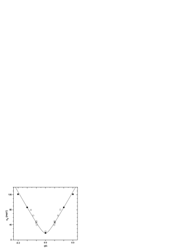
Figure 1: The dispersion of spin excitations near Q along the edge of the Brillouin zone. The dispersion was calculated in a 20$\times$20 lattice for $x=0.06$ and $T=17$ K (filled squares, the solid line is the fit with $\omega_{\bf k}=[\omega^{2}_{\bf Q}+c^{2}({\bf k-Q})^{2}]^{1/2}$). Open squares are the experimental dispersion [1] of the maximum in the frequency dependence of the odd $\chi^{\prime\prime}({\bf q}\omega)$, ${\bf q=k-Q}$, in YBa₂Cu₃O_6.5 ($x\approx 0.075$ [13]) at $T=5$ K.

As seen from this figure, in contrast to the usual spin-wave theory the frequency of spin excitations at the antiferromagnetic wave vector Q is finite. This frequency $\omega_{\bf Q}=4J(2\alpha|C_{1}|\Delta)^{1/2}$ is directly connected with the spin correlation length $\xi$. Indeed, using Eq. (LABEL:se) and taking into account that the region near Q gives the main contribution to the summation over k, we find for large distances and low temperatures

$$\langle s^{z}_{\bf l}s^{z}_{\bf 0}\rangle=N^{-1}\sum_{\bf k}{\rm e}^{i\bf kl}\int_{0}^{\infty}\!\!d\omega\,\coth\left(\frac{\omega}{2T}\right)B({\bf k}\omega)\propto{\rm e}^{i\bf Ql}(\xi/|{\bf l}|)^{1/2}{\rm e}^{-|{\bf l}|/\xi},$$ (12)

where $\xi=\frac{1}{2}a\Delta^{-1/2}$ and $a$ is the distance between in-plane Cu sites. As follows from the calculations, for low concentrations and temperatures $\Delta\approx 0.2x$ and consequently $\xi\approx ax^{-1/2}$. An analogous relation between the spin correlation length and the concentration has been derived from experimental data in La_2-xSr_xCuO₄ [14].

In accord with the Hohenberg-Mermin-Wagner theorem [15] the considered two-dimensional system is in the paramagnetic state for $T>0$. This result can also be obtained using Eq. (LABEL:se). Also it can be shown [7] that in the infinite crystal at $T=0$ the long-range antiferromagnetic order is destroyed for the hole concentrations $x>x_{c}\approx 0.02$.

4 The resonance peak

The imaginary part of the spin susceptibility at the antiferromagnetic wave vector, obtained in our calculations, is shown in Fig. 2.

Figure 2: The imaginary part of the spin susceptibility at Q in the $d$-wave superconducting (a,b) and normal (c,d) states. Curves show the results of our calculations for $\eta=0.015t$, $T=17$ K (a,b) and $T=116$ K (c,d), $x=0.06$ (a,c) and $x=0.12$ (b,d). Squares are the odd susceptibility measured [1] in YBa₂Cu₃O_6.5 ($T_{c}=45$ K, $x\approx 0.075$, a and c) and in YBa₂Cu₃O_6.83 ($T_{c}=85$ K, $x\approx 0.14$ [13], b and d) at $T=5$ K (a,b) and at $T=100$ K (c,d). To depict the experimental data in the same scale they were multiplied by the factor $1.5$.

The experimental data on $\chi^{\prime\prime}$ in YBa₂Cu₃O_7-y [1] are also depicted here. YBa₂Cu₃O_7-y is a bilayer crystal and the symmetry allows one to divide the susceptibility into odd and even parts. The odd part, which for the antiferromagnetic intrabilayer coupling can be compared with our single-layer calculations, is shown in the figure.

The maximum in Fig. 2 is the resonance peak. As seen from this figure, the model reproduces satisfactorily the evolution of the peak position and shape with doping and temperature. In the $t$-$J$ model the peak is connected with the coherent excitations of localized Cu spins near the antiferromagnetic wave vector Q and the peak frequency for ${\bf k=Q}$ is close to the frequency $\omega_{\bf Q}$ in Fig. 1. It is also seen in this figure that the experimental dispersion of the peak is close to the dispersion of the mentioned spin excitations. Thus, we came to conclusion that the resonance peak in YBa₂Cu₃O_7-y and apparently in other cuprate perovskites where it was observed is a manifestation of the magnon branch modified in the short-range antiferromagnetic order.

The above results are related to the underdoped case where the resonance peak is observed both in the normal and superconducting states. In the overdoped case in YBa₂Cu₃O_7-y the peak is observed in the superconducting state only [1]. Calculations for the $t$-$J$ model show that in the normal state on approaching the overdoped region the maximum in $\chi^{\prime\prime}$ rapidly loses its intensity, broadens and shifts to higher frequencies [16]. This result correlates with the broad feature observed experimentally in these conditions. The mechanism of the peak reappearance in the superconducting state in the overdoped region was considered in Ref. [17]. The opening of the $d$-wave superconducting gap with the magnitude $2\Delta^{s}>\omega_{\bf Q}$ decreases considerably the spin excitation damping near Q which restores the peak in $\chi^{\prime\prime}$.

As seen from Fig. 2, the resonance peak has a low-frequency shoulder which is more pronounced for low concentrations and temperatures. The shoulder stems from the frequency dependence of the magnon damping ${\rm Im}\,\Pi({\bf Q}\omega)$ which in its turn is a consequence of the hole Fermi surface nesting existing in the $t$-$J$ model for moderate doping [7]. An analogous nesting is expected in the two-layer YBa₂Cu₃O_7-y between the parts of the Fermi surface belonging to the bonding and antibonding bends [10].

It is worth noting that for all four curves in Fig. 2 the value of $|\Pi({\bf Q},\omega_{\bf Q})|/2$ is smaller than $\omega_{\bf Q}$. The satisfactory agreement between the experimental and calculated results allows us to conclude that near Q the spin excitations are not overdamped in underdoped YBa₂Cu₃O_7-y. In calculating the curves in Fig. 2 the artificial broadening $\eta$ in the hole Green’s function was set equal to $0.015t$. This broadening simulates contributions to the hole damping from mechanisms differing from the spin excitation scattering. The magnitude of these interactions can essentially vary in different crystals. The example of the magnetic susceptibility calculated with the larger hole damping $\eta=0.05t$ is shown in Fig. 3.

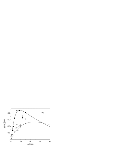
Figure 3: The frequency dependence of the imaginary part of the susceptibility. (a) The solid line corresponds to $T=29$ K, $\eta=0.05t$ and $x\approx 0.1$. The dashed line is for $T=116$ K and the same other parameters. Symbols are experimental results [2] in La_1.86Sr_0.14CuO₄ at $T=35$ K (filled circles) and $T=80$ K (open circles). Vertical bars show experimental errors. The calculated susceptibility is given for ${\bf k}={\bf Q}$, the experimental data are for a wave vector of the incommensurate peak. (b) The solid line is the same as in part (a). The dashed line is calculated for $\eta=0.015t$, other parameters are the same as for the solid line.

As seen from this figure, the spin excitation damping is very sensitive to the hole damping. The increase of this latter damping leads to a marked growth of the spin excitation damping which results in the overdamping of these excitations. Instead of the pronounced peak at the frequency $\omega_{\bf Q}$ a broad low-frequency feature is observed in the susceptibility (see Fig. 3b). This shape resembles that observed in La_2-xSr_xCuO₄ [2]. The comparison was carried out in Fig. 3a. It should be noted that the use of a comparatively small 20$\times$20 lattice did not allow us to describe the incommensurability of the magnetic response – $\chi^{\prime\prime}$ is peaked at Q and our calculated data belong to this momentum (the use of a larger lattice is too time-consuming for the self-consistent calculations). In La_1.86Sr_0.14CuO₄ the low-frequency susceptibility is peaked at incommensurate momenta ${\bf k}=(\pi\pm 2\pi\delta,\pi),(\pi,\pi\pm 2\pi\delta)$ and the experimental data [2] shown in Fig. 3a belong to one of these momenta. These data were increased by approximately 2.5 times to show them in the scale with the calculated results. The need for scaling is apparently connected with the splitting of the commensurate peak into the four incommensurate maxima. Apart from this difference in the momentum dependencies, the calculated frequency and temperature dependencies are in good agreement with the experimental results. Thus, it can be concluded that the dissimilarity of the frequency dependencies of the susceptibility in YBa₂Cu₃O_7-y and La_2-xSr_xCuO₄ is connected with different values of the damping of spin excitations, which are well defined at the antiferromagnetic wave vector in the former crystal and overdamped in the latter. This property of spin excitations in La_2-xSr_xCuO₄ is not changed in the superconducting state due to the small superconducting gap $2\Delta^{s}\approx 9{\rm meV}<\omega_{\bf Q}$ in this crystal [17].

5 Incommensurability in the magnetic response

For low frequencies susceptibility (10) is essentially simplified,

$$\chi^{\prime\prime}({\bf k}\omega)\propto\frac{\omega{\rm Im}\Pi({\bf k}\omega)}{\omega^{4}_{\bf k}}.$$ (13)

As seen from Fig. 1 and Eq. (9), $\omega_{\bf k}$ is the increasing function of the difference ${\bf k-Q}$ and therefore the denominator of the fraction (13) favors the appearance of a commensurate peak centered at the antiferromagnetic momentum in the susceptibility. However, if the spin excitation damping has a pronounced dip at ${\bf k=Q}$ the peak splits into several peaks shifted from Q. To make sure that the damping may really have such a behavior let us consider the case of low hole concentrations and temperatures. In this case the hole Fermi surface consists of four ellipses centered at $(\pm\pi/2,\pm\pi/2)$ [7]. Two of them are shown in Fig. 4.

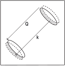
Figure 4: The Brillouin zone of the square lattice. Solid curves are two of four ellipses forming the Fermi surface at small $x$. Dashed lines are the Fermi surface contours shifted by $\pm({\bf k-Q})$. Regions of ${\bf k^{\prime}}$ and ${\bf k+k^{\prime}}$ contributing to the damping (14) are shaded.

The spin excitation damping described by the fermion bubble (LABEL:se) is simplified to

$${\rm Im}\,\Pi({\bf k}\omega) \propto \sum_{\bf k^{\prime}}(\gamma_{\bf k^{\prime}}-\gamma_{\bf k^{\prime}+k})^{2}\Big{[}n_{F}(\varepsilon_{\bf k^{\prime}+k}-\mu)-n_{F}(\varepsilon_{\bf k^{\prime}}-\mu)\Big{]}$$ (14)

$$\times \delta(\omega+\varepsilon_{\bf k^{\prime}}-\varepsilon_{\bf k^{\prime}+k})$$

in the considered case. Here $\varepsilon_{\bf k}$ is the hole dispersion. In the process described by Eq. (14) a fermion picks up an energy and momentum of a defunct spin excitation and is transferred from a region below the Fermi level to a region above it. However, for ${\bf k=Q}$ this process is impossible, because for initial states ${\bf k^{\prime}}$ interior to an ellipse in Fig. 4 all final states with momenta ${\bf k+k^{\prime}}$ will be inside another ellipse, i.e. below the Fermi level. Thus, in this simplified picture the damping vanishes for ${\bf k=Q}$ and grows with increasing the difference ${\bf k-Q}$ approximately proportional to the shaded area in Fig. 4 [18].

With increasing the hole concentration the Fermi surface of the $t$-$J$ model is transformed to a rhombus centered at Q [16]. This result is in agreement with the Fermi surface observed in La_2-xSr_xCuO₄ [19] [however, to reproduce the experimental Fermi surface terms describing the hole transfer to more distant coordination shells have to be taken into account in the kinetic term of Hamiltonian (1)]. For such $x$ another mechanism of the dip formation in the damping comes into effect. The interaction constant $\gamma_{\bf k^{\prime}}-\gamma_{\bf k^{\prime}+k}$ in Eq. (14) vanishes in the so-called “hot spots” – the crossing points of the Fermi surface with the boundary of the magnetic Brillouin zone. For small frequencies and ${\bf k=Q}$ the nearest vicinity of these points contributes to the damping. Consequently, the damping has a dip at Q. With the inclusion of the hole transfer to more distant coordination shells the interaction constant is changed, however the conclusion about the dip at the antiferromagnetic momentum in the damping remains unchanged.

The dip disappears when the hole damping $\eta$ exceeds the frequency $\omega>0$. Since the main contribution to the damping is made by states with energies $-\omega\leq\varepsilon_{\bf k^{\prime}}-\mu\leq 0$ and $0\leq\varepsilon_{\bf k^{\prime}+k}-\mu\leq\omega$, this means that the above consideration is valid when there exist well defined quasiparticle excitations near the Fermi surface.

Results of our calculations in a 120$\times$120 lattice and experimental data are shown in Fig. 5.

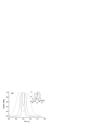
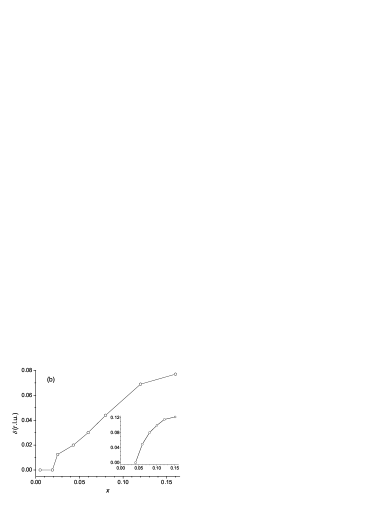
Figure 5: (a) The dynamic structure factor vs. wave vector along the edge of the Brillouin zone for $x=0.015$ (solid line), 0.06 (dashed line), and 0.12 (short dash). For all curves $T=58$ K and $\omega=2$ meV. Inset: the structure factor measured [20, 21] in La_2-xSr_xCuO₄ for $x=0.03$, $T=2$ K, $\omega=0$ (filled squares and solid line), $x=0.06$, $T=25$ K, $\omega=2$ meV (triangles and dashed line), and $x=0.12$, $T=31$ K, $\omega=2$ meV (open squares and short dash). Fitting curves in the inset are from Refs. [20, 21]. (b) The incommensurability parameter $\delta$ vs. $x$ for $T=58$ K and $\omega=2$ meV. Inset: experimental data [20] for La_2-xSr_xCuO₄. The wave vector and the incommensurability parameter are given in the reciprocal lattice units $2\pi/a$.

In agreement with experiment [20, 22] in our calculations peaks in the dynamic structure factor $S({\bf k}\omega)=[1-\exp(-\omega/T)]^{-1}\chi^{\prime\prime}({\bf k}\omega)$ along the edge of the Brillouin zone [the direction $(\pi,\pi)-(0,\pi)$] are more intensive than those along the diagonal [the direction $(\pi,\pi)-(0,0)$]. As seen from Fig. 5, the calculations reproduce correctly the main known features of the incommensurate response except that the experimental $\delta$ is somewhat larger than the calculated one. In experiment with increasing $T$ the incommensurability decreases and finally disappears. The calculations reproduce this peculiarity also. In the calculations the concentration dependence of $\delta$ is mainly determined by the spin gap parameter $\Delta$ in $\omega_{\bf k}$ in Eq. (9). For $x<0.12$ it grows with $x$ and saturates at larger concentrations [7].

With increasing $\omega$ the dip in the spin excitation damping is shallowed and finally disappears. Besides, on approaching $\omega_{\bf Q}$ the denominator in Eq. (10) will favor the appearance of the commensurate peak at Q. Thus, the low-frequency incommensurate maxima of $\chi^{\prime\prime}$ converge to the commensurate peak at $\omega\approx\omega_{\bf Q}$. The dispersion of the maxima in $\chi^{\prime\prime}$ above $\omega_{\bf Q}$ is determined by the denominator in Eq. (10) and is close to that shown in Fig. 1. Consequently, the dispersion of the maxima in $\chi^{\prime\prime}$ resembles two parabolas converging near the point $({\bf Q},\omega_{\bf Q})$. The upper parabola with branches pointed up reflects the dispersion of spin excitations, while the lower parabola with branches pointed down stems from the momentum dependence of the spin excitation damping. Such kind of the dispersion is indeed observed in cuprates [3, 23].

Generally the incommensurate magnetic response is not accompanied by an inhomogeneity of the carrier density. In works based on the stripe mechanism [23] the magnetic incommensurability is connected with the appearance of a charge density wave. Notice however, that the magnetic incommensurability is observed in all lanthanum cuprates, while the charge density wave is detected in neutron scattering in those cuprates which are in the low-temperature tetragonal or less-orthorhombic phases (La_2-xBa_xCuO₄, La_2-y-xNd_ySr_xCuO₄) [24]. In these phases the charge density wave is stabilized by the corrugated pattern of the in-plane lattice potential. It can be supposed that the magnetic incommensurability may be a precursor rather than a consequence of the charge density wave.

6 Concluding remarks

In this paper the projection operator technique was used for investigating the magnetic properties of the $t$-$J$ model of cuprate high-$T_{c}$ superconductors. It was demonstrated that the calculations reproduce correctly the frequency and momentum dependencies of the experimental magnetic susceptibility and its variation with doping and temperature in the normal and superconducting states in YBa₂Cu₃O_7-y and lanthanum cuprates. This comparison with experiment allowed us to associate the resonance peak in YBa₂Cu₃O_7-y with the magnon branch modified in the short-range antiferromagnetic order. The lack of the resonance peak in La_2-xSr_xCuO₄ was connected with an increased damping of spin excitations at the antiferromagnetic wave vector ${\bf Q}=(\pi,\pi)$. One of the possible reasons for the overdamped excitations is an increased hole damping in this crystal. It was shown that for low frequencies the susceptibility is peaked at incommensurate momenta $(\pi\pm 2\pi\delta,\pi)$ and $(\pi,\pi\pm 2\pi\delta)$. The incommensurability is the consequence of the dip in the momentum dependence of the spin excitation damping at Q. The dip appears due to the Fermi surface nesting for low hole concentrations $x$ and due to small hole-magnon interaction constants for moderate concentrations. In agreement with experiment for $x\lesssim 0.12$ the incommensurability grows nearly proportional to $x$ and tends to saturation for $x>0.12$. This is connected with the concentration dependence of the spin excitation frequency at Q. Also in agreement with experiment the incommensurability decreases with increasing temperature. The dispersion of the maxima in the susceptibility resembles two converging parabolas. The upper parabola with branches pointed up reflects the dispersion of spin excitations, while the lower parabola with branches pointed down stems from the momentum dependence of the spin excitation damping. In the considered mechanism the magnetic incommensurability is not accompanied by the inhomogeneity of the carrier density.

99

References

- [1] P. Bourges, in The Gap Symmetry and Fluctuations in High Temperature Superconductors, edited by J. Bok, G. Deutscher, D. Pavuna, and S. A. Wolf (Plenum Press, 1998), p. 349; H. He, Y. Sidis, P. Bourges, G. D. Gu, A. Ivanov, N. Koshizuka, B. Liang, C. T. Lin, L. P. Regnault, E. Schoenherr, and B. Keimer, Phys. Rev. Lett. 86, 1610 (2001).
- [2] G. Aeppli, T. E. Mason, S. M. Hayden, H. A. Mook, and J. Kulda, Science 279, 1432 (1997).
- [3] M. Arai, T. Nishijima, Y. Endoh, T. Egami, S. Tajima, K. Tamimoto, Y. Shiohara, M. Takahashi, A. Garrett, and S. M. Bennington, Phys. Rev. Lett. 83, 608 (1999); D. Reznik, P. Bourges, L. Pintschovius, Y. Endoh, Y. Sidis, T. Matsui, and S. Tajima, cond-mat/0307591.
- [4] F. C. Zhang and T. M. Rice, Phys. Rev. B 37, 3759 (1988).
- [5] H. Mori, Progr. Theor. Phys. 34, 399 (1965); A. V. Sherman, J. Phys. A 20, 569 (1987).
- [6] J. H. Jefferson, H. Eskes, L. F. Feiner, Phys. Rev. B 45, 7959 (1992); A. V. Sherman, Phys. Rev. B 47, 11521 (1993).
- [7] A. Sherman and M. Schreiber, Phys. Rev. B 65, 134520 (2002); 68, 094519 (2003); Eur. Phys. J. B 32, 203 (2003).
- [8] J. Kondo and K. Yamaji, Progr. Theor. Phys. 47, 807 (1972); H. Shimahara and S. Takada, J. Phys. Soc. Jpn. 61, 989 (1992); S. Winterfeldt and D. Ihle, Phys. Rev. B 58, 9402 (1998).
- [9] A. K. McMahan, J. F. Annett, and R. M. Martin, Phys. Rev. B 42, 6268 (1990); V. A. Gavrichkov, S. G. Ovchinnikov, A. A. Borisov, and E. G. Goryachev, Zh. Eksp. Teor. Fiz. 118, 422 (2000) [JETP (Russia) 91, 369 (2000)].
- [10] D. Z. Liu, Y. Zha, and K. Levin, Phys. Rev. Lett. 75, 4130 (1995); N. Bulut and D. J. Scalapino, Phys. Rev. B 53, 5149 (1996).
- [11] J. Bonča, P. Prelovšek, and I. Sega, Europhys. Lett. 10, 87 (1989).
- [12] D. Forster, Hydrodynamic Fluctuations, Broken Symmetry, and Correlation Functions (W. A. Benjamin, Inc., London, 1975).
- [13] J. L. Tallon, C. Bernhard, H. Shaked, R. L. Hitterman, and J. D. Jorgensen, Phys. Rev. B 51, 12911 (1995).
- [14] B. Keimer, N. Belk, R. G. Birgeneau, A. Cassanho, C. Y. Chen, M. Greven, M. A. Kastner, A. Aharony, Y. Endoh, R. W. Erwin and G. Shirane, Phys. Rev. B 46, 14034 (1992).
- [15] N. D. Mermin and H. Wagner, Phys. Rev. Lett. 17, 1133 (1966); P. C. Hohenberg, Phys. Rev. 158, 383 (1967).
- [16] A. Sherman, cond-mat/0409379.
- [17] D. K. Morr and D. Pines, Phys. Rev. Lett. 81, 1086 (1998).
- [18] A. Sherman and M. Schreiber, Phys. Rev. B 69, 100505(R) (2004); A. Sherman, phys. status solidi (b) 241, 2097 (2004).
- [19] X. J. Zhou, T. Yoshida, D.-H. Lee, W. L. Yang, V. Brouet, F. Zhou, W. X. Ti, J. W. Xiong, Z. X. Zhao, T. Sasagawa, T. Kakeshita, H. Eisaki, S. Uchida, A. Fujimori, Z. Hussain, and Z.-X. Shen, cond-mat/0403181.
- [20] K. Yamada, C. H. Lee, K. Kurahashi, J. Wada, S. Wakimoto, S. Ueki, H. Kimura, Y. Endoh, S. Hosoya, G. Shirane, R. J. Birgeneau, M. Greven, M. A. Kastner, and Y. J. Kim, Phys. Rev. B 57, 6165 (1998).
- [21] S. Wakimoto, G. Shirane, Y. Endoh, K. Hirota, S. Ueki, K. Yamada, R. J. Birgeneau, M. A. Kastner, Y. S. Lee, P. M. Gehring, S. H. Lee, Phys. Rev. B 60, R769 (1999).
- [22] H. Yoshizawa, S. Mitsuda, H. Kitazawa, and K. Katsumata, J. Phys. Soc. Jpn. 57, 3686 (1988); R. J. Birgeneau, Y. Endoh, Y. Hidaka, K. Kakurai, M. A. Kastner, T. Murakami, G. Shirane, T. R. Thurston, and K. Yamada, Phys. Rev. B 39, 2868 (1989).
- [23] J. M. Tranquada, H. Woo, T. G. Perring, H. Goka, G. D. Gu, G. Xu, M. Fujita, and K. Yamada, Nature 429, 534 (2004).
- [24] M. Fujita, H. Goka, K. Yamada, and M. Matsuda, Phys. Rev. Lett. 88, 167008 (2002).