A Monte Carlo Investigation of the Hamiltonian Mean Field Model

Abstract

We present a Monte Carlo numerical investigation of the Hamiltonian Mean Field (HMF) model. We begin by discussing canonical Metropolis Monte Carlo calculations, in order to check the caloric curve of the HMF model and study finite size effects. In the second part of the paper, we present numerical simulations obtained by means of a modified Monte Carlo procedure with the aim to test the stability of those states at minimum temperature and zero magnetization (homogeneous Quasi Stationary States) which exist in the condensed phase of the model just below the critical point. For energy densities smaller than the limiting value $U\sim 0.68$, we find that these states are unstable confirming a recent result on the Vlasov stability analysis applied to the HMF model.

, ,

1 Introduction

The Hamiltonian Mean Field (HMF) model, introduced in ref. [1, 2] is a classical many-body model of fully-coupled rotators, that has recently raised a great interest for its connections to nonextensive thermodynamics [3, 4, 5, 6, 7, 8, 9] and glassy systems [10, 11]. It can be seen as a system of $N$ planar classical inertial spins ${\stackrel{{\scriptstyle\vector(1,0){8.0}}}{{s_{i}}}}=(cos\theta_{i},sin\theta_{i})$ which interact through an infinite-range potential or equivalently as $N$ interacting particles moving on the unit circle [2]. Indicating with $K$ the kinetic energy and with $V$ the potential energy, the Hamiltonian can be written as

$$H=K+V=\sum_{i=1}^{N}{{p_{i}}^{2}\over 2}+{1\over{2N}}\sum_{i,j=1}^{N}[1-cos(\theta_{i}-\theta_{j})]~{}~{},$$ (1)

where $-{\pi}\leq{\theta_{i}}<{\pi}$ is the $ith$ angle and $p_{i}$ the corresponding conjugate momentum. The degree of clustering of the system can be expressed through the usual order parameter M, defined as

$$M={1\over{N}}|\sum_{i=1}^{N}\stackrel{{\scriptstyle\vector(1,0){8.0}}}{{s_{i}}}|~{}~{}~{}~{}.$$ (2)

The model can be solved exactly in the canonical ensemble formalism and exhibits a second-order phase transition from a low-energy condensed (ferromagnetic) phase with magnetization $M\neq 0$, to a high-energy homogeneous one (paramagnetic), with $M=0$. The dependence of the temperature $T={2<K>\over N}$ on the energy density $U=E/N$ at equilibrium is given by the following caloric curve [1, 2]

$$U={T\over 2}+{1\over 2}\left(1-M^{2}\right)~{}.$$ (3)

The critical point is at energy density $U_{c}=0.75$ and the corresponding critical temperature is $T_{c}=0.5$. The dynamics of HMF can be investigated by numerical integration of the equations of motion at constant energy. Starting the system with out-of-equilibrium initial conditions, for example adopting the so-called M1 initial conditions (i.e. considering $\theta_{i}=0$ for all $i$ - so that $M(t=0)=1$ - and velocities uniformly distributed), the results of the microcanonical molecular dynamics (MD) simulations show a disagreement with the canonical prediction in a region of energy values $0.5<U<U_{c}$ [3, 5, 8]. Here, for a transient regime whose length depends on the size N, the system remains trapped in anomalous metastable quasi-stationary states (QSS) at a temperature lower then the canonical equilibrium one. After such a transient, for a finite size N, the system slowly relaxes towards Boltzmann-Gibbs (BG) equilibrium, showing aging and power-law correlations [8]. Moreover, in the thermodynamic limit, if the infinite time limit is considered after $N\rightarrow\infty$, the quasi-stationary states become stable and the QSS regime can be considered as a true non-canonical equilibrium phase of the model [3]. In the last years many investigations have been performed in order to explain the nature of the dynamically-generated anomalies of the QSS regime. The most promising scenarios seem to be Tsallis nonextensive statistical mechanics framework [3, 5, 8] and the glassy-like weak ergodicity breaking description [10, 11]. Both of these scenarios indicate that, during the QSS regime, the system remains trapped in a very complex (fractal) region of the phase space, which hinders the complete visit of the whole a-priori accessible phase space.
In this paper we present a Monte Carlo study of the HMF model. In fact an extensive Monte Carlo investigation is missing in the literature and only in refs. [12, 13] some calculations for very small sizes were discussed. The present paper is divided into two sections. In the first one, by means of a standard Metropolis algorithm, we reproduce the canonical equilibrium caloric curve of the model and study finite size effects close to the critical point where fluctuations are larger and simulations more delicate. In the second section, we modify the standard algorithm in order to perform a sampling over the constant energy hypersurface of phase space, looking for those states with minimum temperature (kinetic energy), not necessarily Boltzmann-Gibbs equilibrium states. Below the critical energy $U_{c}=0.75$ density, these spatially homogeneous $(M=0)$ states coincides with the microcanonical non-equilibrium QSS for energy greater than $U\sim 0.68$. With our modified Monte Carlo algorithm we found that below this limiting value, as also showed in a recent paper [15] by means of a nonlinear stability test, the homogeneous states are effectively unstable. We discuss these results comparing them with the out-of-equilibrium caloric curve calculated using molecular dynamics and with the absolute minimum temperature curve.

2 Metropolis Monte Carlo simulations

The Metropolis Monte Carlo algorithm is a well-known general method [14] for computing the canonical equilibrium statistical expectation values by means of a weigthed random sampling of the possible microstates. The algorithm usually generates a Markov chain of configurations, for which the probability of having a given configuration $C_{n}$ depends only on $C_{n-1}$ and not on the previous history of the system. Given a configuration $C_{n}$, one extracts a new trial configuration $C^{\prime}$ with a random algorithm characterized by a simmetric transition probability, in order to satisfy the detailed balance condition and to minimize the free energy. For example, in the Ising model the configuration $C^{\prime}$ could be the configuration $C_{n}$ in which a random chosen spin has been flipped. More generally, the configuration $C^{\prime}$ could be obtained from $C_{n}$ by changing at random the state of the $ith$ spin of the system considered. Then, if the equilibrium distribution is $exp[-\beta H(C)]$, where $H(C)$ is the Hamiltonian of the system and $\beta$ the inverse of the temperature T (which remains constant), one computes $H(C^{\prime})-H(C_{n})\equiv\Delta H$ and uses the extraction of a uniformly distributed random number $r$ in the interval [0,1] in order to accept the new configuration, according to the following rules

$$C_{n+1}=C_{n}~{}~{}~{}~{}~{}~{}~{}if~{}~{}~{}exp[-\beta\Delta H]<r$$

$$C_{n+1}=C^{\prime}~{}~{}~{}~{}~{}~{}~{}if~{}~{}~{}exp[-\beta\Delta H]>r~{}~{},$$ (4)

By means of this technique one can generate a sequence of configurations from which, after an opportune thermalization transient, it is possible to get the canonical equilibrium properties of the system. In fact, if $N_{iter}$ is the number of iterations of the algorithm, the expectation value of any observable quantity $A(C)$ can be calculated using the identity

$$\lim_{N_{iter}\rightarrow\infty}\frac{1}{N_{t}}\sum_{n=1}^{N_{iter}}A(C_{n})=\int d\mu(C)A(C),$$ (5)

with

$$d\mu(C)\sim exp[-\beta H(C)],~{}~{}~{}~{}~{}~{}~{}\int d\mu(C)=1~{}~{}.$$ (6)

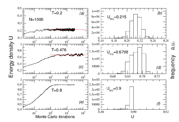
Figure 1: For the case $N=1000$ we plot in panels (a), (c), (e) the standard Metropolis Monte Carlo evolution of the energy density U and the relative histograms, in panels (b), (d), (f) for three different values of temperature, i.e. $T=0.2,0.476,0.8$, which are , respectively, below, near and above the phase transition.

At variance with usual statistical models, the HMF model has also a kinetic term. Thus in order to use the standard Metropolis algorithm and calculate the caloric curve of the HMF model, we fixed the parameter $\beta=1/T$, in this way the kinetic energy $K=NT/2$ of the system of N rotators is fixed as well and remains constant for all the simulation. We started from initial conditions with all the angles equal to zero, i.e. $M(t=0)\sim 1$. Then , in the configuration $C_{n}$, we changed the angle $\theta_{k}$ of a given small quantity (choosen properly in order to satisfy the detailed balance condition), so that, in the new configuration $C^{\prime}$, we have $\theta^{\prime}_{k}=\theta_{k}+\Delta\theta_{k}$. We computed the corresponding variation $\Delta V$ in the potential energy and since $\Delta K=0$ we have $\Delta H=\Delta V$. Following the rule of eq. (4) we finally accepted or not the new configuration. After a termalization transient, we started to compute the average energy density $U=H/N$ by means of eq.(5).

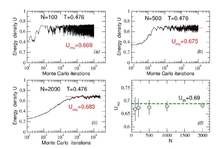
Figure 2: For the case $T=0.476$ which corresponds to the well studied energy density value $U=0.69$, we plot in panels (a), (b) and (c) the standard Metropolis Monte Carlo evolution for different $N$ in order to investigate finite size effects. The average value $U_{mc}$ is also reported and shown as dashed line. In panel (d) we plot the values of the energy density obtained as a function of the system size. A clear convergence towards the theoretical prediction $U_{th}$ is evident together with a decrease of the error bar which is given by the corresponding standard deviation extracted from the numerical fluctuations around the average value.

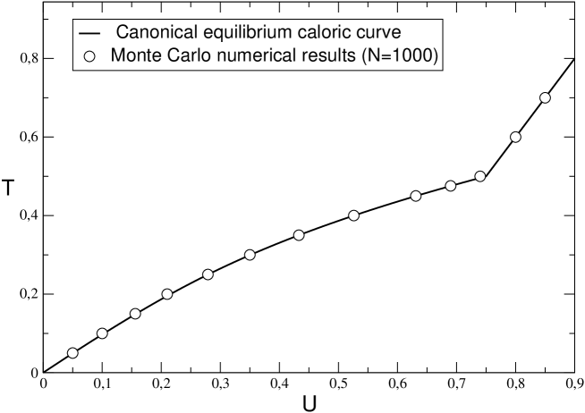
Figure 3: The numerical results of the standard Metropolis simulations performed for a system of N=1000 rotators (circles) are plotted in comparison with the analytical canonical caloric curve, corresponding to the Boltzmann-Gibbs equilibrium (full curve).

Let us discuss in the following the numerical results obtained with this standard Monte Carlo algorithm. In Fig.1,panels (a), (c) and (e), we plot Metropolis simulations performed for a system of N=1000 rotators and three different values of temperatures. We considered in particular the values $T=0.2,0.476,0.8$ which are, respectively, below, near and above the phase transition crtitical temperature $T_{c}=0.5$. After a transient time, the simulations converge to a plateau and fluctuate around an average value. We report in panels (b), (d) and (f) the relative histograms with the average Monte Carlo values $U_{mc}$ obtained. As expected, fluctuations are larger for temperatures close to the critical one.

In order to study finite size effects and fluctuations we discuss the evolution for different system sizes at a temperature just below $T_{c}$. We considered the case $T=0.476$ which should correspond to the well known energy density $U=0.69$. In Fig.2 (a), (b) and (c), we show the Monte Carlo evolution for this case for different sizes of the system. While fluctuations are quite consistent for $N=100$, they diminish as expected with the size of the system. Also the value to which the simulation finally converges gets closer to the theoretical prediction the bigger the size of the system. This is evident in panel (d) of the same figure where the values obtained for different numbers of rotators together with the relative standard deviations are plotted in comparison with the theoretical expected one.

Finally, in Fig.3, we plot the average energy densities obtained with the Monte Carlo simulations for a wide range of temperature values. The Monte Carlo points are compared with the analytical canonical curve (full curve) corresponding to the Boltzmann-Gibbs equilibrium [1, 2]. The agreement is very good for this energy size (N=1000). As expected at equilibrium, where ergodicity should be satisfied no anamalies are found. A similar results was obtained for microcanonical Monte Carlo simulations [12, 13]. On the other hand, as discussed in refs. [3, 4, 5, 6, 8], the origin of the anomalies is in the dynamics which induces frustration and nonergodicity for a transient time - before complete equilibration - which diverges with $N$. In order to try to shed more light on these metastable states we modified the standard Monte Carlo algorithm as explained in the next section.

3 Monte Carlo optimization at constant Energy

3.1 The algorithm

We mentioned in the introduction that the so-called QSS, i.e. the out-of-equilibrium metastable states that emerge from the microcanonical molecular dynamics simulations, become stationary in the thermodynamic limit and lie at temperature lower than the canonical equilibrium one. More precisely, up to $U\sim 0.68$, the QSS points lie on the extension, in the condensed phase, of the high temperature line of the caloric curve (this line is the geometric place of states with M=0, maximum potential energy and minimum kinetic one). This means that the homogeneous quasi-stationary non-equilibrium states with zero magnetization should be stable only up to those limiting values, but not below. In a recent paper on the HMF model [15], the authors apply a nonlinear stability criterion (a modification of that one originally proposed in ref. [16]) to a selected set of spatially homogeneous solutions of the Vlasov equation, which describes the continuum limit of the Hamiltonian Mean Field model. Actually these solutions are qualitatively very similar to the zero magnetization QSS arising from the microcanonical simulations with M1 initial conditions and also the results of the stability test found in [15] were consistent with the numerical evidence of the disappearance of the homogeneous QSS family below $U\sim 0.68$.
With the aim to study these anamalous states without using molecular dynamics tecniques, but only performing a sampling over the constant energy density hypersurface in phase space, we modified the standard MC Metropolis algorithm adopted in section 2. Our purpose was not that one of finding Boltzmann-Gibbs equilibrium configurations, on the other hand we wanted to select those out-of-equilibrium configurations which minimize the temperature (i.e. the kinetic energy) of the system at constant total energy, in order to look for homogeneous QSS’s close to the critical point and study their eventual stability. The problem is an optimization-like one, i.e. using a Monte Carlo procedure, one wants to find the states at minimal temperature with the constraint of total energy conservation.

The new algorithm we have adopted obeys the following rules:

1. It starts from initial conditions with fixed magnetization and momenta uniformly distributed. Then randomly changes the momentum $p_{k}$ in the configuration $C_{n}$ so that $p_{k}+\Delta p_{k}=\Pi$; thus, in the new configuration $C^{\prime}$, one has

   $$p^{\prime}_{i}=p_{i}+(\Pi-p_{i})\delta_{i,k}~{}~{}~{}~{}~{}~{}~{}with~{}~{}~{}i=1,....,N;$$

2. it computes the corresponding variation in the kinetic energy

   $$K^{\prime}=\frac{1}{2}\sum_{i=1}^{N}[p_{i}^{2}+(\Pi^{2}-p_{i}^{2})\delta_{i,k}]=K+\frac{1}{2}\Pi^{2}-\frac{1}{2}p_{k}^{2}~{}\Longrightarrow$$

   $$\Longrightarrow~{}\Delta K=\frac{1}{2}\Pi^{2}-\frac{1}{2}p_{k}^{2}$$

3. then the $n+1$ configuration is

   $$C_{n+1}=C_{n}~{}~{}~{}~{}~{}~{}~{}if~{}~{}~{}exp[-2\Delta K]<r$$

   $$C_{n+1}=C^{\prime}~{}~{}~{}~{}~{}~{}~{}if~{}~{}~{}exp[-2\Delta K]>r$$ (7)

   where $r$ is the usual random number chosen uniformly in the interval [0,1];

4. finally, if the new configuration $C^{\prime}$ is accepted, it calculates the new value $\Theta$ of the angle $\theta_{k}$ by means of the variation of the potential energy $\Delta V=-\Delta K$, knowing that

   $$V^{\prime}=V+\Delta V=\frac{1}{2N}\sum_{i,j=1}^{N}[1-\cos(\theta^{\prime}_{i}-\theta^{\prime}_{j})]$$ (8)

   and

   $$\theta^{\prime}_{i}=\theta_{i}+(\Theta-\theta_{i})\delta_{i,k}~{}~{}~{}~{}~{}~{}~{}~{}~{}~{}i=1,....,N~{}.$$

   After some algebra, one finally obtains the following equation for $\Theta$

   $$a~{}cos\Theta+b~{}sin\Theta=c$$ (9)

   where

   $$a=\sum_{i\neq k}^{N}cos\theta_{i}~{}~{}~{}~{}~{}b=\sum_{i\neq k}^{N}sin\theta_{i}~{}~{}~{}~{}~{}c=\sum_{i\neq k}^{N}cos(\theta_{i}-\theta_{k})+N\Delta K~{}~{}.$$

   

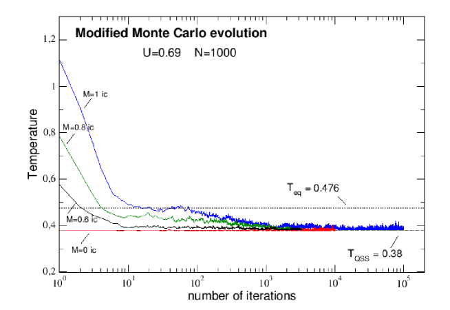
   Figure 4: We plot four examples of temperature evolution for the energy density $U=0.69$ and $N=1000$ obtained with the modified Monte Carlo procedure at constant energy. The curves refer to various initial conditions with uniform distribution of momenta and magnetization M=1,0.8,0.6,0, see text. We report also the values of temperature for the canonical equilibrium $T_{eq}=0.476$ and for the QSS regime in the infinite size limit $T_{QSS}=0.38$.

   The solutions of eq.(9) are

   $$\Theta=\pm arccos~{}R^{\pm}$$ (10)

   with

   $$R^{\pm}=\frac{ac\pm bD}{a^{2}+b^{2}},~{}~{}~{}-1\leq R^{\pm}\leq 1,~{}~{}~{}D^{2}=a^{2}+b^{2}-c^{2}\geq 0~{}.$$ (11)

   Thus, from eq.(10), one can calculate the new value of the $k$th angle, taking into account the new constraints (11). Then one can repeat the algorithm for the new configuration $C^{\prime}$ and so on, until the system reaches a stationary state. At this point, the desired expectation values (in this case the temperature of the system at fixed energy density) can be calculated by means of eq.(5).

3.2 Numerical results

With this new Monte Carlo algorithm, we calculated a new out-of equilibrium caloric curve for the HMF model, which corresponds to those states with minimal temperature at constant total energy density.
In our simulations we consider N=1000 rotators and different initial conditions with uniform distribution of momenta and different initial magnetization varying from $M=1$ to $M=0$ [8]. Then we follow the system evolution until a stationary value of temperature has been reached for each energy density value considered. In Fig.4 we show for example the temperature evolution in phase space for $U=0.69$. The plot shows that, using this new optimization algorithm, the Boltzmann-Gibbs equibrium temperature $T_{eq}=0.476$ is not a stable minimum, the curve for $M=1$ stays there for a while and then escapes to reach a deeper minimum. Instead, as expected for this energy density, the most stable solution is always the temperature corresponding to the homogeneous QSS $T_{QSS}=0.38$, also reported in the figure.

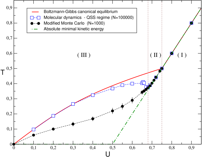
Figure 5: The caloric curve obtained with the Monte Carlo optimization procedure (full points) is compared with the Boltzmann-Gibbs canonical prediction at equilibrium (full curve) and with the metastable QSS caloric curve (open squares) obtained by means of the molecular dynamics microcanonical simulations in the QSS regime. We report for comparison also the curve corresponding to the a-priori absolute minimal values of kinetic energy (dot-dashed). We can distinguish three different regions: (I) In the homogeneous phase all the curves coincide. (II) In the energy interval $0.68\leq U\leq U_{c}$ ($U_{c}=0.75$) - marked by the two vertical dashed lines - the Monte Carlo curve differs from the Boltzman-Gibbs equilibrium prediction, and lies on the extension of the high temperature branch as the microcanonical dynamical simulations. (III) Below U=0.68, while the molecular dynamics curve rejoins again the canonical one, the Monte Carlo curve remains at a lower (but not at its absolute minimum) temperature value for the whole condensed phase.

In fig.5 we plot the caloric curve obtained with this new Monte Carlo optimization approach (full points). The bars reported indicate the size of the fluctuations. In comparison we show also the Boltzmann-Gibbs canonical equilibrium prediction (full line) and the metastable caloric curve found by means of molecular dynamics microcanonical simulations, performed for N=100000 with M1 initial conditions, in the QSS regime (open squares) [8]. It is helpful to divide the graph in three regions.
In region (I), i.e. in the homogeneous high temperature phase, the three curves coincide. This means that in this phase the Monte Carlo optimization method is able to recover the expected canonical equilibrium curve. This is in agreement with the fact that here the total energy is essentially kinetic: the potential energy is constant and equal to its maximum value V/N=0.5.
On the contrary, in region (II) - i.e. between $U_{c}$ and $U\sim 0.68$ - the Monte Carlo curve deviates from the canonical prediction, but coincides with the results of the molecular dynamics simulations in the QSS regime. As in the previous region, here also the Monte Carlo temperature takes its minimum allowed value, consistently with the total energy constraint. This fact is interesting in order to understand the nature of the QSS regime, which here corresponds to a stable attractor of the system when the magnetization (and the force acting on the single spin) is zero. We have checked that this result does not change with the number of spins considered.
Below the value $U=0.68$ - just lower than the value ($U=0.69$) where the QSS dynamical anomalies and the disagreement with the canonical prediction are more evident - the Monte Carlo curve starts to disagree also with the molecular dynamics simulations. In fact, in the region (III), while the QSS anomalies tend to disappear and the molecular dynamics curve slowly rejoins (below $U=0.5$) the canonical Boltzmann-Gibbs equilibrium prediction, the Monte Carlo curve stays below the other two curves. However the Monte Carlo result does not correspond to the absolute minimum value of temperature. In Fig.5 we report, for comparison, the curve (dot-dashed) corresponding to the a-priori absolute minimum value of kinetic energy. The Monte Carlo curve differs from such a minimal kinetic energy - which corresponds to $M=0$ - around the limiting value $U\sim 0.68$. This is a numerical confirmation of the instability of the homogeneous quasi-stationary states below this value as found in the nonlinear stability test of ref. [15].
Finally, it is interesting to observe that below the value $U=0.5$, where the kinetic energy - and therefore the temperature - could also be null, the Monte Carlo curve lies roughly in the middle between zero and the equilibrium temperature values. This result is not fully understood and could be originated by a competition between the two unstable attractors in phase space. Further investigations in this respect is required.

4 Conclusions

In this paper we have presented a Monte Carlo study of the HMF model. In the first part of the paper by means of a standard Metropolis procedure, we were able to reproduce the canonical caloric curve of the HMF model at equilibrium and study finite size effects close to the critical point where dynamical anomalies exist in the out-of-equilibrium regime. In the second part of the paper we studied out-of-equilibrium states by means of a Monte Carlo optimization technique. To this end, we have modified the standard Metropolis algorithm, in order to obtain a temperature minimization at constant energy density and look for those states with minimal temperature, which are not Boltzmann-Gibbs equilibrium states. However in this way we could study those metastable homogeneous Quasi Stationary States found dinamically below the phase transition point. We found that these states are stable for energy densities greater than $U\sim 0.68$. For energy densities smaller than this value, the zero magnetization quasi-stationary states are not reached and a different caloric curve is obtained. These results confirm what found in [15] by means of a nonlinear stability analysis where the authors suggest that this fact is due to the loose of stability of the spatially homogeneous solutions of Vlasov equation. We hope that this work, supplying a non-dynamical point of view and adding new numerical results to the study of the HMF model, will be of help in sheding further light on the nature of the several intriguing aspects of this model.

We thank C. Anteneodo, F. Baldovin, V. Latora and C. Tsallis for stimulating discussions. We would like to dedicate this paper to Constantino Tsallis for his 60th birthday wishing him a still very long and fruitful research activity.

References

- [1] M. Antoni and S.Ruffo, Phys. Rev. E 52 (1995) 2361.
- [2] For a recent review on this model see also: T. Dauxois, V. Latora, A. Rapisarda, S. Ruffo, A. Torcini, in Dynamics and Thermodynamics of Systems with Long-Range Interactions T. Dauxois, S. Ruffo, E. Arimondo, M. Wilkens Eds., Lecture Notes in Physics Vol. 602, Spinger (2002) p.458 and references therein.
- [3] V. Latora , A. Rapisarda and C. Tsallis, Phys. Rev. E 64 (2001) 056134.
- [4] A. Pluchino, V. Latora, A. Rapisarda, Continuum Mechanics and Thermodynamics 16 (2004) 245.
- [5] C. Tsallis, A. Rapisarda, V. Latora, F. Baldovin in Dynamics and Thermodynamics of Systems with Long-Range Interactions T. Dauxois, S. Ruffo, E. Arimondo, M. Wilkens Eds., Lecture Notes in Physics Vol. 602, Spinger (2002), p.140 and references therein.
- [6] Nonextensive Entropy: interdisciplinar ideas, C. Tsallis and M. Gell-Mann Eds., Oxford University Press (2004).
- [7] A. Cho, Science 297 (2002) 1268; Letters to the Editors by S. Abe, A.K. Rajagopal; A. Plastino; and V. Latora, A. Rapisarda, A. Robledo, Science 300 (2003) 249.
- [8] A. Pluchino, V. Latora, A. Rapisarda, Physica D 193 (2004) 315.
- [9] M.A.Montemurro, F.A.Tamarit and C.Anteneodo, Phys. Rev. E 67 (2003) 031106.
- [10] A. Pluchino, V. Latora, A. Rapisarda, Phys. Rev. E 69 (2004) 056113.
- [11] A. Pluchino, V. Latora, A. Rapisarda, Physica A 340 (2004) 187.
- [12] D.H.E. Gross, Microcanonical Thermodynamics: phase transitions in small systems, Lecture Notes in physics, vol.66, World Scientific, Singapore 2001, pg.196-197.
- [13] R. Salazar, R. Toral, A.R. Plastino, Physica A 305 (2002) 144.
- [14] D.P. Landau and K. Binder, A Guide to Monte Carlo Simulations in Statistical Physics Cambridge University Press (2000).
- [15] C.Anteneodo and Raul O.Vallejos, Physica A (2004) in press [cond-mat/0401195].
- [16] Y. Yamaguchi, J.Barré, F.Bouchet, T.Dauxois and S.Ruffo, Physica A 337 (2004) 653.