Instanton calculus for the self-avoiding manifold model

Abstract

We compute the normalisation factor for the large order asymptotics of perturbation theory for the self-avoiding manifold (SAM) model describing flexible tethered ($D$-dimensional) membranes in $d$-dimensional space, and the $\epsilon$-expansion for this problem. For that purpose, we develop the methods inspired from instanton calculus, that we introduced in a previous publication (Nucl. Phys. B 534 (1998) 555), and we compute the functional determinant of the fluctuations around the instanton configuration. This determinant has UV divergences and we show that the renormalized action used to make perturbation theory finite also renders the contribution of the instanton UV-finite. To compute this determinant, we develop a systematic large-$d$ expansion. For the renormalized theory, we point out problems in the interplay between the limits $\epsilon\to 0$ and $d\to\infty$, as well as IR divergences when $\epsilon=0$. We show that many cancellations between IR divergences occur, and argue that the remaining IR-singular term is associated to amenable non-analytic contributions in the large-$d$ limit when $\epsilon=0$. The consistency with the standard instanton-calculus results for the self-avoiding walk is checked for $D=1$.

Saclay Preprint T04/122  

I Introduction

Flexible polymerized 2-dimensional films (tethered or polymerized membranes) NelPel87 have very interesting statistical properties (for a review see Jerusalem87 , Jerusalem87-II , Wiesehabil ). In these objects there is a competition between entropy which favors crumpled or folded configurations as for polymers, steric interactions (self-avoidance) which tend to swell the membranes, and bending rigidity which favors flat configurations. Internal disorder, inhomogeneities and anisotropy may also play an important role, that we shall not discuss here (see the chapters 10-12 in Jerusalem87-II and Wiesehabil for a recent review of these effects).

If one does not take into account self-avoidance, theoretical arguments (mean-field and renormalization-group calculations) and numerical simulations show two phases: (1) A high-temperature/low-rigidity crumpled phase, where the membrane is crumpled with infinite Hausdorff dimension, and where bending rigidity is irrelevant; (2) a low-temperature (flat) phase with large effective rigidity and Hausdorff dimension two KanKarNel86 , KanKarNel87 .

In the high-temperature (crumpled) phase, steric interactions (self-avoidance) are physically relevant, and will swell the membrane, as for polymers. Two scenarios are possible: Either the membrane is flat with Hausdorff dimension two (as for high bending rigidity), or it is crumpled swollen with Hausdorff dimension larger than two. For large imbedding dimension $d$ a Gaussian variational approximation can be argued to become exact, predicting a Haussdorff dimension $d_{\mathrm{H}}=d/2$. It is non-trivial whether this swollen phase exists down to $d=3$. Numerical simulations indicate that only a flat phase exists in $d=3$; for details see the discussion in Jerusalem87-II , Wiesehabil . However, simulations are for rather small systems. It therefore remains important to have a solid theoretical understanding.

The theory in question is a generalization of the Edwards model for polymers Edw65 , CloJan90 . It was proposed in AroLub88 , KarNel87 , KarNel88 , and is a model of self-avoiding manifolds (or membranes), hereafter denoted the SAM model. It is amenable to a treatment by perturbation theory (in the coupling constant of steric interactions) and to a perturbative renormalization group analysis which leads to a Wilson-Fisher like $\epsilon$-expansion for estimating the scaling exponents and the critical properties of the swollen phase.

This SAM model is quite interesting at the theoretical level for several reasons:

1. It can only be defined as a non-local field-theory over the internal 2-dimensional space of the manifold, with infinite-ranged multi-local interactions. Therefore the applicability of renormalization theory and of renormalization group techniques is a non-trivial issue. A proof of perturbative renormalizability to all orders was finally given in DDG3 , GBU .

2. The model is in fact defined through a double dimensional continuation, where both the dimension of space $d$ and the internal dimension $D$ of the manifold are analytically continued to non-integer values. The physical case of two-dimensional membranes is always in the strong-coupling regime where the engineering dimension of the coupling, $\epsilon=2D-\frac{2-D}{2}d$ is $\epsilon=4$ for any space dimension $d$.

3. The analytical study of this model at the non-perturbative level is still in its infancy, since it is a technically quite difficult problem. A first step was made by the two present authors for the large orders of perturbation theory in DavidWiese1998 . It is this issue of the large-order asymptotics of the SAM model that we treat in this paper.

For quantum mechanics Dyson52 , Lam68 , BenderWu69 and for local quantum field theories Lip76 (such as the Laudau-Ginzburg-Wilson $\phi^{4}$ theories) the large-order asymptotics of perturbation theory are known to be controlled by (in general complex) finite-action solutions of the classical equation of motion called “instantons”. More precisely the large-order asymptotics are described by semi-classical approximations around these instantons. We refer for instance to Zin82 for a review of this “instanton calculus”.

In DavidWiese1998 we have shown that similarly for the SAM model there exists an instanton which controls its large-order asymptotics. This instanton is a scalar field configuration in the external $d$-dimensional space, which extremizes a highly non-local effective-action functional, and which cannot be computed exactly. We also showed that remarkable simplifications occur in the large-$d$ limit, which suggests that a systematic $1/d$ expansion can be constructed to study the instanton, but also that already the first $1/d$ correction to the large-$d$ limit is plagued with infrared (IR) divergences whose origin was unclear. In DavidWiese1998 we only studied the instanton at the classical level, i.e. the (non-local) equation of motion and the properties of its solution, the instanton.

In this article we present the full semi-classical analysis of the instanton for the SAM model, derive its connection with the large-order asymptotics, and study the UV divergences and renormalization necessary for the instanton. For this purpose, many new calculational techniques had to be developed, hence the length of the paper and its technical character. More precisely, the main new results are:

1. We first show in much more details than in DavidWiese1998 how the instanton emerges from the functional integral which defines the continuum SAM model. In particular we treat properly and carefully the zero-modes for the instanton, how the contour of functional integration has to be deformed in the complex saddle-point method, as well as various normalization problems for the functional integration. This is done in Sect. III-A,B.

2. Using this, we obtain the contribution of the fluctuations around the instanton in the semi-classical approximation as the determinant of a non-local kernel operator in $d$-dimensional space, and derive the normalization factor for the large-order asymptotics (Sect. III-C,D,E).

3. We analyze completely the UV divergences of this determinant, and show that in the renormalized theory these UV divergences for the instanton determinant factor are canceled by the one-loop perturbative counterterm of the renormalized theory, making the final asymptotics UV finite. This is an important check of the consistency of the SAM model, since the original proof of renormalizability is only valid in perturbation theory. (In a field theoretic language it is not a background-independent proof). This is done in Sect. IV. Our argument is based on the extension of the perturbative renormalizability argument to the general case of ensembles of interacting manifolds in an external background potential.

4. In DavidWiese1998 the instanton equation was solved within a variational approximation. In sect. V we study how this approximation can be applied to the explicit calculation of the instanton determinant factor. We first show that a direct variational calculation gives a result which is too naive, and does not take properly into account the UV fluctuations. We then propose a systematic framework to construct an expansion around the variational approximation, developing ideas that we proposed in DavidWiese1998 . We then show that this framework gives the leading term for the instanton determinant factor in the large-$d$ limit.

5. We are thus able to construct a systematic $1/d$ expansion for the instanton calculus, and show that this expansion is well defined as long as the SAM is super renormalizable, i.e. $\epsilon>0$ (no UV divergences in perturbation theory, apart from vacuum energy terms). The leading and first subleading terms are computed explicitly for the determinant factor and the normalization factor of the zero mode of the instanton. These calculations involve a new non-trivial diagrammatic expansion. This is done in Sect. VI .

6. Finally we study the $1/d$ expansion for the renormalized theory at $\epsilon=0$. We show that, at variance with the instanton calculus for local field theories, some subtle issues arise for the SAM model. Indeed, we show that already at leading order in $d$, the limits $d\to\infty$ and $\epsilon\to 0$ do not commute, and that some care is needed in order to obtain the instanton determinant factor for the renormalized theory at large $d$. We then show that the subleading terms of the $1/d$ expansion are plagued with IR divergences at $\epsilon=0$, generalizing the results of DavidWiese1998 . We analyze completely these IR divergences at the first subleading order, and show that many compensations occur, leaving a single IR-singular term associated with a single eigenmode for the fluctuations around the instanton, namely the unstable eigenmode generated by global dilation for the instanton. This analysis of the renormalized theory is done in Sect. VII.

To summarize, we have performed a non-trivial check of the consistency of the model, in particular of its renormalization, in a non-perturbative regime, and we have developed the tools to compute the large-order asymptotics of the SAM model.

Appendices contain more technical computations and details about the normalizations. In particular in appendix C we explicitly check that in the special case of the self-avoiding polymer ($D=1$) we recover the large-order asymptotics of the Edwards model obtained by field theoretical methods (using instanton calculus and the well known equivalence between the Edwards model and the O($n=0$) $\phi^{4}$ Landau Ginzburg model Gen72 , Clo81 ). This provides a check of the consistency of the SAM model.

II The model

II.1 The non-interacting manifold

First we define the model for the Gaussian non-interacting manifold (free or phantom manifold). Of course this model reduces to a massless free field, but we reconsider it closely in order to fix properly the normalization for the measure and for the definition of the observables, and for the treatment of the zero modes.

II.1.1 The model and its action

We consider a manifold $\mathcal{M}$ with a finite size, as a closed $D$-dimensional manifold $\mathcal{M}$, with a fixed internal (or intrinsic) Riemannian structure, given by a metric tensor $\mathsf{g}=g_{\mu\nu}(\mathsf{x})$. $\mathsf{x}=(x^{\mu};\ \mu=1,\ldots,D$) describes (a system of) local coordinates on $\mathcal{M}$. From now on the internal volume of $\mathcal{M}$, $\mathrm{Vol}(\mathcal{M})$ and its internal size $L$ are defined as

$$\mathrm{Vol}(\mathcal{M})\ =\ \int_{\mathcal{M}}\mathrm{d}^{D}\mathsf{x}\,\sqrt{g}\quad,\quad L\ =\ \mathrm{Vol}(\mathcal{M})^{{\frac{1}{D}}}$$ (1)

with $g=\det[\mathsf{g}]$. The manifold is embedded in external (or bulk) $d$-dimensional Euclidean space $\mathbb{R}^{d}$. This embedding is described by the field $\mathsf{r}=\{r^{a};\ a=1,\ldots,d\}$

$$\mathcal{M}\to\mathbb{R}^{d}\ \ ,\ \ \mathsf{x}\to\mathsf{r}(\mathsf{x})$$ (2)

We shall use dimensional regularization in this paper by considering that the internal dimension $D$ of the manifold is $0<D<2$ non-integer. See the reference paper GBU for a more precise discussion of how we can define a finite membrane within dimensional regularization. In practice we can restrict ourselves to the case of a square $D$-dimensional torus of size $L$, $\mathbb{T}_{D}=\left(\mathbb{R}^{D}/(L\cdot\mathbb{Z})^{D}\right)$, with flat metric $g_{\mu\nu}=\delta_{\mu\nu}$.

We first consider the free non-interacting manifold (phantom membrane). The manifold may fluctuate freely in external $d$-dimensional space. Its free energy is given by the Gaussian local elastic term $S_{0}$, which is the integral of the square of the gradient of the field $\mathsf{r}$

$$S_{0}[\mathsf{r}]\ =\ \int_{\mathcal{M}}{1\over 2}(\nabla\mathsf{r})^{2}\ =\ \int\mathrm{d}^{D}\mathsf{x}\,\sqrt{g}\,{1\over 2}g^{\mu\nu}\partial_{\mu}\mathsf{r}\cdot\partial_{\nu}\mathsf{r}\ .$$ (3)

This is nothing but the Euclidean action for a free massless field (with $d$ components) living on $\mathcal{M}$. The manifold may (and does) freely intersect itself, as does a random Brownian walk in $d\leq 4$ space dimensions.

II.1.2 The partition function

The partition function for the free manifold is thus given by the functional integral

$$Z_{0}\ =\ \int\mathcal{D}[\mathsf{r}]\,\mathrm{e}^{-S_{0}[\mathsf{r}]}$$ (4)

where $\mathcal{D}[\mathsf{r}]$ is the standard functional measure for the free massless field $\mathsf{r}$ (see Appendix A for details and the normalization used in this paper).

There is an infinite factor in $Z_{0}$ (the volume of bulk space Vol($\mathbb{R}^{d}$)) coming from the translational zero mode of the manifold. This can be isolated by choosing a specific point $\mathsf{x}_{0}$ on the manifold and a specific point $\mathsf{r}_{0}$ in bulk space, and by defining the partition function $\mathcal{Z}_{0}$ for a marked manifold

$$\mathcal{Z}_{0}\ =\ \mathcal{Z}_{0}(\mathsf{r}_{0})\ =\ \int\mathcal{D}[\mathsf{r}]\,\delta^{d}(\mathsf{r}(\mathsf{x}_{0})-\mathsf{r}_{0})\,\mathrm{e}^{-S_{0}[\mathsf{r}]}$$ (5)

$\mathcal{Z}_{0}(\mathsf{r}_{0})$ is infra-red (IR) finite and does not depend on the choice of $\mathsf{r}_{0}$ or of $\mathsf{x}_{0}$. We have formally

$$\qquad Z_{0}\ =\ \int\mathrm{d}^{d}\mathsf{r}_{0}\ \mathcal{Z}_{0}(\mathsf{r}_{0})\ =\ \mathrm{Vol}(\mathbb{R}^{d})\,\mathcal{Z}_{0}\ .$$ (6)

The partition function $\mathcal{Z}_{0}$ is found to be related to the determinant of the Laplacian operator over $\mathcal{M}$ through

$$\mathcal{Z}_{0}(\mathsf{r}_{0})\ =\ \Big{[}{\det}^{\prime}\left[-\Delta\right]\cdot 2\pi/\mathrm{Vol}(\mathcal{M})\Big{]}^{-d/2}\ ,$$ (7)

where ${\det}^{\prime}\left[-\Delta\right]$ is the product of the non-zero eigenvalues of (minus) the Laplacian operator $\Delta=g^{-1/2}\partial_{\mu}g^{\mu\nu}\partial_{\nu}$ on $\mathcal{M}$. $\mathrm{Vol}(\mathcal{M})=\int\mathrm{d}^{D}\mathsf{x}\,\sqrt{g}$ is the internal volume of the manifold. This last term comes from the proper treatment of the translational zero mode of the Laplacian (see Appendix A).

The determinant ${\det}^{\prime}\left[-\Delta\right]$ is ultra-violet (UV) divergent, and is defined through a zeta-function regularization (for a manifold $\mathcal{M}$ with non-integer dimension $D\neq 1$ or $2$ this is equivalent to dimensional regularization)

$$\log({\det}^{\prime}\left[-\Delta\right])\ =\ -\zeta^{\prime}(0)\quad,\quad\zeta(s)=\mathrm{tr}^{\prime}(\left(-\Delta\right)^{-s})\ .$$ (8)

The zeta-function $\zeta(s)$ is defined by analytic continuation from $\mathrm{Re}(s)$ large. $\mathrm{tr}^{\prime}$ means the trace over the space orthogonal to the kernel of $\Delta$. $\zeta(s)$, scales with the size of $\mathcal{M}$ as

$$\zeta(s)\ =\ \left[\mathrm{Vol}(\mathcal{M})\right]^{2s/D}\,\tilde{\zeta}(s)\ ,$$ (9)

where the “normalized zeta-function” $\tilde{\zeta}(s)$ depends on the shape of the manifold but not on its size (scale invariance). In the absence of a conformal anomaly, as this is the case for the generic case of $D$ non-integer we have the exact identity

$$\zeta(0)\ =\ -1\ .$$ (10)

(This factor comes from the contribution of the subtracted zero mode in the determinant). Hence the partition function reads

$$\mathcal{Z}_{0}(\mathsf{r}_{0})\ =\ \left[\mathrm{Vol}(\mathcal{M})\right]^{-{d(2-D)\over 2D}}\,\left[{\mathrm{e}^{\tilde{\zeta}^{\prime}(0)}\over 2\pi}\right]^{d/2}\ .$$ (11)

The last term is a “form factor” depending on the shape of $\mathcal{M}$.

For 2-dimensional manifolds ($D=2$), the conformal anomaly gives an additional scale factor of the form ${|L\mu_{0}|}^{\chi\,d/6}$, where $L=\mathrm{Vol}(\mathcal{M})^{1/D}$ is the size of $\mathcal{M}$, $\mu_{0}$ the regularization mass scale, required to define properly the measure in the functional integral (see Appendix A), and $\chi$ the Euler characteristics of the membrane. We shall not discuss this any further, since this is not relevant for the problem treated here, where we consider manifolds with $D<2$.

II.2 The interacting self-avoiding manifold

II.2.1 The action

The steric self-avoiding interaction is introduced by adding a 2-body repulsive contact interaction term of the form

$$\int_{\mathsf{x}}\int_{\mathsf{y}}\delta^{d}(\mathsf{r}(\mathsf{x})-\mathsf{r}(\mathsf{y})\ =\ \int_{\mathcal{M}}\mathrm{d}^{D}\mathsf{x}\sqrt{g(x)}\,\int_{\mathcal{M}}\mathrm{d}^{D}\mathsf{y}\sqrt{g(x)}\,\delta^{d}(\mathsf{r}(\mathsf{x})-\mathsf{r}(\mathsf{y}))$$

(where $\delta^{d}(\mathsf{r})$ is the Dirac distribution in the external space $\mathbb{R}^{d}$ ) to the action, which is now

$$S[\mathsf{r},b]=\ \int_{\mathcal{M}}{1\over 2}(\nabla\mathsf{r})^{2}\ +\ {b\over 2}\int_{\mathsf{x}}\int_{\mathsf{y}}\delta^{d}(\mathsf{r}(\mathsf{x})-\mathsf{r}(\mathsf{y}))$$ (12)

$b>0$ is the self-avoidance coupling constant. This is similar to what is done in the Edwards model for polymers.

II.2.2 The partition functions

The partition function for the self-avoiding manifold is

$$\mathcal{Z}(\mathsf{r}_{0},b)=\ \int\mathcal{D}[\mathsf{r}]\,\delta^{d}(\mathsf{r}(\mathsf{x}_{0})-\mathsf{r}_{0})\,\mathrm{e}^{-S[\mathsf{r},b]}\qquad;\qquad Z(b)\ =\ \int\mathrm{d}^{d}\mathsf{r}_{0}\,\mathcal{Z}(\mathsf{r}_{0},b)\ .$$ (13)

These partition functions are defined in perturbation theory, within a dimensional regularization scheme, i.e. by analytic continuation in the internal dimension $D$.

If the internal coordinate $\mathsf{x}$ has engineering dimension $1$, the external coordinate $\mathsf{r}$ has engineering dimension $\nu_{0}$ given by (i.e. $[\mathsf{r}]\sim[\mathsf{x}]^{\nu_{0}}$)

$$\nu_{0}\ =\ (2-D)/2$$ (14)

and the coupling constant $b$ has engineering dimension $-\epsilon$ (i.e. $[b]\sim[\mathsf{x}]^{-\epsilon}$) with

$$\epsilon\ =\ 2D-(2-D)d/2$$ (15)

As usual in polymer and membrane problems, we shall consider mainly the normalized partition function $\mathfrak{Z}(b)$, defined by the ratio of the interacting partition function for the interacting manifold $\mathcal{M}$, divided by the partition function for the same manifold $\mathcal{M}$, but free.

$$\mathfrak{Z}(b)\ =\ Z(b)/Z_{0}\ =\ \mathcal{Z}(\mathsf{r}_{0},b)/\mathcal{Z}_{0}(\mathsf{r}_{0})\ .$$ (16)

Let

$$L\ =\ (\mathrm{Vol}(\mathcal{M}))^{1/D}\quad;\qquad\mathrm{Vol}(\mathcal{M})\,=\,\int_{\mathcal{M}}\mathrm{d}^{D}\mathsf{x}\,\sqrt{g(\mathsf{x})}$$ (17)

be the internal size of the manifold. The normalized partition function has a perturbative series expansion in powers of $b$, of the form

$$\mathfrak{Z}(b)\ =\ 1\,+\,\sum_{k=1}^{\infty}\mathfrak{Z}_{k}\,\left(bL^{\epsilon}\right)^{k}$$ (18)

where the coefficients $\mathfrak{Z}_{k}$ depend only on the shape of the manifold, on its internal dimension $D$, and on the external dimension $d$. These coefficients are given by the expectation value in the massless free theory defined by the free action $S_{0}$ of the bi-local operators corresponding to the interaction term

$$\mathfrak{Z}_{k}\ =\ {1\over k!\,2^{k}}\,\iint_{\mathsf{x}_{1},\mathsf{y}_{1}}\cdots\iint_{\mathsf{x}_{k},\mathsf{y}_{k}}\ \big{\langle}\prod_{i=1,k}\delta^{d}(\mathsf{r}(x_{i})-\mathsf{r}(y_{i}))\big{\rangle}_{0}\ ,$$ (19)

with $\langle\dots\rangle_{0}$ the expectation value w.r.t. ${\cal S}_{0}[r]$, see (3).

II.2.3 Observables and correlation functions in external space

We shall be mainly interested in correlations functions which correspond to observables which are global for the manifold (i.e. do not depend on the internal position of specific points on the manifold), but which may be local in external space (i.e. do depend on the position of specific points in the external space). These observables are the simplest ones. In particular for the case $D=1$ (polymers) these observables have a direct interpretation in terms of correlation functions of local operators in the corresponding local field theory in external $d$-dimensional space.

The observables involve the manifold density $\rho(\mathsf{r})$. We define the manifold density at the point $\mathsf{r}_{1}$, $\rho(\mathsf{r}_{1})$, as the functional of the field $\mathsf{r}(x)$

$$\rho(\mathsf{r}_{1};\mathsf{r})\ =\ \int_{\mathsf{x}}\delta^{d}(\mathsf{r}(\mathsf{x})-\mathsf{r}_{1})\ .$$ (20)

The $N$-point density correlator $\mathcal{R}^{(N)}(\mathsf{r}_{1}\cdots\mathsf{r}_{N})$ for the interacting manifold is defined as

$$\mathcal{R}^{(N)}(\mathsf{r}_{1}\cdots\mathsf{r}_{N};b)\ =\ \int\mathcal{D}[\mathsf{r}]\,\prod_{i=1}^{N}\,\rho(\mathsf{r}_{i};\mathsf{r})\,\mathrm{e}^{-S(\mathsf{r},b)}\ .$$ (21)

Obviously the one-point density correlator is related to the partition function (for a one-point marked manifold) by

$$\mathcal{R}^{(1)}(\mathsf{r}_{0};b)\ =\ \mathrm{Vol}(\mathcal{M})\,\mathcal{Z}(\mathsf{r}_{0};b)\ .$$ (22)

Ratios of density correlators define expectation values of densities. For instance, the e.v. (expectation value) of a product of $N$ density operators $\rho(\mathsf{r}_{i})$ for a manifold constrained to be attached to a point $\mathsf{r}_{0}$ is the ratio

$$\langle\rho(\mathsf{r}_{1})\cdots\rho(\mathsf{r}_{N})\rangle_{\mathsf{r}_{0};b}\ =\ \mathcal{R}^{(N+1)}(\mathsf{r}_{0},\mathsf{r}_{1}\cdots\mathsf{r}_{N};b)/\mathcal{R}^{(1)}(\mathsf{r}_{0};b)\ .$$ (23)

As for the partition functions, it is more convenient to normalize the density correlators with respect to the partition function for the free manifold. We thus define the normalization for the normalized density correlators, by

$$\mathfrak{R}^{(N)}(\mathsf{r}_{1}\cdots\mathsf{r}_{N};b)\ =\ \mathcal{R}^{(N)}(\mathsf{r}_{1}\cdots\mathsf{r}_{N};b){\Bigg{/}}\mathrm{Vol}(\mathcal{M})\,\mathcal{Z}_{0}\ .$$ (24)

In particular the normalized 1-point correlator coincides with the normalized partition function

$$\mathfrak{R}^{(1)}(\mathsf{r}_{1};b)\ =\ \mathfrak{Z}(b)$$ (25)

and is independent of $\mathsf{r}_{1}$.

These observables have a perturbative series expansion in the coupling constant $b$. In particular they scale with the size $L$ of the manifold as

$$\mathcal{R}^{(N)}(\mathsf{r}_{1}\cdots\mathsf{r}_{N};b,L)\ =\ L^{N(\epsilon-D)}\cdot\mathcal{R}^{(N)}(\mathsf{r}_{1}\,L^{-\nu_{0}},\cdots,\mathsf{r}_{N}\,L^{-\nu_{0}};bL^{\epsilon})$$ (26)

and

$$\mathfrak{R}^{(N)}(\mathsf{r}_{1}\cdots\mathsf{r}_{N};b,L)\ =\ L^{(N-1)(\epsilon-D)}\cdot\mathfrak{R}^{(N)}(\mathsf{r}_{1}\,L^{-\nu_{0}},\cdots,\mathsf{r}_{N}\,L^{-\nu_{0}};bL^{\epsilon})$$ (27)

II.2.4 Global quantities and gyration radius moments

We define the moments of order $k$ for the gyration radius (in short the $k$-th gyration moment) $\mathsf{R_{gyr}^{(k)}}$ of the manifold by

$$\mathsf{R_{gyr}^{(k)}}={\int_{\mathsf{x}_{1}}\int_{\mathsf{x}_{2}}\left|\mathsf{r}(\mathsf{x}_{1})-\mathsf{r}(\mathsf{x}_{2})\right|^{k}\over\int_{\mathsf{x}_{1}}\int_{\mathsf{x}_{2}}1}\ .$$ (28)

The standard gyration radius is $\mathsf{R}_{\mathrm{gyr}}=\sqrt{\mathsf{R_{gyr}^{(2)}}}$. The expectation value $\mathcal{R}_{\mathrm{gyr}}^{(k)}$ of the $k$-th gyration moment $\mathsf{R_{gyr}^{(k)}}$ for the interacting manifold is thus (for $k>0$)

$$\mathcal{R}_{\mathrm{gyr}}^{(k)}\ =\ \langle\mathsf{R_{gyr}^{(k)}}\rangle\ =\ {1\over\mathrm{Vol}(\mathcal{M})^{2}}\,\int_{\mathsf{r}_{1}}\int_{\mathsf{r}_{2}}\left|\mathsf{r}_{1}-\mathsf{r}_{2}\right|^{k}\,\mathcal{R}^{(2)}(\mathsf{r}_{1},\mathsf{r}_{2};b)\ .$$ (29)

II.3 UV divergences and perturbative renormalization

Using dimensional regularization, the perturbative expansion for the partition function and the observables is known to be UV finite for

$$0<D<2\quad\text{and}\quad D<\epsilon\qquad\text{i.e.}\qquad d<{2D\over 2-D}\ .$$ (30)

As long as we deal with finite-size manifolds ($L<\infty$), perturbation theory is free from infra-red divergences (which occur for infinite manifolds since perturbation theory is made around the free-manifold theory, which is a free massless scalar field in $D\leq 2$ dimensions).

The perturbative expansion suffers from short-distance (UV) divergences when

$$D\,\leq\,\epsilon\ .$$ (31)

These UV divergences come from the short-distance behavior of the expectation values which appear as integrands in the integrals, when the distance between several points $\mathsf{x}_{i}$ and $\mathsf{y}_{j}$ goes to zero. Using dimensional regularization these divergences appear as poles in $\epsilon$ ($d$ being fixed), or equivalently as lines of singularity in the $(d,D)$ plane.

As proved in GBU , these UV divergences can be studied within a multi-local operator product expansion (MOPE) which generalizes Wilson’s OPE of local field theory. As a consequence, these UV divergences are proportional to the insertion of multi-local operators, and are amenable to renormalization theory.

The MOPE formalism and dimensional analysis show that for $0<\epsilon\leq D$ there is a finite number of divergences, with poles at

$$\epsilon\ =\ D/n\ ,\ n\in\mathbb{N_{+}}\ .$$ (32)

These divergences are proportional to insertions of the identity operator $\mathbf{1}$ (with dimension $0$). The model is super-renormalizable for $\epsilon>0$ and these divergences are subtracted by adding to the action a local counterterm proportional to the volume of the manifold (i.e. to the integral of the identity operator $\mathbf{1}$).

$$\Delta S(\mathsf{r})\ \propto\ \int_{\mathsf{x}}\mathbf{1}\ =\ \mathrm{Vol}(\mathcal{M})\ \ .$$ (33)

These divergences and the corresponding counterterm are constant terms, independent of the configuration of the manifold, i.e. of the field $\mathsf{r}$, and they disappear in the observables given by ratios of correlators such as the e.v. $\langle\rho(\mathsf{r}_{1})\cdots\rho(\mathsf{r}_{N})\rangle_{\mathsf{r}_{0}}$ and the normalized correlators $\mathfrak{R}^{(N)}$.

For $\epsilon=0$ the model has an infinite number of divergences. These divergences are proportional to the insertion of the two operators present in the original action $S$. This means that the theory is renormalizable, and that it can be made UV-finite by adding to the action counterterms of the same form than those of the original action. In other words, one can construct in perturbation theory a renormalized action

$$S_{\mathrm{r}}(\mathsf{r};b_{\mathrm{r}},\mu)\ =\ {Z(b_{\mathrm{r}})\over 2}\int_{\mathsf{x}}\left(\nabla\mathsf{r}\right)^{2}\,+\,{b_{\mathrm{r}}\mu^{\epsilon}Z_{b}(b_{\mathrm{r}})\over 2}\int_{\mathsf{x}}\int_{\mathsf{y}}\delta^{d}(\mathsf{r}(\mathsf{x})-\mathsf{r}(\mathsf{y}))\ ,$$ (34)

where $b_{\mathrm{r}}$ is the dimensionless renormalized coupling constant, $Z(b_{\mathrm{r}})$ and $Z_{b}(b_{\mathrm{r}})$ the wave-function and the coupling-constant renormalization factors, and $\mu$ is the renormalization momentum scale, while $\mathsf{r}(\mathsf{x})$ is now the renormalized field. This renormalized action is such that the renormalized correlation functions

$$\mathcal{R}_{r}^{(N)}(\mathsf{r}_{1}\cdots\mathsf{r}_{N};b_{\mathrm{r}},\mu)\ =\ \int\mathcal{D}[\mathsf{r}]\ \prod_{i=1}^{N}\rho(\mathsf{r}_{i};\mathsf{r})\,\mathrm{e}^{-S_{r}(\mathsf{r};b_{\mathrm{r}},\mu)}$$ (35)

have a perturbative series expansion in $b_{\mathrm{r}}$ which is UV finite for $\epsilon\geq 0$ and stays finite for $\epsilon=0$. For a finite manifold with size $L$ the renormalized perturbation theory is still IR finite.

From the standard arguments of renormalization group (RG) theory the renormalized theory describes the universal large-distance scaling behavior of self-avoiding manifolds. One can write RG equations which tell how the observables scale with the size of the manifold for $\epsilon>0$. When expressed in terms of the renormalized observables and the renormalized coupling, these RG equations have a regular limit (at least in perturbation theory) as $\epsilon\to 0_{+}$. As a consequence one can construct an $\epsilon$-expansion à la Wilson-Fisher for the scaling exponents.

II.4 Effective non-local model in external space

As shown in DavidWiese1998 , to study the large-order behavior of the SAM model as well as its large-$d$ behavior, it is necessary to reformulate the model as an effective non-local model for an auxiliary composite field $V(\mathsf{r})$ in the external $d$-dimensional space.We recall this reformulation.

II.4.1 Auxiliary fields and effective action

First we recall the auxiliary field $\rho(\mathsf{r})$ (local manifold density) defined in (20),

$$\rho({\mathsf{r}})=\int_{\mathsf{x}\in\mathcal{M}}\delta^{d}(\mathsf{r}(\mathsf{x})-\mathsf{r})$$ (36)

and its conjugate field $V(\mathsf{r})$, which is the Lagrange multiplier for the above constraint, such that

$$1\ =\ \int\mathcal{D}[V]\,\mathcal{D}[\rho]\,\exp\left({\int\mathrm{d}^{d}\mathsf{r}\,V(\mathsf{r})\left[\rho(\mathsf{r})-\int_{\mathcal{M}}\delta^{d}(\mathsf{r}(\mathsf{x})-\mathsf{r})\right]}\right)\ .$$ (37)

$\rho$ is a real field, while $V$ is imaginary, and has to be integrated from $-\mathrm{i}\infty$ to $+\mathrm{i}\infty$ in the functional integral. Equivalently the functional measures for $\rho$ and $V$ are formally

$$\int\mathcal{D}[\rho]\ =\ \int_{0}^{\infty}\prod_{\mathsf{r}}\mathrm{d}\rho(\mathsf{r})\ \equiv\ \int_{-\infty}^{\infty}\prod_{\mathsf{r}}\mathrm{d}\rho(\mathsf{r})\qquad;\qquad\int\mathcal{D}[V]\ =\ \int_{-\mathrm{i}\infty}^{\mathrm{i}\infty}\prod_{\mathsf{r}}{\mathrm{d}V(r)\over 2\mathrm{i}\pi}\ .$$ (38)

We now insert (37) in the functional integral. Since the interaction term can be written as

$$\int_{\mathsf{x}}\int_{\mathsf{y}}\delta^{d}(\mathsf{r}(\mathsf{x})-\mathsf{r}(\mathsf{y}))\ =\ \int_{\mathsf{r}}\rho(\mathsf{r})^{2}\ ,$$ (39)

the integral over the field $\rho$ is Gaussian and can be performed explicitly. We obtain for the partition function

$$Z(b)=\int\mathcal{D}[\mathsf{r}]\,\mathcal{D}[V]\,\exp\left[-\int_{\mathsf{x}}\left(\frac{1}{2}(\nabla_{\!\mathsf{x}}\mathsf{r})^{2}+V(\mathsf{r})\right)\,+\,{1\over 2b}\int_{\mathsf{r}}V(\mathsf{r})^{2}\right]\ .$$ (40)

Note that the functional measure $\mathcal{D}[V]$ over $V[\mathsf{r}]$ is now normalized so that

$$\int\mathcal{D}[V]\,\exp\left({1\over 2b}\int_{\mathsf{r}}V(\mathsf{r})^{2}\right)\ =\ 1\$$ (41)

and depends explicitly on the coupling constant $b$.

This functional integral describes a free (not self-interacting) manifold fluctuating in a random annealed potential $V(\mathsf{r})$. This is a simple generalization of the reformulation of the SAW problem into a random walk in a random annealed potential.

Now we integrate over the field $\mathsf{r}(\mathsf{x})$ and define the effective free energy $F_{\mathcal{M}}[V]$ for the non-interacting (phantom) manifold $\mathcal{M}$ in the external potential $V(\mathsf{r})$ by

$$\exp\left(-\,F_{\mathcal{M}}[V]\right)\ =\ \int\mathcal{D}[\mathsf{r}]\,\exp\left[-\int_{\mathsf{x}}\left(\frac{1}{2}(\nabla_{\!\mathsf{x}}\mathsf{r})^{2}+V(\mathsf{r})\right)\right]\ .$$ (42)

We are left with the effective action for the field $V$, $S_{\mathcal{M}}[V]$, which is given by

$$S_{\mathcal{M}}[V]\ =\ F_{\mathcal{M}}[V]\,-\,{1\over 2b}\int_{\mathsf{r}}V(\mathsf{r})^{2}$$ (43)

and is a non-local functional of the potential $V$. The partition function is now given by a functional integral over the potential $V$ alone

$$Z(b)\ =\ \int\mathcal{D}[V]\,\exp\left[-\,F_{\mathcal{M}}[V]\,+\,{1\over 2b}\int_{\mathsf{r}}V(\mathsf{r})^{2}\right]\ =\ \int\mathcal{D}[V]\,\exp\left[-\,S_{\mathcal{M}}[V]\right]\ .$$ (44)

II.4.2 Correlation functions for global observables

The same transformation can be used to compute the density correlators $\mathcal{R}^{(N)}$ and the corresponding correlation functions as expectation values of observables with the effective action $\mathcal{S}[V]$. Indeed inserting a density operator $\rho(\mathsf{r})$ in the original functional integral (13) over $\mathsf{r}(\mathsf{x})$ amounts to insert a functional derivative with respect to the conjugate field $V(\mathsf{r})$ in the functional integral (44) over $V(\mathsf{r})$.

$$\rho(\mathsf{r})\ \to\ {\delta\over\delta V(\mathsf{r})}$$ (45)

so that

$$\mathcal{R}^{(N)}(\mathsf{r}_{1},\cdots,\mathsf{r}_{N};b)\ =\ \int\mathcal{D}[V]\,\exp\bigl{[}-F_{\mathcal{M}}[V]\bigr{]}\,{\delta\over\delta V(\mathsf{r}_{1})}\cdots{\delta\over\delta V(\mathsf{r}_{N})}\,\exp\left[{1\over 2b}\,\int_{\mathsf{r}}V(\mathsf{r})^{2}\right]\ .$$ (46)

For instance the 2-point correlator is

$$\mathcal{R}^{(2)}(\mathsf{r}_{1},\mathsf{r}_{2};b) = \int\mathcal{D}[V]\,\left[{1\over b^{2}}\,V(\mathsf{r}_{1})V(\mathsf{r}_{2})\,+\,{1\over b}\,\delta^{d}(\mathsf{r}_{1}-\mathsf{r}_{2})\right]\,\mathrm{e}^{-F_{\mathcal{M}}[V]+{1\over 2b}\,\int_{\mathsf{r}}V(\mathsf{r})^{2}}$$ (47)

$$= {1\over b^{2}}\,Z(b)\,\langle V(\mathsf{r}_{1})V(\mathsf{r}_{2})\rangle\,+\,{1\over b}\,\delta^{d}(\mathsf{r}_{1}-\mathsf{r}_{2})$$

Similarly, for the moments of order $k$ of the gyration radius (defined by (refdefGyrMom)) we get (for $k>0$)

$$\mathcal{R}^{(k)}_{\mathrm{gyr}}\ =\ {1\over b^{2}}\,{1\over\mathrm{Vol}(\mathcal{M})^{2}}\,\int_{\mathsf{r}_{1}}\int_{\mathsf{r}_{2}}\left|\mathsf{r}_{1}-\mathsf{r}_{2}\right|^{k}\,\big{\langle}V(\mathsf{r}_{1})\,V(\mathsf{r}_{2})\big{\rangle}\ ,$$ (48)

where $\langle\ \ \rangle$ denotes the average over $V$ with the effective action $S_{\mathcal{M}}[V]$ given by Eq. (44).

III Large orders of perturbation theory and instanton calculus

III.1 Instanton and large orders in Quantum (Field) Theory

III.1.1 Instanton semi-classics

To fix our normalizations let us first recall the basics of instanton calculus in quantum mechanics and quantum field theory. We consider a model defined by the functional integral over a field $\phi(\mathsf{r})$ with a classical action $S[\phi]$ and a (dimensionless) coupling constant $g$. The partition function is

$$Z\ =\ \int\mathcal{D}[\phi]\,\mathrm{e}^{-{1\over g}S[\phi]}\ .$$ (49)

The functional measure $\mathcal{D}[\phi]$ over $\phi$ is defined from the so-called DeWitt metric $G$ on classical field configuration (super)space. We choose it to be local and translationally invariant, so it must be of the form

$$G(\delta\phi,\delta\phi)\ =\ {\mu_{0}^{2}\over 2\pi g}\,\int\mathrm{d}^{d}{\mathsf{r}}\,|\delta\phi(\mathsf{r})|^{2}\ =\ {\mu_{0}^{2}\over 2\pi g}\,\|\delta\phi\|^{2}_{\scriptscriptstyle 2}$$ (50)

$\|\cdot\|_{\scriptscriptstyle 2}$ is the $L_{2}$ norm. This metric depends explicitly on an (arbitrary) normalization mass scale $\tilde{\mu}_{0}=\mu_{0}/\sqrt{g}$. The corresponding measure over field (super)space is (formally) $\mathcal{D}[\phi]=\prod_{\mathsf{r}}\mathrm{d}\phi(\mathsf{r})\sqrt{\det G}$. It is such that

$$\int\mathcal{D}[\phi]\,\mathrm{e}^{-{\mu_{0}^{2}\over 2g}\int_{\mathsf{r}}\,\phi^{2}}\,=\,1\ .$$ (51)

(Note that the factor of $g$ has been introduced for convenience, to have the same functional dependence on $g$ for the measure in (51) and the Boltzmann factor in (49).)

We assume that there is a classical vacuum (field configuration) $\phi_{0}$ which minimizes the action $S$, which is constant ($\phi_{0}(\mathsf{r})=\phi_{0}$) and which is unique (no zero modes around the classical vacuum). In the semi-classical approximation the contribution of $\phi_{0}$ to the partition function is simply

$$Z\quad\stackrel{{\scriptstyle\text{~{}~{}~{}classical vacuum}}}{{\leftarrow\!\!\!-\!\!\!-\!\!\!-\!\!\!-\!\!\!-\!\!\!-\!\!\!-\!\!\!-\!\!\!-\!\!\!\!}}\quad\mathrm{e}^{-{1\over g}S[\phi_{0}]}\,\left(\mathrm{Det}\left[S^{\prime\prime}[\phi_{0}]/\mu_{0}^{2}\right]\right)^{-1/2}\ ,$$ (52)

where $S^{\prime\prime}$ is the Hessian operator, with kernel

$$S^{\prime\prime}[\phi](\mathsf{r}_{1},\mathsf{r}_{2})\ =\ {\delta^{2}S[\phi]\over\delta\phi(\mathsf{r}_{1})\delta\phi(\mathsf{r}_{2})}\ .$$ (53)

Now we assume that there are also instanton configurations which contribute to the functional integral. These instantons are non-constant field configurations $\phi_{\mathrm{inst}}(\mathsf{r};z^{a})$ which are classical solutions of the field equations, and thus local extrema of the action $S$, i.e. $S^{\prime}[\phi_{\mathrm{inst}}]=0$, with a finite action $S_{\mathrm{inst}}=S[\phi_{\mathrm{inst}}]$. In general, the set of instantons with action $S_{\mathrm{inst}}$ is a finite-dimensional subspace, called the instanton moduli space. We denote $z=\{z^{a},a=1,m\}$ a (local system of) collective coordinates on the $m$-dimensional moduli space of the instantons with action $S_{\mathrm{inst}}$. The collective coordinate $z$ must include the position of the instanton $\mathsf{r}_{\mathrm{inst}}$ ($d$ moduli), its size if the action $S$ is scale invariant, and in addition the internal degrees of freedom of the instanton if needed.

The contribution of the instanton to the functional integral is also given by a semi-classical formula. We must separate the integration over the instanton moduli space $\mathcal{M}_{z}$ from the integration over the field fluctuations transverse to the moduli space $\mathcal{M}_{z}$, since the Hessian $S^{\prime\prime}[\phi_{\mathrm{inst}}]$ has now $\delta_{\mathrm{inst}}$ zero-modes $\partial_{a}\phi_{\mathrm{inst}}={\partial\phi_{\mathrm{inst}}[z]\over\partial z^{a}}$. The moduli space integration is then done explicitly. For that purpose, we must consider the restriction of the metric $G$ to the instanton moduli space $\mathcal{M}_{z}$. The corresponding metric tensor $h_{ab}$ in the coordinate system $z$ is defined by

$$\|\mathrm{d}\phi_{\mathrm{inst}}\|^{2}\ =\ \ \mathrm{d}z^{a}\,\mathrm{d}z^{b}\,h_{ab}(z)\qquad;\qquad\mathrm{d}\phi_{\mathrm{inst}}\ =\ {\partial\phi_{\mathrm{inst}}\over\partial z^{a}}\mathrm{d}z^{a}\ ,$$ (54)

where $\mathrm{d}\phi_{\mathrm{inst}}$ is an instanton fluctuation. Hence the metric on moduli space is

$$h_{ab}(z)\ =\ \left({\partial\phi_{\mathrm{inst}}\over\partial z^{a}}\right|\left.{\partial\phi_{\mathrm{inst}}\over\partial z^{b}}\right)\ =\ {\mu_{0}^{2}\over 2\pi g}\,\int_{\mathsf{r}}\,{\partial\phi_{\mathrm{inst}}(\mathsf{r},z)\over\partial z^{a}}{\partial\phi_{\mathrm{inst}}(\mathsf{r},z)\over\partial z^{b}}\ ,$$ (55)

and the corresponding measure is $\mathrm{d}\mu(z)=\mathrm{d}^{m}\!z\,\sqrt{\det(h)}$. The contribution of the fluctuations orthogonal to the moduli space $\mathcal{M}_{z}$ is evaluated by the saddle-point method. The final result for the contribution of the instanton to the partition function is

$$Z\quad\stackrel{{\scriptstyle\text{~{}~{}~{}instanton}}}{{\leftarrow\!\!\!-\!\!\!-\!\!\!-\!\!\!-\!\!\!-\!\!\!-\!\!\!-\!\!\!-\!\!\!-\!\!\!\!}}\quad\int_{\mathcal{M}_{z}}\mathrm{d}^{m}\!z_{a}\ \sqrt{\mathrm{det}(h_{ab}(z))}\ \mathrm{e}^{-{1\over g}S[\phi_{\mathrm{inst}}]}\ \Bigl{(}\mathrm{det^{\prime}}\left[S^{\prime\prime}[\phi_{\mathrm{inst}}]/\mu_{0}^{2}\right]\Bigr{)}^{-1/2}\ ,$$ (56)

where $\mathrm{det^{\prime}}\left[S^{\prime\prime}[\phi_{\mathrm{inst}}]\right]$ is the product of the non-zero eigenvalues of $S^{\prime\prime}[\phi_{\mathrm{inst}}]$. The $\det(h)$ gives a power of the coupling constant $g^{-m/2}$, where $m$ is the number of instanton zero-modes.

Similarly, let us now consider the expectation value for an observable $O[\phi]$, for instance a product of fields $O=\phi(\mathsf{r}_{1})\cdots\phi(\mathsf{r}_{n})$. The expectation value is given by

$$\langle O\rangle\ =\ {1\over Z}\,\int\mathcal{D}[\phi]\,O[\phi]\,\mathrm{e}^{-{1\over g}S[\phi]}$$ (57)

The contribution of the (translationally invariant) classical vacuum to $\langle O\rangle$ is simply

$$\langle O\rangle\quad\stackrel{{\scriptstyle\text{~{}~{}~{}classical vacuum}}}{{\leftarrow\!\!\!-\!\!\!-\!\!\!-\!\!\!-\!\!\!-\!\!\!-\!\!\!-\!\!\!-\!\!\!-\!\!\!\!}}\quad O[\phi_{0}]\ .$$ (58)

The contribution to $\langle O\rangle$ of the instanton $\phi_{\mathrm{inst}}$, is obtained from

$$\left<O\right>\approx\frac{\int{\cal D}[\varphi]\left({O}[\phi_{0}+\varphi]\mathrm{e}^{-{1\over g}S[\phi_{0}+\varphi]}+{O}[\phi_{\mathrm{inst}}+\varphi]\mathrm{e}^{-{1\over g}S[\phi_{\mathrm{inst}}+\varphi]}\right)}{\int{\cal D}[\varphi]\left(\mathrm{e}^{-{1\over g}S[\phi_{0}+\varphi]}+\mathrm{e}^{-{1\over g}S[\phi_{\mathrm{inst}}+\varphi]}\right)}\ .$$ (59)

This expression is rather symbolic, since we have not written the integral over the 0-mode of the instanton. Since $S_{0}<S_{\mathrm{inst}}$, we have $S_{0}/g\ll S_{\mathrm{inst}}/g$, for $g\to 0$. Thus the leading term of (59) is given by (58), and the subleading one is the contribution of the instanton, which (up to exponentially small terms) reads

$$\langle O\rangle\quad \stackrel{{\scriptstyle\text{~{}~{}~{}instanton}}}{{\leftarrow\!\!\!-\!\!\!-\!\!\!-\!\!\!-\!\!\!-\!\!\!-\!\!\!-\!\!\!-\!\!\!-\!\!\!\!}} \quad\int_{\mathcal{M}_{z}}\mathrm{d}^{m}z_{a}\,\sqrt{\mathrm{det}(h(z))}\,\Big{(}O[\phi_{\mathrm{inst}}[z]]-O[\phi_{0}]\Big{)}\,\mathrm{e}^{-{1\over g}(S[\phi_{\mathrm{inst}}]-S[\phi_{0}])}\,$$ (60)

$$\qquad\qquad\times\left({\mathrm{Det^{\prime}}\left[S^{\prime\prime}[\phi_{\mathrm{inst}}]/\mu_{0}^{2}\right]\over\mathrm{Det}\left[S^{\prime\prime}[\phi_{0}]/\mu_{0}^{2}\right]}\right)^{-1/2}\ .$$

One can check that the $\mu_{0}$ dependence disappears (remember that the moduli metric $h$ depends on $\mu_{0}$) as long as there is no scale anomaly coming from UV-divergences in the ratio of the two determinants of the Hessians.

III.1.2 Large orders of perturbation theory and instantons

We now recall the basic argument which shows how the large orders of perturbative series obtained by functional integrals are related to instantons.

We assume that the observable $\mathfrak{Z}(g)$ has a series expansion for small positive coupling constant $g$ and is in fact an analytic function of the coupling constant $g$ in a complex neighborhood of the origin away from the negative real axis (i.e. for $|g|$ small enough, $|\mathrm{Arg}(g)|<\pi$), but with a discontinuity along the negative real axis ($|\mathrm{Arg}(g)|=\pi$).

Its asymptotic series expansion is written as

$$\mathfrak{Z}(g)\ =\ \sum_{k=0}^{\infty}\mathfrak{Z}_{k}\,g^{k}\ .$$ (61)

The large order (large $k$) asymptotic behavior of the coefficients $\mathfrak{Z}_{k}$ can be estimated by semi-classical methods. Indeed, using a classical dispersion relation, $\mathfrak{Z}_{k}$ can be written as a Mellin-Barnes integral transform of the discontinuity of $\mathfrak{Z}(g)$ along the cut (see figure 1)

$$\mathfrak{Z}_{k}\ =\ \int_{\mathcal{C}}{\mathrm{d}g\over 2\mathrm{i}\pi}\,g^{-k-1}\,\mathfrak{Z}(g)\ = \ (-1)^{k}\int_{0}^{+\infty}{\mathrm{d}g\over 2\mathrm{i}\pi}\,g^{-k-1}\,\left.\left[\mathfrak{Z}(-g+\mathrm{i}\epsilon)-\mathfrak{Z}(-g-\mathrm{i}\epsilon)\right]\right|_{\epsilon\to 0_{+}}$$

$$= \ (-1)^{k}\int_{0}^{+\infty}{\mathrm{d}g\over\pi}\,g^{-k-1}\,\mathrm{Im}[\mathfrak{Z}(-g+\mathrm{i}0_{+})]$$ (62)

with $\mathcal{C}$ a counterclockwise contour around the cut ($\mathfrak{Z}$ is assumed to be real for real $g>0$).

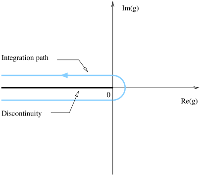
Figure 1: Contour integration in the complex coupling constant plane for the large orders asymptotics

For large positive $k$ this integral is dominated by the small $g$ behavior of the discontinuity, where semi-classical methods are expected to be applicable. Indeed, it turns out that for small real negative $g$, the discontinuity of $\mathfrak{Z}(g)$ is dominated by the contribution of a complex instanton (the real part of $\mathfrak{Z}(g)$ is still given by the contribution of the real classical solution). Therefore the small $g$ behavior of $\mathrm{Im}[\mathfrak{Z}(g)]$ is of the form

$$\mathrm{Im}[\mathfrak{Z}(-g+0_{+})]\ =\ C\,|g|^{\beta}\,\mathrm{e}^{-A|g|^{-\alpha}}\,\left[1+o(|g|^{*})\right]$$ (63)

with $A$ a number (corresponding to the instanton action $S_{\mathrm{inst}}$), $\alpha$ a (positive) constant given by power counting (in QM and standard local field theories $\alpha=1$), $C$ a number related to the determinant of the Hessian operator of fluctuations around the instanton, and $\beta$ a constant related to the number $m_{0}$ of zero-modes of the Hessian (in standard local field theories $\beta=1+m_{0}/2$). (See appendix C for details on the polymer case.)

Given (63), the integral (III.1.2) can be calculated: Changing variables from $g$ to $x:=g^{-\alpha}$, we obtain

$$\mathfrak{Z}_{k} = {(-1)^{k}}\frac{C}{\alpha\pi}\int_{0}^{\infty}\frac{\mathrm{d}x}{x}x^{(k-\beta)/\alpha}\mathrm{e}^{-Ax}$$ (64)

$$= (-1)^{k}\,{C\over\pi\alpha}\,A^{{\beta-k\over\alpha}}\,\Gamma\left({k-\beta\over\alpha}\right)$$

$\Gamma$ is Euler’s gamma function. Note that since (63) is valid for small $g$ only, this result is valid for large $k$. Using Stirling’s formula $\Gamma(n)\simeq n^{n}\mathrm{e}^{-n}\sqrt{{2\pi/n}}$, this amounts to

$$\mathfrak{Z}_{k}\ =\ (-1)^{k}\,\left[{k\over\alpha}\right]^{{k\over\alpha}}\,\left[A\mathrm{e}\right]^{\beta-k\over\alpha}\,\left[{k\over\alpha}\right]^{-{\beta\over\alpha}}\,{C\over\pi\alpha}\,\sqrt{{2\pi\alpha\over k}}\,\left[1+o(1/k^{*})\right]$$ (65)

and for $\alpha=1$

$$\mathfrak{Z}_{k}\ =\ (-1)^{k}\,{k}^{{k}}\,\left[{A\mathrm{e}}\right]^{\beta-k}\,{k}^{-{\beta}}\,{C\over\pi}\,\sqrt{{2\pi\over k}}\,\left[1+o(1/k^{*})\right]\ .$$ (66)

It is an alternating asymptotic series with a Borel transform with non-zero radius of convergence.

III.2 Instanton for the SAM

We are thus interested in the analytic structure of the partition function and the correlators of the SAM model for small negative coupling constant $b$

$$b<0\quad,\qquad b\to 0\ .$$ (67)

In particular we are interested in the discontinuity along the negative real axis. As shown in DavidWiese1998 this can be done more easily by first rescaling the fields and the size of the manifold with $b$ in an adequate way.

III.2.1 Complex rotation and rescalings for coupling constant and fields

We consider a finite manifold $\mathcal{M}$ with internal size $L$ defined as

$$\mathrm{Vol}(\mathcal{M})\ =\ L^{D}\ .$$ (68)

We are interested in the model for small complex coupling constant $b$, and more precisely in the discontinuity of the observables along the negative real axis ($b<0$ real), where there is a cut.

We denote the argument of the coupling constant $b$ by $\theta$

$$\theta=\mathrm{Arg}\left({b}\right)\ .$$ (69)

To reach the cut at negative $b$ from above or below amounts to taking the limit

$$\theta\ \to\ \pm\pi\qquad,\qquad|b|\ \mathrm{fixed}\ .$$ (70)

We now rescale the internal coordinate of the membrane $\mathsf{x}$ and the field $\mathsf{r}$ with the size $L$ of the manifold and the modulus $|b|$ of the coupling constant

$$\mathsf{x}\,\to\,|b|^{{1\over D-\epsilon}}L^{{D\over D-\epsilon}}\mathsf{x}\qquad,\qquad\mathsf{r}\,\to\,|b|^{{2-D\over 2(D-\epsilon)}}L^{{(2-D)D\over 2(D-\epsilon)}}\mathsf{r}$$ (71)

so that we now deal with a rescaled manifold $\mathcal{M}_{s}$ with internal size and internal volume

$$\mathrm{size}(\mathcal{M}_{s})\,=\,|b|^{-{1\over D-\epsilon}}L^{-{\epsilon\over D-\epsilon}}\qquad,\qquad\mathrm{Vol}(\mathcal{M}_{s})\,=\,|b|^{-{D\over D-\epsilon}}L^{-{\epsilon D\over D-\epsilon}}\ .$$ (72)

Similarly we must rescale the auxiliary fields $\rho$ and $V$ as

$$\rho\ \to\ |b|^{-1}L^{-D}\rho\qquad,\qquad V\ \to\ |b|^{-{D\over D-\epsilon}}L^{-{D^{2}\over D-\epsilon}}V\ .$$ (73)

The purpose of these rescalings is that as the original coupling constant $b$ goes to $0$, the effective theory for the auxiliary field $V$ becomes simple. Indeed it appears that both terms in the effective action $S[V]$ now scale in the same way, as will be detailed now.

Coupling constant:

Let us denote by $g$ the inverse of the volume of the rescaled manifold

$$g\ =\ {1\over\mathrm{Vol}(\mathcal{M}_{s})}\ =\ |b|^{{D\over D-\epsilon}}\,L^{{D\epsilon\over D-\epsilon}}$$ (74)

$g$ is the (dimensionless) effective coupling constant of the theory, which is real and positive and goes to 0 with $|b|$ as long as $\epsilon<D$.

Partition function:

The original partition function (for the manifold $\mathcal{M}$) becomes for the rescaled theory involving the manifold $\mathcal{M}_{s}$

$$Z_{\mathcal{M}_{s}}(b) = \int\mathcal{D}[{\mathsf{r}}]\,\mathcal{D}[{V}]\,\exp\left(-\int_{\mathcal{M}_{s}}\left(\frac{1}{2}(\nabla_{\!\mathsf{x}}\mathsf{r})^{2}+V(\mathsf{r})\right)\,+\,\,{\mathrm{e}^{-\mathrm{i}\theta}\over 2g}\int_{\mathsf{r}}V(\mathsf{r})^{2}\right)$$ (75)

$$= \int\mathcal{D}[V]\,\exp\left(-\,F_{\mathcal{M}_{s}}[{V}]\,+\,\,{\mathrm{e}^{-\mathrm{i}\theta}\over 2g}\int_{{\mathsf{r}}}{V}({\mathsf{r}})^{2}\right)\ .$$

Due to (74) both terms in the exponential scale as $\mathrm{Vol}(\mathcal{M}_{s})=1/g$.

Functional measure:

The functional measure over the rescaled field ${V}$ is now normalized so that

$$\int\mathcal{D}[{V}]\,\exp\left({\mathrm{e}^{-\mathrm{i}\theta}\over 2g}\int_{{\mathsf{r}}}{V}({\mathsf{r}})^{2}\right)\ =\ 1\ .$$ (76)

Correlation functions:

The moments for the gyration radius of the manifold become in the rescaled effective theory

$$\mathsf{R_{gyr}^{(k)}} = b^{-2}\,L^{-2D}\,\left(L\,g^{{1\over D-\epsilon}}\right)^{{(2-D)(2d+k)\over 2}-2D}\,\int_{\mathsf{r}_{1}}\int_{\mathsf{r}_{2}}|\mathsf{r}_{1}-\mathsf{r}_{2}|^{k}\,V(\mathsf{r}_{1})\,V(\mathsf{r}_{2})$$

$$= \mathrm{e}^{-2\mathrm{i}\theta}\,\left(|b|L^{D}\right)^{{2-D\over 2(D-\epsilon)}\cdot k}\,\int_{\mathsf{r}_{1}}\int_{\mathsf{r}_{2}}|\mathsf{r}_{1}-\mathsf{r}_{2}|^{k}\,V(\mathsf{r}_{1})\,V(\mathsf{r}_{2})$$

Hence

$$\mathsf{R_{gyr}^{(k)}} = \mathrm{e}^{-2\mathrm{i}\theta}\,L^{{2-D\over 2}k}\ g^{\,{2-D\over 2D}k}\,\int_{\mathsf{r}_{1}}\int_{\mathsf{r}_{2}}|\mathsf{r}_{1}-\mathsf{r}_{2}|^{k}\,V(\mathsf{r}_{1})\,V(\mathsf{r}_{2})\ .$$ (77)

$L$ is the internal extension of the original manifold $\mathcal{M}$. This has the correct dimension $L^{\nu_{0}k}$ with $\nu_{0}=(2-D)/2$, since $[R^{(k)}]=[\mathsf{r}]^{k}$ and $[\mathsf{r}]=[x]^{{2-D}\over 2}$. Note that there is no additional phase for $\theta=\pm\pi$.

III.2.2 Semiclassical limit and the effective action $\mathcal{S}[V]$

Now come the crucial points:

1. As long as

   $$\epsilon<D$$

   taking the semiclassical limit $b\to 0$ amounts to taking both the small coupling limit $g\to 0$ in the rescaled theory and the thermodynamic limit (infinite volume) for the rescaled manifold

   $$b\to 0\qquad\Leftrightarrow\qquad g\to 0\ \ \mbox{and}\ \ \mathrm{Vol}\left({\mathcal{M}_{s}}\right)\to\infty$$

   for the rescaled manifold.

2. In this thermodynamic limit the free energy $F_{\mathcal{M}_{s}}[V]$ becomes proportional to the volume of the manifold

   $$F_{\mathcal{M}_{s}}[{V}]\ =\ \mathrm{Vol}\left({\mathcal{M}_{s}}\right)\,\mathcal{E}[{V}]\,+\,\cdots\ .$$ (78)

   The free energy density $\mathcal{E}[{V}]$ is defined as

   $$\mathcal{E}[{V}]\ :=\ \lim_{\mathrm{Vol}(\mathcal{M}_{s})\to\infty}{1\over{\mathrm{Vol}}(\mathcal{M}_{s})}\,F_{\mathcal{M}_{s}}[{V}]$$ (79)

   in the limit where the size of the manifold $\mathcal{M}_{s}$ is rescaled to $\infty$, and its shape kept fixed. In this limit, the manifold $\mathcal{M}_{s}$ becomes locally a flat $D$-dimensional Euclidean space $\mathbb{R}^{D}$:

   $${\mathcal{M}_{s}}\ \to\ \mathbb{R}^{D}\ .$$ (80)

   The free energy density $\mathcal{E}[V]$ is independent of the size and of the shape of the manifold and it is enough to compute it for the infinite flat manifold.

3. Moreover – and this is an important point – as long as we are interested in the contribution of potentials $V$ such that the manifold is “trapped” in $V$ (namely such that the free energy density $\mathcal{E}[V]<0$ is negative, i.e. such that there is a “bound state” in $V$) the neglected terms $+\cdots$ are expected to be exponentially small in $1/g$.

4. Finally, since

   $$\mathrm{Vol}(\mathcal{M}_{s})\ =\ {1\over g}$$ (81)

   in the limit $g\to 0$ the functional integral takes the standard form

   $$Z(b)\ \stackrel{{\scriptstyle g\to 0}}{{=}}\ \int\mathcal{D}[V]\,\exp\left[-\,{1\over g}\mathcal{S}[V]\right]\ ,$$ (82)

   where $g$ is given by (74), the measure is given by (76) and the effective action $\mathcal{S}[V]$ for the field $V$ is given by

   $$\mathcal{S}[V]\ =\ \mathcal{E}[V]-{\mathrm{e}^{-\mathrm{i}\theta}\over 2}\int V^{2}$$ (83)

   $\mathcal{E}[V]$ is the free energy density for an infinite flat manifold trapped in the potential $V$, and is given by (79).

III.2.3 The functional integral for negative $b$ and the instanton

We are interested in the imaginary part of the partition function $Z(b)$ for $b$ along the negative real axis, that is for

$$\theta\ \to\ \pm\,\pi\ .$$ (84)

In this limit the effective action $\mathcal{S}[V]$ for the rescaled theory is real

$$\mathcal{S}[V]\ =\ \mathcal{E}[V]\,+\,{1\over 2}\int V^{2}$$ (85)

and the measure over $V$ is also real, since it is normalized such that

$$\int\mathcal{D}[V]\,\exp\left[-\,{1\over 2g}\,\int V^{2}\right]\ =\ 1\ .$$ (86)

It is now the standard measure for a real white noise with variance $g$:

$$\langle V(\mathsf{r}_{1})V(\mathsf{r}_{2})\rangle\ =\ {g}\,\delta(\mathsf{r}_{1}-\mathsf{r}_{2})\ .$$ (87)

Thus we can chose for integration measure over $V$ the standard measure over real $V(\mathsf{r})$

$$\int\mathcal{D}[V]_{\theta=\pm\pi}\ =\ \int_{-\infty}^{\infty}\prod_{\mathsf{r}}\,{\mathrm{d}V(\mathsf{r})\over\sqrt{2\pi g\delta^{d}(0)}}\ .$$ (88)

The instanton $V^{\mathrm{inst}}$ is a non-trivial finite action extremum of the action $\mathcal{S}[V]$ and was found in DavidWiese1998 . The saddle-point equation is

$$0=\frac{\delta{\cal S}[V]}{\delta V(\mathsf{r})}=V(\mathsf{r})\,+\,\langle\rho(\mathsf{r})\rangle_{V}\ ,$$ (89)

where $\rho(\mathsf{r})$ is the manifold density at point $\mathsf{r}$

$$\rho(\mathsf{r})\ =\ {1\over\mathrm{Vol}(\mathcal{M})}\int\mathrm{d}^{D}\mathsf{x}\,\delta(\mathsf{r}-\mathsf{r}(\mathsf{x}))$$ (90)

and from now on we drop the index at $\mathcal{M}_{s}$. $\langle\cdots\rangle_{V}$ refers to the expectation value for the phantom manifold trapped in the external potential $V(\mathsf{r})$, that is with the action

$$\int_{\mathcal{M}}\mathrm{d}^{D}\mathsf{x}\,\left({1\over 2}\left(\nabla_{\mathsf{x}}\mathsf{r}\right)^{2}+V(\mathsf{r})\right)\ .$$ (91)

The “classical vacuum” is $V=0$ (free manifold). The instanton $V^{\mathrm{inst}}$ is a configuration of potential which is negative (potential well $V(\mathsf{r})<0$), spherically symmetric, with $V\to 0$ as $|\mathsf{r}|\to\infty$. The solution of the instanton equation and its properties have been studied in DavidWiese1998 .

III.3 Contribution of fluctuations around the instanton

III.3.1 Instanton zero modes

The Hessian matrix (second derivative of the action) is

$${{\mathcal{S}}^{\prime\prime}[V]}_{\mathsf{r}_{1}\mathsf{r}_{2}}\ =\ {\delta^{2}\mathcal{E}[V]\over\delta V(\mathsf{r}_{1})\delta V(\mathsf{r}_{2})}\ =\ \delta^{d}(\mathsf{r}_{1}-\mathsf{r}_{2})\,+\,\langle\rho(\mathsf{r}_{1})\rho(\mathsf{r}_{2})\rangle_{V}^{\mathrm{conn}}\ .$$ (92)

The instanton has $d$ translational zero modes, corresponding to the position of the center of gravity $\mathsf{r}_{0}$ of the instanton. Thus the Hessian has $d$ zero modes

$$V^{\mathrm{zero}}_{a}\ =\ \nabla_{a}V^{\mathrm{inst}}\qquad;\qquad{\mathcal{S}}^{\prime\prime}[V]\cdot V^{\mathrm{zero}}_{a}\ =\ 0\ .$$ (93)

According to the previous analysis, see Eq. (50), the metric on the instanton moduli space $\mathcal{M}=\mathbb{R}^{d}$, $\mathrm{d}s^{2}\ =\ h_{ab}\,\mathrm{d}\mathsf{r}_{0}^{a}\mathrm{d}\mathsf{r}_{0}^{b}$, is

$$h_{ab}\ =\ {1\over 2\pi g}\int\mathrm{d}^{d}\mathsf{r}\,V^{\mathrm{zero}}_{a}V^{\mathrm{zero}}_{b}\ =\ \delta_{ab}\,{1\over 2\pi\,g\,d}\int\mathrm{d}^{d}\mathsf{r}\,\left(\overrightarrow{\nabla}V^{\mathrm{inst}}\right)^{2}$$ (94)

(using rotational invariance). Therefore the measure over the instanton position $\mathsf{r}_{0}$ is

$$\mathrm{d}^{d}\mathsf{r}_{0}\,\left[{1\over 2\pi\,g\,d}\int\mathrm{d}^{d}\mathsf{r}\,\left(\overrightarrow{\nabla}V^{\mathrm{inst}}\right)^{2}\right]^{d/2}\ .$$

Hence the contribution of the instanton to the partition function will be (depending on whether $\theta=\mathrm{Arg}(b)=\pm\pi$)

$$Z(b)\ \ \stackrel{{\scriptstyle\text{instanton}}}{{\leftarrow\!\!\!-\!\!\!-\!\!\!-\!\!\!-\!\!\!-\!\!\!-\!\!\!-\!\!\!-\!\!\!-\!\!\!\!}}\ \ \mathbf{C}_{\pm}\int\mathrm{d}^{d}\mathsf{r}_{0}\,\left[{1\over 2\pi d\,g}\int_{\mathsf{r}}(\vec{\nabla}V)^{2}\right]^{d/2}\,\mathrm{e}^{-\frac{1}{g}\mathcal{S}[V]}\,\left[{\det}^{\prime}\bigl{(}{\mathcal{S}}^{\prime\prime}[V]\bigr{)}\right]^{-\frac{1}{2}}$$ (95)

with $\mathbf{C}_{\pm}$ a simple factor (usually 1 or an integer for a real instanton) giving the weight of the instanton in the functional integral.

One might also expect zero-modes associated to the rotational invariance of the theory. Such modes would indeed appear for a non-rotationally invariant instanton solution. As it will turn out, the instanton is rotationally invariant, such no such zero-modes exist.

III.3.2 Unstable eigenmode

However, as expected for a theory with the wrong sign of the coupling and as shown in DavidWiese1998 , the instanton has one unstable eigenmode $V^{-}(\mathsf{r})$. Thus the Hessian has one negative eigenvalue $\lambda^{-}$ and its determinant is real but negative: ${\det}^{\prime}(S^{\prime\prime})<0$. Therefore we expect that the factor $\mathbf{C}_{\pm}$ will be complex.

In fact, as this is the case for the instanton in the local $\phi^{4}$ field theory, the real part of $\mathbf{C}_{\pm}$ is not unambiguously defined, but depends on the resummation procedure used to define the contribution of the classical saddle-point $V=0$ in the functional integral (this is known as the Stokes phenomenon). However, the instanton gives the dominant contribution to the imaginary part of the functional integral, and one can show that

$$\mathrm{Im}\bigl{[}Z(b)\bigr{]}\ \ \stackrel{{\scriptstyle\text{instanton}}}{{\leftarrow\!\!\!-\!\!\!-\!\!\!-\!\!\!-\!\!\!-\!\!\!-\!\!\!-\!\!\!-\!\!\!-\!\!\!\!}}\ \ \mathbf{D}_{\pm}\int\mathrm{d}^{d}\mathsf{r}_{0}\,\left[{1\over 2\pi d\,g}\int_{\mathsf{r}}(\vec{\nabla}V)^{2}\right]^{d/2}\,\mathrm{e}^{-\mathcal{V}\,\mathcal{S}[V]}\,\left|{\det}^{\prime}\bigl{(}{\mathcal{S}}^{\prime\prime}[V]\bigr{)}\right|^{-\frac{1}{2}}$$ (96)

with the weight factor $D_{\pm}$

$$\mathbf{D}_{\pm}\ =\ \mp\,{\mathrm{i}\over 2}\ .$$ (97)

This result can be obtained by a more precise analysis of the respective position of the integration path and of the instanton solution in the space of complex potentials $V(\mathsf{r})\in\mathbb{C}$ as $\theta$ is rotated from $0$ to $\pm\pi$, using the steepest descent method. This is shown in Appendix B.

III.4 Final result for the instanton contribution

The final result for the imaginary part of the partition function at negative coupling is

$$\mathrm{Im}\,Z(b)\ =\ \mp\,\frac{1}{2}\int\mathrm{d}^{d}\mathsf{r}_{0}\,\left[{1\over 2\pi d\,g}\int_{\mathsf{r}}(\vec{\nabla}V)^{2}\right]^{d/2}\,\mathrm{e}^{-{1\over g}\,\mathcal{S}[V]}\,\bigl{|}{\det}^{\prime}\left({\mathcal{S}}^{\prime\prime}[V]\right)\bigr{|}^{-\frac{1}{2}}\ .$$ (98)

depending on whether $\mathrm{Arg}(b)=\pm\pi$. The infinite bulk volume factor $\int\mathrm{d}^{d}\mathsf{r}_{0}$ disappears (as it should) in the normalized partition function $\mathfrak{Z}=Z/Z_{0}$

$$\mathrm{Im}\,\mathfrak{Z}(b)\ =\ \mp\,\frac{1}{2}\,g^{-d/D}\,\left[{\mathrm{e}^{-\bar{\zeta}^{\prime}(0)}\over d}\int_{\mathsf{r}}(\vec{\nabla}V)^{2}\right]^{d/2}\,\mathrm{e}^{-{1\over g}\,\mathcal{S}[V]}\,\left|{\det}^{\prime}\left({\mathcal{S}}^{\prime\prime}[V]\right)\right|^{-\frac{1}{2}}\ ,$$ (99)

where $\tilde{\zeta}^{\prime}(0)$ was defined in (9). One must remember that

$$g\ =\ \big{(}|b|L^{-\epsilon}\big{)}^{{D\over D-\epsilon}}$$ (100)

and that $\mathsf{r}$ is in fact the dimensionless rescaled field $\widetilde{\mathsf{r}}=\mathsf{r}\left(|b|L^{D}\right)^{-{2-D\over 2(D-\epsilon)}}=\mathsf{r}\left(g\,L^{D}\right)^{-{2-D\over 2D}}$ defined in (71). We thus obtain for the discontinuity of the partition function $\mathcal{Z}(b)$ for a marked manifold with a fixed point (as defined by Eq.(13))

$$\mathrm{Im}\,\mathcal{Z}(b)\ =\ \mp\,\frac{1}{2}\,L^{-d{2-D\over 2}}\,g^{\ -{d\over D}}\,\left[{1\over 2\pi d}\int_{\mathsf{r}}(\vec{\nabla}V)^{2}\right]^{d/2}\,\mathrm{e}^{-{1\over g}\,\mathcal{S}[V]}\,\left|{\det}^{\prime}\left({\mathcal{S}}^{\prime\prime}[V]\right)\right|^{-\frac{1}{2}}\ .$$ (101)

For the $N$-point correlators ${\cal R}^{(N)}(\mathsf{r}_{1},\cdots,\mathsf{r}_{N};b)$ defined by (21) the result is more complicated since the $\mathsf{r}_{i}$’s are rescaled in the process $b\to g$. However he result takes a simple form for global quantities such as the moments of the radius of gyration of the manifold $\mathcal{R}_{\mathrm{gyr}}^{(k)}=\langle\mathsf{R_{gyr}^{(k)}}\rangle$ defined by (28)

$$\begin{split}\mathrm{Im}\,\mathcal{R}_{\mathrm{gyr}}^{(k)}\ =\ &\mp\,\frac{1}{2}\,L^{(k-d){2-D\over 2}}\,g^{-{d\over D}+k{2-D\over 2D}}\,\mathrm{e}^{-{1\over g}\,\mathcal{S}[V]}\times\\ \ &\ \times\,\left[{1\over 2\pi d}\int_{\mathsf{r}}(\vec{\nabla}V)^{2}\right]^{d/2}\,\big{|}{\det}^{\prime}\left({\mathcal{S}}^{\prime\prime}[V]\right)\big{|}^{-\frac{1}{2}}\,\left[\int_{\mathsf{r}_{1}}\int_{\mathsf{r}_{2}}|\mathsf{r}_{1}-\mathsf{r}_{2}|^{k}\,V(\mathsf{r}_{1})V(\mathsf{r}_{2})\right]\ .\end{split}$$ (102)

III.5 Large orders

In the rest of this article, we shall denote for simplicity

$$\mathfrak{S}=\mathcal{S}[V^{\mathrm{inst}}]\ ,\quad\mathfrak{D}\,=\,{\det}^{\prime}\left(\mathcal{S}[V^{\mathrm{inst}}]\right)\ ,\quad\mathfrak{L}\,=\,\log(\mathfrak{D})\ ,\quad\mathfrak{W}\,=\,\left[{1\over 2\pi d}\int_{\mathsf{r}}(\vec{\nabla}V^{\mathrm{inst}})^{2}\right]^{d/2}\ .$$ (103)

If no UV divergences were present at $\epsilon=0$, the final result at $\epsilon=0$ would be

$$\mathrm{Im}\,\mathcal{Z}(b)\ =\ \mp\,\frac{1}{2}\,L^{-2D}\,|b|^{{4\over 2-D}}\,\mathrm{e}^{-{1\over|b|}\mathfrak{S}}\,\mathfrak{W}\,|\mathfrak{D}|^{-{1\over 2}}\ .$$ (104)

Using the the arguments of Sect. III.1.2, in particular the dispersion relation (III.1.2) and (66), the large-order asymptotics for the perturbative expansion of $\mathcal{Z}(b)$

$$\mathcal{Z}(b)\ =\ \sum_{k=0}^{\infty}\mathcal{Z}_{k}\,b^{k}$$ (105)

would be ($\epsilon=0$)

$$\mathcal{Z}_{k}\ \simeq\ (-1)^{k}\,\Gamma\left(k-{4\over 2-D}\right)\,{1\over 2\pi}\,L^{-2D}\,\mathfrak{W}\,|\mathfrak{D}|^{-{1\over 2}}\,\mathfrak{S}^{{4\over 2-D}-k}$$ (106)

or equivalently ($\epsilon=0$)

$$\mathcal{Z}_{k}\ \simeq\ (-1)^{k}\,\Gamma\left(k-2-{d\over 2}\right)\,{1\over 2\pi}\,L^{-{4d\over 4+d}}\,\mathfrak{W}\,|\mathfrak{D}|^{-{1\over 2}}\,\mathfrak{S}^{2+{d\over 2}-k}\ ,$$ (107)

indicating that the Borel transform of $\mathcal{Z}(b)$ has a finite radius of convergence $\mathfrak{S}$. Of course the instanton normalization $\mathfrak{W}\,|\mathfrak{D}|^{-{1\over 2}}$ depends also on $d$.

IV UV Divergences and renormalization

We now discuss the UV divergences in the determinant factor for the instanton, and how they are renormalized. We remind the reader that at one loop in perturbation theory, for $0<\epsilon\leq D$ there is a divergence associated to the operator $\mathbb{I}$ (super-renormalizable case); for $\epsilon=0$ two divergences associated to the operators $(\nabla\mathsf{r})^{2}$ and $\delta^{d}\bigl{(}\mathsf{r}(\mathsf{x})-\mathsf{r}(\mathsf{y})\bigr{)}$ (renormalizable case). For $\epsilon<0$ the theory is not renormalizable. The model is always considered for $D<2$ and $\epsilon$ is given by

$$\epsilon=2D-{d\over 2}(2-D)\ .$$ (108)

IV.1 Series representation of the determinant for the fluctuations

The Hessian matrix $\mathcal{S}^{\prime\prime}$ is given by (92). We rewrite it as

$$\mathcal{S}^{\prime\prime}_{\mathsf{r}_{1}\mathsf{r}_{2}}\ =\ {1\mathrm{l}}_{\mathsf{r}_{1}\mathsf{r}_{2}}\,-\,\mathbb{O}_{\mathsf{r}_{1}\mathsf{r}_{2}}\quad,\quad{1\mathrm{l}}_{\mathsf{r}_{1}\mathsf{r}_{2}}\ =\ \delta^{d}(\mathsf{r}_{1}-\mathsf{r}_{2})$$ (109)

$$\mathbb{O}_{\mathsf{r}_{1}\mathsf{r}_{2}}\ =\ \lim_{\mathcal{M}\to\mathbb{R}^{D}}{1\over\text{Vol}(\mathcal{M})}\int_{\mathsf{x}_{1}}\int_{\mathsf{x}_{2}}{\bigl{\langle}\delta^{d}\bigl{(}\mathsf{r}_{1}-\mathsf{r}(\mathsf{x}_{1})\bigr{)}\delta^{d}\bigl{(}\mathsf{r}_{2}-\mathsf{r}(\mathsf{x}_{2})\bigr{)}\bigr{\rangle}}_{V}^{\text{conn}}\ ,$$ (110)

where $V$ is the instanton potential $V^{\text{inst}}$. $\mathbb{O}$ can be rewritten, using translational invariance $\mathsf{x}\to\mathsf{x}+\mathsf{x}_{0}$ when $\mathcal{M}\to\mathbb{R}^{D}$, and the saddle point equation for the instanton potential $V$

$$\mathbb{O}_{\mathsf{r}_{1}\mathsf{r}_{2}} = \int_{\mathbb{R}^{D}}\!\mathrm{d}^{D}\mathsf{x}\,{\bigl{\langle}\delta^{d}\bigl{(}\mathsf{r}_{1}-\mathsf{r}(0)\bigr{)}\delta^{d}\bigl{(}\mathsf{r}_{2}-\mathsf{r}(\mathsf{x})\bigr{)}\bigr{\rangle}}_{V}^{\text{conn}}$$ (111)

$$= \int_{\mathbb{R}^{D}}\!\mathrm{d}^{D}\mathsf{x}\,\left[{\bigl{\langle}\delta^{d}\bigl{(}\mathsf{r}_{1}-\mathsf{r}(0)\bigr{)}\delta^{d}\bigl{(}\mathsf{r}_{2}-\mathsf{r}(\mathsf{x})\bigr{)}\bigr{\rangle}}_{V}\,-\,{\bigl{\langle}\delta^{d}\bigl{(}\mathsf{r}_{1}-\mathsf{r}(0)\bigr{)}\big{\rangle}}_{V}{\big{\langle}\delta^{d}\bigl{(}\mathsf{r}_{2}-\mathsf{r}(\mathsf{x})\bigr{)}\bigr{\rangle}}_{V}\right]$$

$$= \int_{\mathbb{R}^{D}}\!\mathrm{d}^{D}\mathsf{x}\,\left[{\bigl{\langle}\delta^{d}\bigl{(}\mathsf{r}_{1}-\mathsf{r}(0)\bigr{)}\delta^{d}\bigl{(}\mathsf{r}_{2}-\mathsf{r}(\mathsf{x})\bigr{)}\bigr{\rangle}}_{V}\,-V(\mathsf{r}_{1})V(\mathsf{r}_{2})\right]\ .$$

Let us already note that such an integral is IR finite, since from clustering we expect that at large distances

$${\bigl{\langle}\delta^{d}\bigl{(}\mathsf{r}_{1}-\mathsf{r}(\mathsf{x})\bigr{)}\delta^{d}\bigl{(}\mathsf{r}_{2}-\mathsf{r}(\mathsf{y})\bigr{)}\bigr{\rangle}}_{V}^{\text{conn}}\ =\ \mathcal{O}\bigl{(}\exp(-|\mathsf{x}-\mathsf{y}|m)\bigr{)}\quad\text{when}\quad|\mathsf{x}-\mathsf{y}|\,\to\,\infty\ ,$$ (112)

where $m$ is the “mass gap” of the excitations for the manifold trapped in the instanton potential $V$.

We have seen that the operator $\mathcal{S}^{\prime\prime}$ has $d$ zero modes $V_{a}^{\text{zero}}\propto\nabla_{a}V^{\text{inst}}$, which, as discussed in section (III.1), are eigenvectors of $\mathbb{O}$ with eigenvalue $\lambda_{0}=1$, and one unstable eigenmode $V^{-}$, which is an eigenvector of $\mathbb{O}$ with eigenvalue $\lambda_{-}$ larger than $1$. For convenience, we normalize its $\mathrm{L}_{2}$ norm to 1. Let us denote $\mathbb{P}^{0}$ the projector on the zero-modes, and $\mathbb{P}^{-}$ the projector on the unstable mode

$${\mathbb{P}^{0}}_{\,\mathsf{r}_{1}\mathsf{r}_{2}}\ =\ {\sum_{a}V_{a}^{\text{zero}}(\mathsf{r}_{1})V_{a}^{\text{zero}}(\mathsf{r}_{2})}\ =\ {\overrightarrow{\nabla}V\otimes\overrightarrow{\nabla}V\over\int_{\mathsf{r}}\left(\overrightarrow{\nabla}V\right)^{2}}\quad,\quad{\mathbb{P}^{-}}_{\,\mathsf{r}_{1}\mathsf{r}_{2}}\ =\ {V_{-}(\mathsf{r}_{1})V_{-}(\mathsf{r}_{2})}$$ (113)

and $\mathbb{P}$ the sum

$$\mathbb{P}\ =\ \mathbb{P}^{0}\,+\,\mathbb{P}^{-}\ .$$ (114)

Apart from these eigenvalues, is is easy to see that all other eigenvalues of $\mathbb{O}$ are smaller than $1$, but positive. Indeed, from Eq.(110), $\mathbb{O}$ is a positive operator, since for any $f(\mathsf{r})$

$$f\cdot\mathbb{O}\cdot f\ =\ {1\over\text{Vol}(\mathcal{M})}\,\left<\left[\int_{\mathsf{x}}f\bigl{(}\mathsf{r}(\mathsf{x})\bigr{)}\right]^{2}\right>_{V}^{\text{conn}}\ >\ 0\ .$$ (115)

To compute the determinant of the fluctuations we treat separately the negative and zero modes from the rest. We write the logarithm of ${\det}^{\prime}[\mathcal{S}^{\prime\prime}]$

$$\mathfrak{L}\ =\ \log\big{(}{{\det}^{\prime}\left[\mathcal{S}^{\prime\prime}\right]}\big{)}\ =\ \log(1-\lambda_{-})\,+\,\mbox{tr}\left[(\mathbb{I}-\mathbb{P})\log(\mathbb{I}-\mathbb{O})\right]\ .$$ (116)

The first term is the contribution of the unstable mode (it has an imaginary part), the second term is the contribution of all other modes with $0<\lambda<1$. In this last term we can expand the $\log$ and obtain a convergent series

$$\mathfrak{L}\ =\ \log(1-\lambda_{-})\,-\,\sum_{k=1}^{\infty}{1\over k}\,L_{k}\quad,\quad L_{k}\ =\ \mbox{tr}\bigl{[}(\mathbb{I}-\mathbb{P})\mathbb{O}^{k}\bigr{]}\ =\ \mbox{tr}\left[\mathbb{O}^{k}\right]-d-\lambda_{-}^{k}\ ,$$ (117)

provided that each term is UV finite (that is the trace is well defined).

We now show that only the first two terms $k=1$ and $k=2$ are UV divergent, and require renormalization.

IV.2 UV divergences

IV.2.1 UV divergences in $\mathsf{r}$ and in $\mathsf{x}$ space

UV divergences in the determinant are expected to come from the high momentum eigenmodes of $\mathcal{S}^{\prime\prime}$. If we consider a potential $V=V^{\text{inst}}+V_{>}$, with $V_{>}$ a high momentum fluctuation, we expect that a phantom manifold trapped in $V$ will feel only weakly the small wavelength variations of $V$, so its free energy $\mathcal{E}[V]$ will depend only weakly on $V_{>}$. The other term $\int\mathrm{d}^{d}\mathsf{r}\,V^{2}(\mathsf{r})$ will be dominant in the variation of the effective action $\mathcal{S}[V]$. As a consequence, high momentum eigenmodes of $\mathcal{S}^{\prime\prime}$ will have eigenvalues close to $1$, that is will be eigenmodes of $\mathbb{O}$ with very small eigenvalues $\lambda\to 0$.

Therefore UV divergences will come from the contribution of the numerous eigenvalues of $\mathbb{O}$ close to $0$, that is from the divergence of the spectral density $\rho_{\mathbb{O}}(\lambda)$ of the operator $\mathbb{O}$ at $\lambda=0$. We shall show that $\rho_{\mathbb{O}}(\lambda)$ diverges as $\lambda^{\epsilon/D-3}$, and that

$$\mbox{tr}[\mathbb{O}]\quad\text{is UV divergent if}\ \epsilon\leq D\quad,\quad\mbox{tr}[\mathbb{O}^{2}]\quad\text{UV divergent if}\ \epsilon=0$$ (118)

and that higher powers $\mbox{tr}[\mathbb{O}^{k}]$ ($k\geq 3)$ are UV convergent.

The $\mbox{tr}[\cdot]$ amounts in our representation to an integral over $\mathsf{r}$ in bulk space $\mathbb{R}^{d}$. UV divergences will occur as short-distance singularities in $\mathsf{r}$ space. We shall also see that to analyze the UV divergences it is more convenient to come back to the equivalent representation of $\mathbb{O}$ in $\mathsf{x}$ space (internal manifold).

IV.2.2 $\mbox{tr}[\mathbb{O}]$:

This term is given by

$$\mbox{tr}[\mathbb{O}]\ =\ \int\mathrm{d}^{d}\mathsf{r}\ \mathbb{O}_{\mathsf{r}\mathsf{r}}$$ (119)

and is UV divergent for $\epsilon\leq D$ because we expect that

$$\mathbb{O}_{\mathsf{r}\mathsf{r}^{\prime}}\ \simeq\ {|\mathsf{r}-\mathsf{r}^{\prime}|}^{-d+{2(\epsilon-D)\over 2-D}}\quad\text{as}\quad\mathsf{r}-\mathsf{r}^{\prime}\,\to\,0\ .$$ (120)

The crucial point (to be proven later) is that the short-distance behavior of $\mathbb{O}_{\mathsf{r}\mathsf{r}^{\prime}}$ for a manifold in the background potential $V(\mathsf{r})$ does not depend on the details of the potential $V$, and is given (at leading order) by that of a free manifold in a constant potential ($V(\mathsf{r})=V_{0}$). We can compute explicitly $\mathbb{O}_{\mathsf{r}\mathsf{r}^{\prime}}$ in that case and find Eq. (120).

Using (111) we can rewrite $\mbox{tr}[\mathbb{O}]$ as an $\mathsf{x}$-integral over the manifold $\mathcal{M}$, and integrate explicitly over $\mathsf{r}$, with the result

$$\begin{split}\mbox{tr}[\mathbb{O}]\ &=\ \int\mathrm{d}^{d}\mathsf{r}\ \int_{\mathcal{M}}\!\!\!\!\mathrm{d}^{D}\mathsf{x}\,\Bigl{[}{\bigl{\langle}\delta^{d}\bigl{(}\mathsf{r}-\mathsf{r}(\mathsf{x}_{0})\bigr{)}\delta^{d}\bigl{(}\mathsf{r}-\mathsf{r}(\mathsf{x})\bigr{)}\bigr{\rangle}_{V}-V(\mathsf{r})^{2}}\Bigr{]}\\ &=\ \int_{\mathcal{M}}\!\!\!\!\mathrm{d}^{D}\mathsf{x}\,\Bigl{[}{\bigl{\langle}\delta^{d}\bigl{(}\mathsf{r}(\mathsf{x})-\mathsf{r}(\mathsf{x}_{0})\bigr{)}\bigr{\rangle}_{V}\,-\,\int_{\mathsf{r}}V(\mathsf{r})^{2}}\Bigr{]}\ .\end{split}$$ (121)

It contains the integral of the correlation function

$$\langle{\delta^{d}\bigl{(}\mathsf{r}(\mathsf{x})-\mathsf{r}(\mathsf{x}_{0})\bigr{)}\rangle}_{V}$$ (122)

for a phantom manifold (i.e. without self-interaction) trapped in the instanton potential $V(\mathsf{r})$. The choice of the “origin” $\mathsf{x}_{0}$ is arbitrary, since (122) depends only on $\mathsf{x}-\mathsf{x}_{0}$ (translational invariance in $\mathcal{M}=\mathbb{R}^{D}$).

This integral is IR convergent, as can be seen from Eq. (112). UV divergences occur if the $\mathsf{x}$-integral is divergent at short distances on the manifold, i.e. for $|\mathsf{x}-\mathsf{x}_{0}|\to 0$. The correlation function (122) is very similar to the 2-point correlation function which appears at first order in the perturbative expansion of the self-avoiding manifold model, and more precisely for the normalized partition function $\mathfrak{Z}(b)$

$$\mathfrak{Z}(b)=1-{b\over 2}\,\int_{\mathsf{x},\mathsf{y}}\!{\bigl{\langle}\delta^{d}\bigl{(}\mathsf{r}(\mathsf{x})-\mathsf{r}(\mathsf{y})\bigr{)}\bigr{\rangle}}_{0}+{b^{2}\over 8}\,\int_{\mathsf{x},\mathsf{y},\mathsf{x}^{\prime},\mathsf{y}^{\prime}}\!{\bigl{\langle}\delta^{d}\bigl{(}\mathsf{r}(\mathsf{x})-\mathsf{r}(\mathsf{y})\bigr{)}\,\delta^{d}\bigl{(}\mathsf{r}(\mathsf{x}^{\prime})-\mathsf{r}(\mathsf{y}^{\prime})\bigr{)}\bigr{\rangle}}_{0}+\mathcal{O}(b^{3})\ .$$ (123)

One therefore expects that the renormalization group counter-terms at leading order, which subtract the leading order UV-divergences in (123) are also sufficient to render (121) finite. That this is indeed the case will be shown below.

IV.2.3 $\mbox{tr}[\mathbb{O}^{2}]$:

Similarly, starting from (111), we can rewrite $\mbox{tr}[\mathbb{O}^{2}]$ in term of two “replicas” of the manifold, labeled $\mathcal{M}_{1}$ and $\mathcal{M}_{2}$, fluctuating independently in the same instanton potential $V$ (without interactions). If we denote $\mathsf{r}_{1}(\mathsf{x})$ and $\mathsf{r}_{2}(\mathsf{x})$ the $\mathsf{r}$-fields for the two replicas, we have

$$\begin{split}\mbox{tr}[\mathbb{O}^{2}]\ =\ &\int\!\mathrm{d}^{d}\mathsf{r}\int\!\mathrm{d}^{d}{\mathsf{r}^{\prime}}\ \mathbb{O}_{\mathsf{r}\mathsf{r}^{\prime}}\mathbb{O}_{\mathsf{r}^{\prime}\mathsf{r}}\ \\ =\ &\int\!\mathrm{d}^{d}\mathsf{r}\int\!\mathrm{d}^{d}{\mathsf{r}^{\prime}}\,\int_{\mathcal{M}_{1}}\!\!\!\mathrm{d}^{D}\mathsf{x}\int_{\mathcal{M}_{2}}\!\!\!\mathrm{d}^{D}\mathsf{y}\,\Bigl{[}{\bigl{\langle}\delta^{d}(\mathsf{r}-\mathsf{r}_{1}(\mathsf{x}_{0}))\delta^{d}(\mathsf{r}^{\prime}-\mathsf{r}_{1}(\mathsf{x}))\bigr{\rangle}_{V}-V(\mathsf{r})V(\mathsf{r}^{\prime})}\Bigr{]}\times\\ &\hskip 133.72786pt\times\bigl{[}{\bigl{\langle}\delta^{d}(\mathsf{r}^{\prime}-\mathsf{r}_{2}(\mathsf{y}_{0}))\delta^{d}(\mathsf{r}-\mathsf{r}_{2}(\mathsf{y}))\bigr{\rangle}_{V}-V(\mathsf{r}^{\prime})V(\mathsf{r})}\bigr{]}\\ =\ &\int_{\mathcal{M}_{1}}\!\!\mathrm{d}^{D}\mathsf{x}\int_{\mathcal{M}_{2}}\!\!\mathrm{d}^{D}\mathsf{y}\,\left\{{\Bigl{\langle}\delta^{d}\bigl{(}\mathsf{r}_{1}(\mathsf{x}_{0})-\mathsf{r}_{2}(\mathsf{y})\bigr{)}\,\delta^{d}\bigl{(}\mathsf{r}_{1}(\mathsf{x})-\mathsf{r}_{2}(\mathsf{y}_{0})\bigr{)}\Bigr{\rangle}_{V}\vphantom{\left[\int_{\mathsf{r}_{1}}V(\mathsf{r})^{2}\right]^{2}}}\right.\\ &\hskip 28.45274pt\left.\,-\,\bigl{\langle}V(\mathsf{r}_{1}(\mathsf{x}_{0}))V(\mathsf{r}_{1}(\mathsf{x}))\bigr{\rangle}_{V}\,-\,\bigl{\langle}V(\mathsf{r}_{2}(\mathsf{y}_{0}))V(\mathsf{r}_{2}(\mathsf{y}))\bigr{\rangle}_{V}\,+\,\left[\int_{\mathsf{r}}V(\mathsf{r})^{2}\right]^{2}\right\}\ .\end{split}$$ (124)

The choice of the origins $\mathsf{x}_{0}$ and $\mathsf{y}_{0}$ on the two manifolds $\mathcal{M}_{1}$ and $\mathcal{M}_{2}$ is arbitrary.

This integral is IR finite by the same arguments as those for $\mbox{tr}[\mathbb{O}]$. UV divergences are only present in the first correlation function

$$\Bigl{\langle}\delta^{d}\bigl{(}\mathsf{r}_{1}(\mathsf{x}_{0})-\mathsf{r}_{2}(\mathsf{y})\bigr{)}\,\delta^{d}\bigl{(}\mathsf{r}_{1}(\mathsf{x})-\mathsf{r}_{2}(\mathsf{y}_{0})\bigr{)}\Bigr{\rangle}_{V}$$ (125)

very similar to the correlation function which appears at second order in $\mathfrak{Z}(b)$, see Eq. (123). We shall see that UV divergences occur when

$$\mathsf{x}\to\mathsf{x}_{0}\quad,\quad\mathsf{y}\to\mathsf{y}_{0}\qquad\text{simultaneously}$$ (126)

while the other terms $\bigl{\langle}V\bigl{(}\mathsf{r}(\mathsf{x})\bigr{)}V\bigl{(}\mathsf{r}(\mathsf{x}_{0})\bigr{)}\bigr{\rangle}_{V}$ are not singular.

IV.2.4 $\mbox{tr}[\mathbb{O}^{k}]$, $k\geq 3$:

We can similarly write the higher order terms. At order $k$ we need $k$ copies $\mathcal{M}_{\alpha}$ of the manifold $\mathcal{M}$, fluctuating in the same instanton potential $V(\mathsf{r})$. The most UV singular term in the $\mathsf{x}$-representation of $\mbox{tr}[\mathbb{O}^{k}]$ is

$$\int_{\otimes\mathcal{M}_{\alpha}}\hskip-4.30554pt\mathrm{d}^{D}\mathsf{x}\Bigl{<}\prod_{\alpha=1}^{k}\delta^{d}\bigl{(}\mathsf{r}_{\alpha-1}(\mathbf{o}_{\alpha-1})-\mathsf{r}_{\alpha}(\mathsf{x}_{\alpha}\bigr{)}\Bigr{>}_{V}$$ (127)

(where we identify $\alpha=0$ with $\alpha=k$), that we can represent graphically as a “necklace of $k$ manifolds”. The reference points $\mathbf{o}_{\alpha}$ on each $\mathcal{M}_{\alpha}$ can be chosen arbitrarily, for instance fixed to the origin. UV divergences occur when all pairs of points $(\mathbf{o}_{\alpha},\mathsf{x}_{\alpha})$ collapse simultaneously on each $\mathcal{M}_{\alpha}$. These terms are in fact UV finite for $\epsilon=0$.

Figure 2: Diagrammatic representation of the UV divergent correlation functions at order $k=1$ (one manifold), $k=2$ (2 manifolds), and $k=3$ (3 manifolds).

IV.3 MOPE for manifold(s) in a background potential

In DDG3 , GBU the UV divergences of the self-avoiding manifold model have been analyzed using a Multilocal Operator Product Expansion (MOPE). This formalism was developed to study the correlation function of multilocal operators of the form (19),

$$\bigl{<}\prod_{i}\delta^{d}\bigl{(}\mathsf{r}(\mathsf{x}_{i})-\mathsf{r}(\mathsf{y}_{i})\bigr{)}\bigr{>}_{0}\ ,$$ (128)

where the expectation values $\bigl{<}\cdots\bigr{>}_{0}$ are calculated for a free manifold model ($V=0$). We show here how this formalism can be adapted to deal with expectation values $\bigl{<}\cdots\bigr{>}_{V}$ for manifolds trapped in a non-zero background potential $V(\mathsf{r})$.

IV.3.1 Normal product decomposition of the potential $V$

In order to compute easily expectation values of operators in the background potential $V$, we shall use the normal product formalism already developed in DavidWiese1998 .

For simplicity we consider a potential $V(\mathsf{r})$ spherically symmetric (as the instanton potential) with its minimum at $\mathsf{r}=0$, of the form

$$V(\mathsf{r})\ =\ \sum_{n=0}^{\infty}{v_{n}\over{2}^{n}n!}\left(\mathsf{r}^{2}\right)^{n}\quad,\quad v_{1}\,=\,m_{0}^{2}\,>\,0\ \quad m_{0}\,=\,\text{``bare mass''}\ .$$ (129)

We may (at least formally), compute expectation values of operators $\bigl{<}\cdots\bigr{>}_{V}$ in perturbation theory, starting from the Gaussian potential $V(\mathsf{r})={m_{0}^{2}\over 2}\mathsf{r}^{2}$ and expanding in powers of the non-linear couplings $\{v_{k},\,k\geq 2\}$. This perturbation theory involves Feynman diagrams with massive propagators $1/(p^{2}+m_{0}^{2})$. It is more convenient to resum all tadpole diagrams and to deal with an expansion of the potential $V(\mathsf{r})$ in terms of normal products ${:\!\left(\mathsf{r}^{2}\right)^{n}\!:}_{m}$. The normal product ${:\![\ ]\!:}_{\mu}$ with the subtraction mass scale $\mu$ is defined by the global formula (expanded in $\mathsf{k}$, it generates all operators which are local powers of $\mathsf{r}$)

$${:\!\mathrm{e}^{\mathrm{i}\mathsf{k}\mathsf{r}}\!:}_{\mu}\ =\ \mathrm{e}^{\mathsf{k}^{2}G_{\mu}/2}\,\mathrm{e}^{\mathrm{i}\mathsf{k}\mathsf{r}}\ \ ,$$ (130)

where $G_{\mu}$ is the tadpole amplitude evaluated with the propagator of mass $\mu$,

$$G_{\mu}\ =\ \int{\mathrm{d}^{D}\mathsf{p}\over(2\pi)^{D}}\,{1\over\mathsf{p}^{2}+\mu^{2}}\ =\ {\Gamma\left({2-D\over 2}\right)\over(4\pi)^{D/2}}\,\mu^{D-2}\ .$$ (131)

Thus we rewrite the potential $V(\mathsf{r})$ given in (129) as

$$V(\mathsf{r})\ =\ \sum_{n=0}^{\infty}{g_{n}\over{2}^{n}n!}:\!{(\mathsf{r}^{2})}^{n}\!:_{m}\ .$$ (132)

The mass scale $m$ used to define the normal product ${:\!\cdots\!:}_{m}$ is defined self-consistently from $V$ so that it coincides with the “renormalized mass” in (132)

$$g_{1}\ =\ m^{2}\ .$$ (133)

This gives a self-consistent equation for $m$ in terms of $V(\mathsf{r})$ (or its Fourier transform $\hat{V}(\mathsf{k})$)

$$\begin{split}m^{2}\,&=\,-\,{1\over d}\int{\mathrm{d}^{d}\mathsf{k}\over(2\pi)^{d}}\,\mathsf{k}^{2}\,\widehat{V}(\mathsf{k})\,\mathrm{e}^{-{\mathsf{k}^{2}\over 2}G_{m}}\\ &=\ -\,{1\over G_{m}}\,(2\pi G_{m})^{-d/2}\ \int\mathrm{d}^{d}\mathsf{r}\,V(\mathsf{r})\left(1-{\mathsf{r}^{2}\over d\,G_{m}}\right)\,\mathrm{e}^{-{\mathsf{r}^{2}\over 2\,G_{m}}}\ .\end{split}$$ (134)

All other couplings $g_{0}$, $g_{2}$, $g_{3}$, etc. in (132) are then uniquely defined from the potential $V$. We rewrite $V$ as

$$V(\mathsf{r})=g_{0}+{m^{2}\over 2}:\!\mathsf{r}^{2}\!:+\,U(\mathsf{r})\quad;\quad U(\mathsf{r})\,=\,{g_{2}\over 2^{2}2!}:\!(\mathsf{r}^{2})^{2}\!:+{g_{3}\over 2^{3}3!}:\!(\mathsf{r}^{2})^{3}\!:+\dots$$ (135)

and we shall treat the non-linear terms $U(\mathsf{r})$ as perturbation. The expectation value of a (multilocal) operator $O(\mathsf{x}_{1},\dots,\mathsf{x}_{K})$ can be expanded as

$${\langle O(\mathsf{x}_{1},\dots,\mathsf{x}_{K})\rangle}_{V}=\sum_{N=0}^{\infty}{(-1)^{N}\over N!}\int\prod_{i=1}^{N}\mathrm{d}^{D}\mathsf{z}_{i}{\langle O(\mathsf{x}_{1},\dots,\mathsf{x}_{K})\,U(\mathsf{z}_{1})\cdots U(\mathsf{z}_{N})\rangle}_{m}^{\mathrm{connected}}\ ,$$ (136)

where $\langle\cdots\rangle$ is the expectation value in the massive free theory ($U=0$).

In this new perturbative expansion there are no tadpole diagrams. This makes the diagramatics much simpler. In addition many simplifications occur in the limit $d\to\infty$, as already noted in DavidWiese1998 .

IV.3.2 MOPE in a harmonic potential

First we consider the case of a potential quadratic in $\mathsf{r}$, which is especially simple. The potential reads

$$V(\mathsf{r})\ =\ v_{0}\,+\,{m_{0}^{2}\over 2}\mathsf{r}^{2}\ =\ g_{0}\,+\,{m^{2}\over 2}{:\!\mathsf{r}^{2}\!:}_{m}\quad,\quad m_{0}\,=\,m\quad;\quad v_{0}\ =\ g_{0}\,-\,d\,{m^{2}\over 2}\,G_{m}\ .$$ (137)

The field $\mathsf{r}$ is still free but massive with mass $m$ and the propagator is

$$G_{m}(\mathsf{x}-\mathsf{y})\ =\ \int{\mathrm{d}^{D}\mathsf{p}\over(2\pi)^{D}}\,{\mathrm{e}^{i\mathsf{p}(\mathsf{x}-\mathsf{y})}\over\mathsf{p}^{2}+m^{2}}\ =\ {1\over 2\pi}\,\left[{m\over 2\pi|\mathsf{x}-\mathsf{y}|}\right]^{{D-2\over 2}}\,K_{{D-2\over 2}}(m|\mathsf{x}-\mathsf{y}|)\ ,$$ (138)

where $K_{\nu}$ is the modified Bessel Function.

It is simple to study the short-distance limit of products of local and multilocal operators in this massive Gaussian theory, using exactly the same ideas and techniques as for the free massless case ($m=0$) developed in GBU .

OPE for the massive propagator $G_{m}$:

We express the short-distance expansion of multilocal operators in terms of the expansion for the massive propagator

$$G_{m}(\mathsf{x}-\mathsf{y})\ =\ c_{0}(D)\,m^{D-2}\,-\,d_{0}(D)\,|\mathsf{x}-\mathsf{y}|^{2-D}\,+\,c_{1}(D)\,m^{D}\,|\mathsf{x}-\mathsf{y}|^{2}\,-\,d_{1}(D)\,m^{2}\,|\mathsf{x}-\mathsf{y}|^{4-D}\,+\,\cdots\ .$$ (140)

The coefficients $c_{0}$, $c_{1}$, $d_{0}$, $d_{1}$, are finite as long as $D<2$ and are given by

$$c_{0}(D)={\Gamma\!\left({2-D\over 2}\right)\over(4\pi)^{D/2}}\ ,\quad c_{1}(D)={c_{0}(D)\over 2D}\ ,\quad d_{0}(D)=-{\Gamma\!\left({D-2\over 2}\right)\over 4\ \pi^{D/2}}\ ,\quad d_{1}(D)={d_{0}(D)\over 2(4-D)}\ .$$ (141)

Note that

$$d_{0}(D)={1\over(2-D)\mathcal{S}_{D}}\quad\text{with}\quad\mathcal{S}_{D}={2\,\pi^{{D\over 2}}\over\Gamma(D/2)}\ =\ \text{volume of the unit sphere in}\ \mathbb{R}^{D}\ .$$ (142)

This expansion follows itself from the OPE for the product of two $\mathsf{r}$ fields in the massive theory, which reads

$$\mathsf{r}^{a}(\mathsf{x})\mathsf{r}^{b}(\mathsf{y})\,=\,-|\mathsf{x}-\mathsf{y}|^{2-D}\,d(|\mathsf{x}-\mathsf{y}|^{2}m^{2})\,\delta^{ab}\,{1\mathrm{l}}+\sum_{p_{1},p_{1}}{\mathsf{x}^{p_{1}}\over p_{1}!}{\mathsf{y}^{p_{2}}\over p_{2}!}:\!\nabla^{p_{1}}\mathsf{r}^{a}\nabla^{p_{2}}\mathsf{r}^{b}\!:_{0}\ ,$$ (143)

where the coefficient $d(|\mathsf{x}-\mathsf{y}|^{2}m^{2})$ has an (asymptotic) series expansion in $|\mathsf{x}-\mathsf{y}|^{2}m^{2}$

$$d(|\mathsf{x}-\mathsf{y}|^{2}m^{2})=d_{0}+d_{1}|\mathsf{x}-\mathsf{y}|^{2}m^{2}+d_{2}|\mathsf{x}-\mathsf{y}|^{4}m^{4}+\cdots$$

and where the normal products $:\!\cdots\!:_{0}$ with respect to the zero mass means that the operators $\nabla^{\bullet}\mathsf{r}\nabla^{\bullet}\mathsf{r}$ are defined through dimensional regularization (see below).

MOPE for $\delta^{d}(\mathsf{r}_{1}-\mathsf{r}_{1}^{\prime})$ and $\mbox{${\mbox{tr}}$}[\mathbb{O}]$:

We first consider the short-distance expansion for the operator $\delta^{d}(\mathsf{r}(\mathsf{x})-\mathsf{r}(\mathsf{y}))$, which enters in $\mathrm{\mbox{tr}}[\mathbb{O}]$. Using the definition (130) for the normal product we can write it as

$$\begin{split}\delta^{d}(\mathsf{r}(\mathsf{x})-\mathsf{r}(\mathsf{y}))\ &=\ \int{\mathrm{d}^{d}\mathsf{k}\over(2\pi)^{d}}\,\mathrm{e}^{\mathrm{i}\mathsf{k}(\mathsf{r}(\mathsf{x})-\mathsf{r}(\mathsf{y}))}\\ &=\ \int{\mathrm{d}^{d}\mathsf{k}\over(2\pi)^{d}}\,\mathrm{e}^{-\mathsf{k}^{2}\bigl{(}G_{m}(0)-G_{m}(\mathsf{x}-\mathsf{y})\bigr{)}}\,:\!\mathrm{e}^{\mathrm{i}\mathsf{k}(\mathsf{r}(\mathsf{x})-\mathsf{r}(\mathsf{y}))}\!:_{m}\ .\end{split}$$ (144)

The last bilocal operator is regular at short distance (when $\mathsf{x}\to\mathsf{y}$) and can be expanded in $\mathsf{x}-\mathsf{y}$ as

$$:\!\mathrm{e}^{\mathrm{i}k(\mathsf{r}(x)-\mathsf{r}(\mathsf{y}))}\!:_{m}\ =\ {1\mathrm{l}}(\mathsf{z})\,-\,{1\over 2}\mathsf{k}_{a}\mathsf{k}_{b}\,(\mathsf{x}^{\mu}-\mathsf{y}^{\mu})(\mathsf{x}^{\nu}-\mathsf{y}^{\nu})\,:\nabla_{\mu}\mathsf{r}^{a}\nabla_{\nu}\mathsf{r}^{b}(\mathsf{z}):_{m}\,+\,\cdots\ ,$$ (145)

where $\mathsf{z}={\mathsf{x}+\mathsf{y}\over 2}$ and the subdominant terms are of order $\mathcal{O}(|\mathsf{x}-\mathsf{y}|^{4})$ with higher derivative operators. We insert (145) into (144) and integrate over $\mathsf{k}$ to obtain

$$\begin{split}\delta^{d}(\mathsf{r}(\mathsf{x})-\mathsf{r}(\mathsf{y}))\ =\ (4\pi)^{-{d\over 2}}&\left[G_{m}(0)-G_{m}(\mathsf{x}-\mathsf{y})\right]^{-{d\over 2}}\ \times\\ \times&\left[{1\mathrm{l}}(\mathsf{z})-{\delta_{ab}\over 4}{(\mathsf{x}^{\mu}-\mathsf{y}^{\mu})(\mathsf{x}^{\nu}-\mathsf{y}^{\nu})\over\left[G_{m}(0)-G_{m}(\mathsf{x}-\mathsf{y})\right]}:\!\nabla_{\mu}\mathsf{r}^{a}\nabla_{\nu}\mathsf{r}^{b}(\mathsf{z})\!:_{m}\,+\,\cdots\right]\ .\end{split}$$ (146)

We now use the short-distance expansion (140) of the massive propagator $G_{m}(\mathsf{x}-\mathsf{y})$ and insert it into (146) to obtain

$$\begin{split}\delta^{d}(\mathsf{r}(\mathsf{x}{-}\mathsf{r}(\mathsf{y}))=(4\pi\,d_{0})^{-{d\over 2}}|\mathsf{x}{-}\mathsf{y}|^{\epsilon-2D}\,\left[\!\left(1+{d\over 2}{c_{1}\over d_{0}}m^{D}|\mathsf{x}{-}\mathsf{y}|^{D}-{d\over 2}{d_{1}\over d_{0}}m^{2}|\mathsf{x}{-}\mathsf{y}|^{2}+\cdots\right){1\mathrm{l}}(\mathsf{z})\right.\\ -\left.{\delta_{ab}\over 4}{(\mathsf{x}^{\mu}-\mathsf{y}^{\mu})(\mathsf{x}^{\nu}-\mathsf{y}^{\nu})\over d_{0}\,|\mathsf{x}{-}\mathsf{y}|^{2-D}}{:\!\nabla_{\mu}\mathsf{r}^{a}\nabla_{\nu}\mathsf{r}^{b}(\mathsf{z})\!:}_{m}\,+\,\cdots\right]\ .\end{split}$$ (147)

In (147) we can regroup the two terms of order $|\mathsf{x}-\mathsf{y}|^{\epsilon-D}$ as

$$(4\pi\,d_{0})^{-d/2}\,|\mathsf{x}-\mathsf{y}|^{\epsilon-D}\,\left[{d\over 2}{c_{1}\over d_{0}}m^{D}\,{1\mathrm{l}}(\mathsf{z})\,-{1\over 4d_{0}}{(\mathsf{x}^{\mu}-\mathsf{y}^{\mu})(\mathsf{x}^{\nu}-\mathsf{y}^{\nu})\over|\mathsf{x}-\mathsf{y}|^{2}}\,{:\!\nabla_{\mu}\mathsf{r}\nabla_{\nu}\mathsf{r}(\mathsf{z})\!:}_{m}\right]\ .$$ (148)

Note that the OPE (147) is a relation between operators, and is valid for any choice of the mass $m$ used to define the normal product. Thus the term (148) can be rewritten as the normal ordered operator ${:\!\nabla\mathsf{r}\nabla\mathsf{r}\!}:_{0}$ with subtraction mass $\mu=0$

$$(4\pi\,d_{0})^{-d/2}\,|\mathsf{x}-\mathsf{y}|^{\epsilon-D}\,\left[-{1\over 4d_{0}}{(\mathsf{x}^{\mu}-\mathsf{y}^{\mu})(\mathsf{x}^{\nu}-\mathsf{y}^{\nu})\over|\mathsf{x}-\mathsf{y}|^{2}}\,{:\!\nabla_{\mu}\mathsf{r}\nabla_{\nu}\mathsf{r}(\mathsf{z})\!:}_{0}\right]\ .$$ (149)

Indeed we have the relation

$${:\!\nabla_{\mu}\mathsf{r}^{a}\nabla_{\nu}^{b}\mathsf{r}\!:}_{m}\ =\ {:\!\nabla_{\mu}\mathsf{r}^{a}\nabla_{\nu}^{b}\mathsf{r}\!:}_{0}\ -\ 2\,\delta^{ab}\,\delta_{\mu\nu}\,m^{D}\ c_{1}(D)\,{1\mathrm{l}}\ .$$ (150)

Since this relation will be crucial to prove renormalizability, let us show it explicitly. From the definition of the normal product we have

$${:\!\nabla_{\mu}\mathsf{r}^{a}\nabla_{\nu}^{b}\mathsf{r}\!:}_{m}\ =\ \nabla_{\mu}\mathsf{r}^{a}\nabla_{\nu}\mathsf{r}^{b}\ -\ {\langle\nabla_{\mu}\mathsf{r}^{a}\nabla_{\nu}\mathsf{r}^{b}\rangle}_{m}\,{1\mathrm{l}}$$ (151)

for any $m$, hence

$${:\!\nabla_{\mu}\mathsf{r}^{a}\nabla_{\nu}\mathsf{r}^{b}\!:}_{m}-:\!\nabla_{\mu}\mathsf{r}^{a}\nabla_{\nu}\mathsf{r}^{b}\!:_{0}\ =\ -\ \bigl{(}{\langle\nabla_{\mu}\mathsf{r}^{a}\nabla_{\nu}\mathsf{r}^{b}\rangle}_{m}-{\langle\nabla_{\mu}\mathsf{r}^{a}\nabla_{\nu}\mathsf{r}^{b}\rangle}_{0}\bigr{)}\,{1\mathrm{l}}\ .$$ (152)

The r.h.s. is easily calculated using the OPE (140) for the propagator $G_{m}$ itself, since

$$\langle\mathsf{r}^{a}(x)\mathsf{r}^{b}(y)\rangle_{m}\ =\ \delta^{ab}\,G_{m}(\mathsf{x}-\mathsf{y})\ .$$ (153)

This yields

$${\bigl{<}\nabla_{\mu}\mathsf{r}^{a}\nabla_{\nu}\mathsf{r}^{b}\bigr{>}}_{m}-{\bigl{<}\nabla_{\mu}\mathsf{r}^{a}\nabla_{\nu}\mathsf{r}^{b}\bigr{>}}_{0} = \delta^{ab}\,\left.{\partial\over\partial\mathsf{x}^{\mu}}{\partial\over\partial\mathsf{y}^{\nu}}\left[G_{m}(\mathsf{x}-\mathsf{y})-G_{0}(\mathsf{x}-\mathsf{y})\right]\right|_{\mathsf{x}=\mathsf{y}}$$ (154)

$$= -2\,\delta^{ab}\,\delta_{\mu\nu}\,m^{D}\ c_{1}(D)\ .$$

Note that the massless propagator $G_{0}(\mathsf{x}-\mathsf{y})$ is IR divergent but the IR divergent term is constant (independent of $\mathsf{x}-\mathsf{y}$) and disappears in (154) because of the $\mathsf{x}$ derivatives. Hence we obtain (150).

Thus we have obtained the first three terms of the MOPE for the $\delta$ operator in the $U=0$ background

$$\begin{split}\delta^{d}(\mathsf{r}(\mathsf{x})-\mathsf{r}(\mathsf{y}))\ =\ &(4\pi d_{0}(D))^{-{d\over 2}}|\mathsf{x}-\mathsf{y}|^{\epsilon-2D}\left[1-{d\over 4(4-D)}m^{2}|\mathsf{x}-\mathsf{y}|^{2}+\cdots\right]{1\mathrm{l}}(\mathsf{z})\\ -\,\pi\,(4\pi&d_{0}(D))^{-\left(1+{d\over 2}\right)}|\mathsf{x}-\mathsf{y}|^{\epsilon-D-2}(\mathsf{x}^{\mu}-\mathsf{y}^{\mu})(\mathsf{x}^{\nu}-\mathsf{y}^{\nu})\,{:\!\nabla_{\mu}\mathsf{r}\nabla_{\nu}\mathsf{r}\!:}_{0}\ +\ \cdots\ .\end{split}$$ (155)

The same argument can be used to construct the higher orders of the MOPE. They involve higher dimensional operators of the form $O_{p}={:\!\nabla^{p_{1}}\mathsf{r}\nabla^{p_{2}}\mathsf{r}\nabla^{p_{3}}\mathsf{r}\cdots\!:}_{0}$ (since the operator $\delta^{d}(\mathsf{r}(\mathsf{x})-\mathsf{r}(\mathsf{y}))$ is invariant by translation $\mathsf{r}\to\mathsf{r}+\mathsf{r}_{0}$ the $O_{p}$ must contain only derivatives $\nabla\mathsf{r}$, that is $p_{j}>0$, and by parity in $\mathsf{r}$ the $O_{p}$ must be even in $\mathsf{r}$). They give subdominant powers of $|\mathsf{x}-\mathsf{y}|$ of the form $m^{2k}|\mathsf{x}-\mathsf{y}|^{\epsilon-2D+2k+\sum_{j}{(p_{j}-1+D/2)}}$.

Finally let us stress that the two first terms of the MOPE (for $D<2$) are the terms of order $|\mathsf{x}-\mathsf{y}|^{\epsilon-2D}$ and $|\mathsf{x}-\mathsf{y}|^{\epsilon-D}$ and that they are the same as for the MOPE for the free membrane, that is for $m=0$. This will imply that the (one-loop) UV divergences (single poles at $\epsilon=D$ and $\epsilon=0$) due to this MOPE in the massive theory (self-avoiding manifold in a harmonic confining external potential) are canceled by the same counterterms as for the free theory (self-avoiding manifold with no confining potential). These counterterms are proportional to the operators ${1\mathrm{l}}$ and $(\nabla\mathsf{r})^{2}$.

MOPE for $\delta^{d}(\mathsf{r}_{1}-\mathsf{r}_{2})\delta^{d}(\mathsf{r}_{1}-\mathsf{r}_{2})$ and $\mbox{\rm\mbox{tr}}[\mathbb{O}^{2}]$:

The reader familiar with the techniques of GBU will see that the same arguments can be used to construct the MOPE for general products of local and multilocal operators in the $m\neq 0$, $U=0$ background.

Let us concentrate on the MOPE for two $\delta$ operators, which enters in $\mathrm{\mbox{tr}}[\mathbb{O}^{2}]$. We are interested in the short-distance expansion ($\mathsf{x}\to\mathsf{x}_{0}$, $\mathsf{y}\to\mathsf{y}_{0}$) for the product of two bilocal operators

$$\delta^{d}(\mathsf{r}_{1}(\mathsf{x}_{0})-\mathsf{r}_{2}(\mathsf{y}))\delta^{d}(\mathsf{r}_{1}(\mathsf{x})-\mathsf{r}_{2}(\mathsf{y}_{0}))\ ,$$ (156)

where $\mathsf{r}_{1}$ and $\mathsf{r}_{2}$ belong to two independent manifolds $\mathcal{M}_{1}$ and $\mathcal{M}_{2}$. As above, we write the $\delta$’s as a Fourier transform of an exponential and reexpress it in terms of normal products

$$\begin{split}&\delta^{d}(\mathsf{r}_{1}(\mathsf{x}_{0})-\mathsf{r}_{2}(\mathsf{y}))\delta^{d}(\mathsf{r}_{1}(\mathsf{x})-\mathsf{r}_{2}(\mathsf{y}_{0}))=\int\frac{\mathrm{d}^{d}\mathsf{k}_{1}\mathrm{d}^{d}\mathsf{k}_{2}}{(2\pi)^{2d}}\mathrm{e}^{\mathrm{i}\left(\mathsf{k}_{1}[\mathsf{r}_{1}(\mathsf{x}_{0})-\mathsf{r}_{2}(\mathsf{y})]+\mathsf{k}_{2}[\mathsf{r}_{1}(\mathsf{x})-\mathsf{r}_{2}(\mathsf{y}_{0})]\right)}\\ &=\int\frac{\mathrm{d}^{d}\mathsf{k}_{1}\mathrm{d}^{d}\mathsf{k}_{2}}{(2\pi)^{2d}}\,:\!\mathrm{e}^{\mathrm{i}\left({\mathsf{k}_{1}[\mathsf{r}_{1}(\mathsf{x}_{0})-\mathsf{r}_{2}(\mathsf{y})]+\mathsf{k}_{2}[\mathsf{r}_{1}(\mathsf{x})-\mathsf{r}_{2}(\mathsf{y}_{0})]}\right)}\!:\,\mathrm{e}^{-\mathsf{k}_{1}\mathsf{k}_{2}\left[G_{m}{(\mathsf{x}_{0}-\mathsf{x})}+G_{m}(\mathsf{y}-\mathsf{y}_{0})\right]-(\mathsf{k}_{1}^{2}+\mathsf{k}_{2}^{2})G_{m}(0)}\end{split}$$

Note that there are no cross-terms, as those proportional to $G(\mathsf{x}-\mathsf{y})$, since $\mathsf{x}$ and $\mathsf{y}$ belong to different manifolds, thus $\mathsf{r}_{1}(\mathsf{x})$ and $\mathsf{r}_{2}(\mathsf{y})$ are uncorrelated. We now keep the dominant term for the OPE when $\mathsf{x}\to\mathsf{x}_{0}$ and $\mathsf{y}\to\mathsf{y}_{0}$

$$:\!\mathrm{e}^{\mathrm{i}\left({\mathsf{k}_{1}[\mathsf{r}_{1}(\mathsf{x}_{0})-\mathsf{r}_{2}(\mathsf{y}_{0})]+\mathsf{k}_{2}[\mathsf{r}_{1}(\mathsf{x})-\mathsf{r}_{2}(\mathsf{y}_{0})]}\right)}\!:\ =\ :\!\mathrm{e}^{\mathrm{i}\left({(\mathsf{k}_{1}+\mathsf{k}_{2})[\mathsf{r}_{1}(\mathsf{x}_{0})-\mathsf{r}_{2}(\mathsf{y}_{0})]}\right)}\!:\,+\,\cdots$$

(the neglected terms contain subdominant $\nabla^{p}\mathsf{r}$’s), rewrite this term as

$$:\!\mathrm{e}^{\mathrm{i}\left({(\mathsf{k}_{1}+\mathsf{k}_{2})[\mathsf{r}_{1}(\mathsf{x}_{0})-\mathsf{r}_{2}(\mathsf{y}_{0})]}\right)}\!:\ =\ \mathrm{e}^{\mathrm{i}\left({(\mathsf{k}_{1}+\mathsf{k}_{2})[\mathsf{r}_{1}(\mathsf{x}_{0})-\mathsf{r}_{2}(\mathsf{y}_{0})]}\right)}\,\mathrm{e}^{(\mathsf{k}_{1}+\mathsf{k}_{2})^{2}G_{m}(0)}$$

and integrate over $\mathsf{k}_{1}$ and $\mathsf{k}_{2}$ to obtain

$$\begin{split}\int&\frac{\mathrm{d}^{d}\mathsf{k}_{1}\,\mathrm{d}^{d}\mathsf{k}_{2}}{(2\pi)^{2d}}\,:\!\mathrm{e}^{\mathrm{i}(\mathsf{k}_{1}+\mathsf{k}_{2})[\mathsf{r}_{1}(\mathsf{x}_{0})-\mathsf{r}_{2}(\mathsf{y}_{0})}\!:\,\mathrm{e}^{\mathsf{k}_{1}\mathsf{k}_{2}\left[2G_{m}(0)-G_{m}(\mathsf{x}_{0}-\mathsf{x})-G_{m}(\mathsf{y}-\mathsf{y}_{0})\right]}\\ &=\int\frac{\mathrm{d}^{d}\mathsf{k}\,\mathrm{d}^{d}\mathsf{k}^{\prime}}{(2\pi)^{2d}}\,\mathrm{e}^{i\mathsf{k}[\mathsf{r}_{1}(\mathsf{x}_{0})-\mathsf{r}_{2}(\mathsf{y}_{0})]}\mathrm{e}^{(k^{2}/4-{k^{\prime}}^{2})[2G_{m}(0)-G_{m}(\mathsf{x}_{0}-\mathsf{x})-G_{m}(\mathsf{y}-\mathsf{y}_{0})]}\end{split}$$ (157)

with $\mathsf{k}=\mathsf{k}_{1}+\mathsf{k}_{2}$ and $\mathsf{k}^{\prime}=(\mathsf{k}_{1}-\mathsf{k}_{2})/2$. The leading term is obtained by dropping the factor of $\mathsf{k}^{2}/4$ in the second exponential (the neglected terms give subdominant $\delta^{(n)}(\mathsf{r}_{1}-\mathsf{r}_{2})$ terms). This allows to do the integrations explicitly

$$\delta^{d}(\mathsf{r}_{1}(\mathsf{x}_{0})-\mathsf{r}_{2}(\mathsf{y}))\delta^{d}(\mathsf{r}_{1}(\mathsf{x})-\mathsf{r}_{2}(\mathsf{y}_{0})) \simeq \left(4\pi\right)^{-d/2}\left[2G_{m}(0)-G_{m}(\mathsf{x}-\mathsf{x}_{0})-G_{m}(\mathsf{y}-\mathsf{y}_{0})\right]^{-d/2}$$ (158)

$$\times\,\delta^{d}\left(\mathsf{r}_{1}(\mathsf{x}_{0})-\mathsf{r}_{2}(\mathsf{y}_{0})\right)\ .$$

From the short-distance expansion (140) for $G_{m}(0)-G_{m}(\mathsf{x})$ the most singular term when both $\mathsf{x}\to\mathsf{x}_{0}$ and $\mathsf{y}\to\mathsf{y}_{0}$ is

$$\delta^{d}(\mathsf{r}_{1}(\mathsf{x}_{0})-\mathsf{r}_{2}(\mathsf{y}))\delta^{d}(\mathsf{r}_{1}(\mathsf{x})-\mathsf{r}_{2}(\mathsf{y}_{0}))=\frac{\left[|\mathsf{x}-\mathsf{x}_{0}|^{2-D}+|\mathsf{y}-\mathsf{y}_{0}|^{2-D}\right]^{-d/2}}{(4\pi d_{0}(D))^{d/2}}\,\delta^{d}(\mathsf{r}_{1}(\mathsf{x}_{0})-\mathsf{r}_{2}(\mathsf{y}_{0}))\,+\,\cdots\ .$$ (159)

Thus we have obtained the leading term for the MOPE in the harmonic background $U=0$, $m\neq 0$.

This leading coefficient given by (159) is the same as for the free membrane ($V=0$). The same calculation can be done for the MOPE of two $\delta$’s on the same membrane, and we get (at leading order) a MOPE with the same coefficient

$$\delta^{d}(\mathsf{r}(\mathsf{x}_{0})-\mathsf{r}(\mathsf{y}))\delta^{d}(\mathsf{r}(\mathsf{x})-\mathsf{r}(\mathsf{y}_{0}))=\frac{\left[|\mathsf{x}-\mathsf{x}_{0}|^{2-D}+|\mathsf{y}-\mathsf{y}_{0}|^{2-D}\right]^{-d/2}}{(4\pi d_{0}(D))^{d/2}}\,\delta^{d}(\mathsf{r}(\mathsf{x}_{0})-\mathsf{r}(\mathsf{y}_{0}))\,+\,\cdots\ .$$ (160)

This implies in particular that the (one-loop) UV divergence (single pole at $\epsilon=0$) due to this MOPE in the massive theory (self-avoiding manifold in a harmonic confining external potential) is canceled by the same counterterm as for the free theory (self-avoiding manifold with no confining potential). This counterterm is proportional to the bilocal operator $\delta(\mathsf{r}-\mathsf{r}^{\prime})$.

MOPE for higher order terms and $\mathrm{\mbox{tr}}[\mathbb{O}^{k}]$:

The same analysis can be performed for the product of three $\delta$’s, in particular $\delta^{d}[\mathsf{r}_{1}(\mathsf{x}_{0})-\mathsf{r}_{2}(\mathsf{y})]\delta^{d}[\mathsf{r}_{2}(\mathsf{y}_{0})-\mathsf{r}_{3}(\mathsf{z})]\delta^{d}[\mathsf{r}_{3}(\mathsf{z}_{0})-\mathsf{r}_{1}(\mathsf{x})]$, which has to be considered for the quantity $\mathrm{\mbox{tr}}[\mathbb{O}^{3}]$. It shows that the leading singularity when $\mathsf{x}\to\mathsf{x}_{0}$, $\mathsf{y}\to\mathsf{y}_{0}$, $\mathsf{z}\to\mathsf{z}_{0}$ is given by the same MOPE as in the free theory, with the same leading coefficient. No additional UV divergences arise. The same result holds for higher order products of $\delta$’s.

IV.3.3 MOPE in the anharmonic potential

We now generalize this analysis to the SAM model in an anharmonic confining potential.

General discussion:

The perturbative expansion involves now interaction vertices given by the expansion of the local potential $U(\mathsf{r})$. For $D<2$ and as long as no bilocal $\delta(\mathsf{r}-\mathsf{r}^{\prime})$ operators are inserted this perturbation theory is UV finite. The only UV divergences that occur when $D\to 2$ are given by the tadpole amplitudes $G_{m}$, but they are subtracted by the normal product prescription $:\!\cdots\!:_{m}$. Thus as long as the normal ordered potential $V$ is finite (i.e. its coefficients $g_{1}=m^{2}$, $g_{2}$, $g_{3}$, etc. are UV finite) the “vacuum diagrams” are UV finite. Since we deal with a massive theory no IR divergences are expected.

Now we have to consider insertions of the bilocal $\delta^{d}(\mathsf{r}-\mathsf{r}^{\prime})$ operators, and thus to look for instance at

$$\int\mathrm{d}^{D}\mathsf{y}\,\mathrm{d}^{D}\mathsf{y}\,\prod_{i=1}^{N}\mathrm{d}^{D}\mathsf{z}_{i}\,{\langle\delta^{d}(\mathsf{r}(\mathsf{x})-\mathsf{r}(\mathsf{y}))U(\mathsf{z}_{1})\cdots U(\mathsf{z}_{N})\rangle}_{m}^{\mathrm{connected}}\ .$$ (161)

The UV divergences which may occur when $|\mathsf{x}-\mathsf{y}|\to 0$, while the other distances remain finite, have already been analyzed with the MOPE in the harmonic case. We have seen there that when some $\mathsf{z}_{i}$ come close, no UV divergences occur. The only dangerous case is when some $\mathsf{z}$’s, $\mathsf{x}$ and $\mathsf{y}$ come close at the same rate. Thus we must study the short-distance expansion of a product of local operators (the $U$’s) and of multilocal operators (the $\delta$’s), in the massive theory. This short-distance expansion can be studied by the same MOPE techniques as above. Let us first give a simple explicit example.

Example:

To be explicit, we first regard as an example the simple case of the contribution to $\mbox{tr}({\mathbb{O}})$ given by one of the terms of (161) with only one $U(\mathsf{z})$, and more precisely one quartic term $:\!\mathsf{r}(\mathsf{z})^{4}\!:$. The arguments for higher powers in $\mathsf{r}$ or higher orders in perturbation theory will be identical.

Figure 3: Two contributions to $\mbox{tr}({\mathbb{O}})$ at first order in perturbation theory, associated with the insertion of one $:\!\mathsf{r}(\mathsf{z})^{4}\!:$

Following (121) the crucial term to calculate is

$$\int_{\mathcal{M}}\mathrm{d}^{D}\mathsf{x}\,\int_{\mathcal{M}}\mathrm{d}^{D}\mathsf{y}\,\bigl{\langle}\delta^{d}\bigl{(}\mathsf{r}(\mathsf{x})-\mathsf{r}(\mathsf{y})\bigr{)}\,:\!\mathsf{r}(\mathsf{z})^{4}\!:\bigr{\rangle}_{m}\ .$$ (162)

Applying Wick’s theorem we can decompose it in terms of multilocal diagrams such as those depicted on Fig. 3. More explicitly this term can be written as

$$\!\!\!\!\int_{\mathcal{M}}\mathrm{d}^{D}\mathsf{x}\,\int_{\mathcal{M}}\mathrm{d}^{D}\mathsf{y}\,\int\frac{\mathrm{d}^{D}\mathsf{k}}{(2\pi)^{d}}\,\left<\mathrm{e}^{i\mathsf{k}[\mathsf{r}(\mathsf{x})-\mathsf{r}(\mathsf{y})]}\,:\!\mathsf{r}(\mathsf{z})^{4}\!:\right>_{m}$$

$$=\int_{\mathcal{M}}\mathrm{d}^{D}\mathsf{x}\,\int_{\mathcal{M}}\mathrm{d}^{D}\mathsf{y}\,\int\frac{\mathrm{d}^{D}\mathsf{k}}{(2\pi)^{d}}\,\left<\mathrm{e}^{i\mathsf{k}[\mathsf{r}(\mathsf{x})-\mathsf{r}(\mathsf{y})]}\right>_{m}\left(\left<\mathsf{k}\left[\mathsf{r}(\mathsf{x})-\mathsf{r}(\mathsf{y})\right]\mathsf{r}(\mathsf{z})\right>_{m}^{2}\right)^{2}$$

$$\sim\frac{1}{\mbox{Vol}({\cal M})}\int_{\mathcal{M}}\mathrm{d}^{D}\mathsf{x}\,\int_{\mathcal{M}}\mathrm{d}^{D}\mathsf{y}\,\int_{\mathcal{M}}\mathrm{d}^{D}\mathsf{z}\,\int\left<\delta^{d}(\mathsf{r}(\mathsf{x})-\mathsf{r}(\mathsf{y}))\right>\times\frac{\left[G_{m}(\mathsf{x}-\mathsf{z})-G_{m}(\mathsf{y}-\mathsf{z})\right]^{4}}{\left[G_{m}(0)-G_{m}(\mathsf{x}-\mathsf{y})\right]^{2}}\ ,$$

$$=:\int_{\mathsf{x},\mathsf{y}\in{\cal M}}{\mathfrak{F}}(\mathsf{x},\mathsf{y})\int_{\mathsf{z}\in\mathcal{M}}\frac{\left[G_{m}(\mathsf{x}-\mathsf{z})-G_{m}(\mathsf{y}-\mathsf{z})\right]^{4}}{\left[G_{m}(0)-G_{m}(\mathsf{x}-\mathsf{y})\right]^{2}}\ .$$ (163)

We now derive an important bound. First of all, due to the triangular inequality

$$\left(\mathsf{r}(\mathsf{y})-\mathsf{r}(\mathsf{z})\right)^{2}\leq\left(\mathsf{r}(\mathsf{x})-\mathsf{r}(\mathsf{y})\right)^{2}+\left(\mathsf{r}(\mathsf{x})-\mathsf{r}(\mathsf{z})\right)^{2}$$ (164)

$$G_{m}(0)-G_{m}(\mathsf{y}-\mathsf{z})\leq 2G_{m}(0)-G_{m}(\mathsf{x}-\mathsf{y})-G_{m}(\mathsf{x}-\mathsf{z})$$ (165)

leading to

$$G_{m}(\mathsf{x}-\mathsf{z})-G_{m}(\mathsf{y}-\mathsf{z})\leq G_{m}(0)-G_{m}(\mathsf{x}-\mathsf{y})\ .$$ (166)

An analog relation is valid with $\mathsf{x}$ and $\mathsf{y}$ exchanged, resulting in a bound for the absolute value. The r.h.s. is thus also positive and we get the bound for the ratio

$$\left|\frac{G_{m}(\mathsf{x}-\mathsf{z})-G_{m}(\mathsf{y}-\mathsf{z})}{G_{m}(0)-G_{m}(\mathsf{x}-\mathsf{y})}\right|\leq 1\ .$$ (167)

We now want to show that the counter-terms remains the same. Using (167), we can write the bound

$$\!\!\!\!\left|\int_{\mathcal{M}}\mathrm{d}^{D}\mathsf{x}\,\int_{\mathcal{M}}\mathrm{d}^{D}\mathsf{y}\,\int\frac{\mathrm{d}^{D}\mathsf{k}}{(2\pi)^{d}}\,\left<\mathrm{e}^{i\mathsf{k}[\mathsf{r}(\mathsf{x})-\mathsf{r}(\mathsf{y})]}\,:\!\mathsf{r}(\mathsf{z})^{4}\!:\right>_{m}\right|$$

$$\qquad\leq\left|\int_{\mathsf{x},\mathsf{y}\in{\cal M}}{\mathfrak{F}}(\mathsf{x},\mathsf{y})\left[G_{m}(0)-G_{m}(x-y)\right]^{2}\right|\times\int_{\mathsf{z}\in\mathcal{M}}\left[\frac{G_{m}(\mathsf{x}-\mathsf{z})-G_{m}(\mathsf{y}-\mathsf{z})}{G_{m}(0)-G_{m}(\mathsf{x}-\mathsf{y})}\right]^{4}$$

$$\qquad\leq\left|\int_{\mathsf{x},\mathsf{y}\in{\cal M}}{\mathfrak{F}}(\mathsf{x},\mathsf{y})\left[G_{m}(0)-G_{m}(x-y)\right]^{2}\right|\times\mbox{Vol}(\mathcal{M})\ .$$ (168)

The latter bound is already enough to show that no additional counter-terms proportional to the elastic energy are necessary. It would also be sufficient for the perturbation expansion of $\mbox{tr}({\mathbb{O}}^{2})$. However, we can do better and show that there is no divergence at all. To do so, we now estimate the integral over $\mathsf{z}$. Two domains of integration have to be distinguished:

1. : $\left|\mathsf{z}-\frac{\mathsf{x}+\mathsf{y}}{2}\right|\leq\alpha|\mathsf{x}-\mathsf{y}|$

2. : $\left|\mathsf{z}-\frac{\mathsf{x}+\mathsf{y}}{2}\right|>\alpha|\mathsf{x}-\mathsf{y}|$

$\alpha$ is chosen large (to be specified below), but finite. The integrals over $\mathsf{z}$ are bounded by

$$\int_{\mathsf{z}\in\mathcal{M}}\left[\frac{G_{m}(\mathsf{x}-\mathsf{z})-G_{m}(\mathsf{y}-\mathsf{z})}{G_{m}(0)-G_{m}(\mathsf{x}-\mathsf{y})}\right]^{4} \leq \int_{\mathsf{z}\in{\cal S}}\left[\frac{G_{m}(\mathsf{x}-\mathsf{z})-G_{m}(\mathsf{y}-\mathsf{z})}{G_{m}(0)-G_{m}(\mathsf{x}-\mathsf{y})}\right]^{4}$$ (169)

$$+\int_{\mathsf{z}\in{\cal L}}\left[\frac{G_{m}(\mathsf{x}-\mathsf{z})-G_{m}(\mathsf{y}-\mathsf{z})}{G_{m}(0)-G_{m}(\mathsf{x}-\mathsf{y})}\right]^{4}\ .$$

Using (167), the first term, is bounded by

$$\int_{\mathsf{z}\in{\cal S}}\left[\frac{G_{m}(\mathsf{x}-\mathsf{z})-G_{m}(\mathsf{y}-\mathsf{z})}{G_{m}(0)-G_{m}(\mathsf{x}-\mathsf{y})}\right]^{4}\leq\int_{\mathsf{z}\in\mathcal{S}}\,1\leq\left(\alpha|\mathsf{x}-\mathsf{y}|\right)^{D}\ .$$ (170)

In domain ${\cal L}$, analyticity of the propagator allows the bound

$$\left|\frac{G_{m}(\mathsf{x}-\mathsf{z})-G_{m}(\mathsf{y}-\mathsf{z})}{G_{m}(0)-G_{m}(\mathsf{x}-\mathsf{y})}\right|\leq a_{1}\left|\frac{(x-y)\nabla G_{m}(\mathsf{x}-\mathsf{z})}{G_{m}(0)-G_{m}(\mathsf{x}-\mathsf{y})}\right|\leq a_{2}\left(m|\mathsf{x}-\mathsf{y}|\right)^{D-1}\ .$$ (171)

We do not give a rigorous proof here, but it is clear that $\alpha$ should be sufficiently larger than 1 (say 10), which allows to establish a value for $a_{1}$, itself depending on $\alpha$, but saturating for large $\alpha$. The constant $a_{2}$ is chosen in order to bound $\nabla G_{m}(x-z)$ by its maximal value on $\cal M$, which has to scale with $m$ by power-counting in the way given above.

We are now in a position, to put everything together.

The integration over the distance $\mathsf{s}:=\mathsf{x}-\mathsf{y}$ (which contains the possible UV-divergence) can now be written for small $\mathsf{s}$ as follows (we drop all constants for simplicity of notations)

$$\int\frac{\mathrm{d}\mathsf{s}}{\mathsf{s}}\,\mathsf{s}^{D}\times\mathsf{s}^{-\frac{2-D}{2}d}\times\mathsf{s}^{2(2-D)}\times\left\{{\mathsf{s}^{D}\ ,\atop\mathsf{s}^{4(D-1)}\ ,}\right.~{}{\mbox{for }\mathcal{S}\atop\mbox{for }\mathcal{L}}\ .$$ (172)

The factor of $\mathsf{s}^{D}$ comes from the integration measure; $\mathsf{s}^{-\frac{2-D}{2}d}$ is the leading UV-divergence in ${\mathfrak{F}(\mathsf{x},\mathsf{y})}$; the next factor $\mathsf{s}^{2(2-D)}$ is the short-distance scaling of $\left[G_{m}(0)-G_{m}(\mathsf{x}-\mathsf{y})\right]^{2}$, and the remaining factors have been established in (170) and (171) respectively. Using $\epsilon=2D-\frac{2-D}{2}d$, this can be rewritten as

$$\int\frac{\mathrm{d}\mathsf{s}}{\mathsf{s}}\,\mathsf{s}^{\epsilon}\times\left\{{\mathsf{s}^{2(2-D)}\ ,\atop\mathsf{s}^{D}\ ,}\right.~{}{\mbox{for }\mathcal{S}\atop\mbox{for }\mathcal{L}}\ .$$ (173)

As long as $D<2$, all integrals are UV-convergent in the limit of $\epsilon\to 0$. Thus no additional counter-terms are needed. The only possible UV-divergence is when first taking $D\to 2$ before $\epsilon\to 0$. Note however, that this divergence only effects the contribution to the free energy (proportional to the counter-term 1), but cancels in all properly normalized observables.

General analysis:

We now consider the MOPE for the operator with one $\delta^{d}(\mathsf{r}-\mathsf{r}^{\prime})$ and $P=\sum\limits_{i}p_{i}$ fields $\mathsf{r}$

$$O(\mathsf{x},\mathsf{y},\mathsf{z}_{i})\ =\ \delta^{d}(\mathsf{r}(\mathsf{x})-\mathsf{r}(\mathsf{y}))\,\prod_{i=1}^{N}:\!\mathsf{r}^{p_{i}}(\mathsf{z}_{i})\!:_{m}$$ (174)

when the $N+2$ points $\mathsf{x}$, $\mathsf{y}$, $\mathsf{z}_{i}\,\to\mathsf{o}$. The generating functional for these operators is

$$\begin{split}\delta^{d}(\mathsf{r}(\mathsf{x})&-\mathsf{r}(\mathsf{y}))\,\prod_{i=1}^{N}:\!\mathrm{e}^{\mathsf{q}_{i}\mathsf{r}(\mathsf{z}_{i})}\!:_{m}=\int{\mathrm{d}^{d}\mathsf{k}\over(2\pi)^{d}}\,\mathrm{e}^{\mathrm{i}\mathsf{k}(\mathsf{r}(\mathsf{x})-\mathsf{r}(\mathsf{y}))}\prod_{i=1}^{N}:\!\mathrm{e}^{\mathsf{q}_{i}\mathsf{r}(\mathsf{z}_{i})}\!:_{m}\\ &=\int{\mathrm{d}^{d}\mathsf{k}\over(2\pi)^{d}}\,:\!\mathrm{e}^{\mathrm{i}\mathsf{k}(\mathsf{r}(\mathsf{x})-\mathsf{r}(\mathsf{y}))+\sum\limits_{i}\mathsf{q}_{i}\mathsf{r}(\mathsf{z}_{i})}:_{m}\\ &\qquad\qquad\quad\times\mathrm{e}^{-\mathsf{k}^{2}[G_{m}(0)-G_{m}(\mathsf{x}-\mathsf{y})]+{1\over 2}\sum\limits_{i\neq j}\mathsf{q}_{i}\mathsf{q}_{j}G_{m}(\mathsf{z}_{i}-\mathsf{z}_{j})+\mathrm{i}\sum\limits_{i}\mathsf{k}\mathsf{q}_{i}[G_{m}(\mathsf{x}-\mathsf{z}_{i})-G_{m}(\mathsf{y}-\mathsf{z}_{i})]}\ .\end{split}$$ (175)

Expanding the normal ordered operator in $\mathsf{x}$, $\mathsf{y}$ and $\mathsf{z}$, using the short-distance expansion for the propagator $G_{m}$ and integrating over $\mathsf{k}$ we get the MOPE. We see that in this MOPE for (174) local operators appear, of the form

$$A\ =\ \mathsf{r}^{M}\nabla^{r_{1}}\mathsf{r}\nabla^{r_{2}}\mathsf{r}\cdots\nabla^{r_{Q}}\mathsf{r}\ ,\quad 0\leq M\leq P\ ,\quad r_{j}>0\ .$$ (176)

The dimension of the operator (174) is $\mathrm{dim}[O]=\epsilon-2D+P(2-D)/2$, while the dimension of (176) is $\mathrm{dim}[A]=(M+Q)(2-D)/2-R$ where $R=\sum\limits_{j}r_{j}\geq Q$. Hence the coefficients in the MOPE

$$O(\mathsf{x},\mathsf{y},\mathsf{z}_{i})\ =\ \sum_{A}C^{O}_{A}(\mathsf{x},\mathsf{y},\mathsf{z}_{i};m)\,A(\mathsf{o})$$ (177)

scale as

$$C^{O}_{A}(S\mathsf{x},S\mathsf{y},S\mathsf{z}_{i};m)\ \sim\ S^{\omega}\,C^{0}_{A}(S\mathsf{x},S\mathsf{y},S\mathsf{z}_{i};m)+\cdots\ ,$$ (178)

where

$$\omega={\mathrm{dim}[O]-\mathrm{dim}[A]}=\epsilon-2D+(P-M)(2-D)/2+Q(4-D)/2+(R-Q)\ .$$ (179)

There will be short-distance UV divergences if the integration over the $N+1$ independent positions $\mathsf{x}$, $\mathsf{z}_{i}$ is not convergent. This occurs if

$$D(N+1)+\omega\leq 0\quad\Rightarrow\qquad\epsilon+D(N-1)+(P-M){2-D\over 2}+Q{4-D\over 2}+{R-Q}\,\leq\,0\ .$$ (180)

The case $N=0$ has already been studied. When $N\geq 1$, since $P\geq M$ and $R\geq Q$ we see that as long as $D<2$ the condition (179) is satisfied only if $\epsilon=0$, $N=1$ and $P=M$. Let us look at what this last condition means. $P=M$ means that all the $\mathsf{r}^{p_{i}}$ in $O$ appear in $A$, namely that no combination of propagators of the form $[\prod G_{m}(\mathsf{x}-\mathsf{z}_{i})-G_{m}(\mathsf{y}-\mathsf{z}_{i})]\prod G(\mathsf{z}_{j}-\mathsf{z}_{k})$ appear in the coefficient $C$ of the MOPE, which therefore depends only on $\mathsf{x}-\mathsf{y}$. In other words, this particular coefficient comes from the product of two independent expansions

1. The $N=0$ MOPE    $\delta^{d}(\mathsf{r}(\mathsf{x})-\mathsf{r}(\mathsf{y}))\ \to\ |\mathsf{x}-\mathsf{y}|^{\epsilon-2D}{1\mathrm{l}}$

2. The trivial OPE    $\prod\limits_{i}:\!\mathsf{r}^{p_{i}}(\mathsf{z}_{i})\!:\ \to\ :\!\mathsf{r}^{P}\!:$   with coefficient $1$.

and contains no connected diagram with propagators connecting any of the $\mathsf{z}_{i}$’s to $\mathsf{x}$ or $\mathsf{y}$. Thus this apparent divergence is not real. It is part of the $N=0$ leading divergence at $\epsilon=D$ and disappears in the connected expectation value $\langle\cdots\delta(\mathsf{r}(\mathsf{x})-\mathsf{r}(\mathsf{y}))U(\mathsf{r}(\mathsf{z}))\cdots\rangle_{m}^{\mathrm{connected}}$.

All other coefficients of the MOPE have scaling dimension $\omega$, which satisfy the inequality (179). No additional UV divergences occur beyond those which appear already for the free manifold and the manifold in a harmonic potential, even when $\epsilon=0$.

The same argument can be developed when there are two $\delta$ operators and several $U$’s. One can show that when considering the short-distance expansion of

$$\delta^{d}(\mathsf{r}(\mathsf{x}_{0})-\mathsf{r}(\mathsf{y}_{0}))\delta^{d}(\mathsf{r}(\mathsf{x}_{1})-\mathsf{r}(\mathsf{y}_{1}))\prod_{i}U(\mathsf{x}_{i})\prod_{j}U(\mathsf{y}_{j})\quad,\qquad\mathsf{x}_{1},\,\mathsf{x}_{i}\,\to\,\mathsf{x}_{0}\quad\text{and}\quad\mathsf{y}_{1},\,\mathsf{y}_{i}\,\to\,\mathsf{y}_{0}$$ (181)

bilocal operators are generated by the MOPE. Power counting shows nevertheless that no additional UV divergence appears beyond those already studied for $\mathsf{x}_{1}\to\mathsf{x}_{0}$, $\mathsf{y}_{1}\to\mathsf{y}_{0}$ while all other distances remain finite.

This is sufficient to prove (at least at one loop) that the counterterms which make the SAM model UV finite at $\epsilon=0$ also render the SAM in a confining potential UV-finite, as long as $D<2$.

The limit $D\to 2$:

It is interesting to notice that there is a potentially divergent term when $\epsilon=0$ and $D\to 2$ which corresponds to

$$N=1\,,\ Q=R=0\,,\ 0\leq M<P\ \ \text{arbitrary}\ .$$ (182)

(We have already seen that the case $M=P$ is not relevant). This fact is not unrelated to the following observation. In the MOPE (155) for the single bilocal operator $\delta(\mathsf{r}-\mathsf{r}^{\prime})$, the third term, which is a subdominant term in the MOPE of the form

$$\delta^{d}(\mathsf{r}(\mathsf{x})-\mathsf{r}(\mathsf{y}))\quad\to\quad m^{2}|\mathsf{x}-\mathsf{y}|^{\epsilon-2D+2}\,{1\mathrm{l}}$$

is not UV divergent if $D<2$, but when $D\to 2$ it becomes of the same order as the divergent term

$$\delta^{d}(\mathsf{r}(\mathsf{x})-\mathsf{r}(\mathsf{y}))\quad\to\quad|\mathsf{x}-\mathsf{y}|^{\epsilon-D}\,:\!(\nabla\mathsf{r})^{2}\!:$$

and is potentially dangerous when $D\to 2$. Since this term depends on $m$, it depends linearly on the potential $V(\mathsf{r})$, like the $N=1$ terms that we consider here. It would be interesting to study this more.

Since $Q=R=0$, this means that there are no $\nabla\mathsf{r}$ involved in the MOPE and we are only interested in the terms of the MOPE of the form

$$\delta^{d}(\mathsf{r}(\mathsf{x})-\mathsf{r}(\mathsf{y}))\,:\!\mathsf{r}^{p}(\mathsf{z})\!:\quad\to\quad:\!\mathsf{r}^{m}(\mathsf{o})\!:\quad,\qquad 0\leq m<p\ .$$ (183)

It is quite easy to compute the corresponding coefficients. We find

$$\delta^{d}(\mathsf{r}(\mathsf{x})-\mathsf{r}(\mathsf{y}))\,:\!\mathrm{e}^{\alpha\mathsf{r}(\mathsf{z})}\!:_{m}\ \to\ (4\pi)^{-d/2}\,\left[G_{m}(0)-G_{m}(\mathsf{x}-\mathsf{y})\right]^{-d/2}\,\mathrm{e}^{-{\alpha^{2}\over 4}{(G_{m}(\mathsf{x}-\mathsf{z})-G_{m}(\mathsf{y}-\mathsf{z}))^{2}\over G_{m}(0)-G_{m}(\mathsf{x}-\mathsf{y})}}\,:\!\mathrm{e}^{\alpha\mathsf{r}(\mathsf{z})}\!:_{m}$$ (184)

hence at short distances

$$\delta^{d}(\mathsf{r}(\mathsf{x})-\mathsf{r}(\mathsf{y}))\,:\!\mathrm{e}^{\alpha\mathsf{r}(\mathsf{z})}\!:_{m}\ \to\ (4\pi\,d_{0})^{-d/2}\,\,|\mathsf{x}-\mathsf{y}|^{\epsilon-2D}\,\mathrm{e}^{-{\alpha^{2}d_{0}\over 4}H(\mathsf{x},\mathsf{y},\mathsf{z})}\,:\!\mathrm{e}^{\alpha\mathsf{r}(\mathsf{z})}\!:_{m}$$ (185)

with the function $H(\mathsf{x},\mathsf{y},\mathsf{z})$ defined as

$$H(\mathsf{x},\mathsf{y},\mathsf{z})\ =\ {\left({|\mathsf{x}-\mathsf{z}|^{2-D}-|\mathsf{y}-\mathsf{z}|^{2-D}}\right)^{2}\over|\mathsf{x}-\mathsf{y}|^{2-D}}$$ (186)

or, after averaging with weight $\exp(\alpha^{2}J/4)$

$$\!\!\!\delta^{d}(\mathsf{r}(\mathsf{x})-\mathsf{r}(\mathsf{y}))\,:\!\mathrm{e}^{J\mathsf{r}^{2}(\mathsf{z})}\!:_{m}$$

$$\qquad\to\ (4\pi\,d_{0})^{-d/2}\,\,|\mathsf{x}-\mathsf{y}|^{\epsilon-2D}\,\left[1-Jd_{0}H(\mathsf{x},\mathsf{y},\mathsf{z})\right]^{-d/2}\,:\!\mathrm{e}^{J\mathsf{r}^{2}(\mathsf{z})\left[1-Jd_{0}H(\mathsf{x},\mathsf{y},\mathsf{z})\right]^{-1}}\!:_{m}\qquad\qquad$$ (187)

IV.4 Renormalization

IV.4.1 Explicit form of the UV divergences for the determinant ${\det}^{\prime}(\mathcal{S}^{\prime\prime}[V])$

From the definition (121) of $\mbox{tr}[{\mathbb{O}}]$ as an $\mathsf{x}$ integral and the MOPE (155) for $\delta^{d}(\mathsf{r}-\mathsf{r}^{\prime})$, we see that the $\mathsf{x}$ integral (121) has short-distance UV divergences if $\epsilon\leq D$. The usual rule of dimensional regularization

$$\int\mathrm{d}^{D}\mathsf{x}\ |\mathsf{x}|^{-a}\ =\ \mathcal{S}_{D}\,{1\over D-a}\,+\,\text{finite terms}$$ (188)

implies that $\mbox{tr}[{\mathbb{O}}]$ has an UV pole at $\epsilon=D$, proportional to the insertion of the identity operator ${1\mathrm{l}}$, i.e.

$$\mbox{tr}[{\mathbb{O}}]\ =\ \mathtt{C}_{0}\,{1\over\epsilon-D}\,{\langle{1\mathrm{l}}\rangle}_{V}\,+\,\text{regular terms at $\epsilon=D$}$$ (189)

(of course ${\langle{1\mathrm{l}}\rangle}_{V}=1$), with the residue $\mathtt{C}_{0}$ given by

$$\mathtt{C}_{0}=\mathtt{C}_{0}(D,d)=\mathcal{S}_{D}\left[4\pi d_{0}(D)\right]^{-{d\over 2}}\quad.$$ (190)

$\mathcal{S}_{D}$ is the volume of the unit sphere in $\mathbb{R}^{D}$ and $d_{0}(D)=1/(2-D)\mathcal{S}_{D}$ the coefficient of the first subleading term in the OPE of $G(\mathsf{x})$; they are given in (141).

Using dimensional regularization, $\mbox{tr}[{\mathbb{O}}]$ is analytically continued to $0<\epsilon<D$. The next term in the MOPE gives the UV divergence at $\epsilon=0$, hence a pole given from (155) by

$$\mbox{tr}[{\mathbb{O}}]\ =\ \mathtt{C}_{1}\,{1\over\epsilon}\,{\langle:\!(\nabla\mathsf{r})^{2}\!:_{0}\rangle}_{V}\,+\,\text{regular terms at}\ \epsilon=0$$ (191)

with residue

$$\mathtt{C}_{1}=\mathtt{C}_{1}(D,d)=-\mathcal{S}_{D}{1\over 4Dd_{0}(D)}\left[4\pi d_{0}(D)\right]^{-d/2}\ .$$ (192)

Similarly, $\mbox{tr}[{\mathbb{O}}^{2}]$ has an UV pole at $\epsilon=0$, given from (159) by

$$\mbox{tr}[{\mathbb{O}}^{2}]\ =\ \mathtt{C}_{2}\,{1\over\epsilon}\,{\langle\delta^{d}(\mathsf{r}_{1}(\mathsf{x}_{0})-\mathsf{r}_{2}(\mathsf{y}_{0}))\rangle}_{V}\,+\,\text{regular terms at $\epsilon=0$}$$ (193)

with residue

$$\mathtt{C}_{2}=\mathtt{C}_{2}(D,d)=\mathcal{S}_{D}^{2}{1\over 2-D}{\Gamma\bigl{(}D/(2-D)\bigr{)}^{2}\over\Gamma\bigl{(}2D/(2-D)\bigr{)}}\bigl{[}4\pi d_{0}(D)\bigr{]}^{-d/2}\ .$$ (194)

Here $\mathsf{r}_{1}$ and $\mathsf{r}_{2}$ are associated to two independent copies $\mathcal{M}_{1}$ and $\mathcal{M}_{2}$ of the infinite flat manifold $\mathcal{M}$. Thus we have

$${\delta^{d}(\mathsf{r}_{1}(\mathsf{x}_{0})-\mathsf{r}_{2}(\mathsf{y}_{0}))\rangle}_{V}=\int\mathrm{d}^{d}\mathsf{r}\,{\langle\delta^{d}(\mathsf{r}_{1}(\mathsf{x}_{0})-\mathsf{r})\rangle}_{V}{\langle\delta^{d}(\mathsf{r}_{2}(\mathsf{y}_{0})-\mathsf{r})\rangle}_{V}=\int\mathrm{d}^{d}\mathsf{r}\left[{{\left<\rho(\mathsf{r})\right>}_{V}}\right]^{2}$$

where $\rho(\mathsf{r})$ is the manifold density in bulk space. Using (117) and the discussion of section IV.2, we see that the logarithm of the determinant of the instanton fluctuations $\mathfrak{L}=\log(\mathfrak{D})$ has a UV pole at $\epsilon=0$ given by

$$\mathfrak{L}\ =\ \log\left({\det}^{\prime}[\mathcal{S}^{\prime\prime}]\right)\ =\ {1\over\epsilon}\,\left(-\,{\mathtt{C}_{1}}\left<(\nabla\mathsf{r})^{2}\right>_{V}\,-\,{}{\mathtt{C}_{2}\over 2}\,\int\mathrm{d}^{d}\mathsf{r}\left[{\left<\rho(\mathsf{r})\right>_{V}}\right]^{2}\right)\,+\,\mathfrak{L}_{\mathrm{MS}}$$ (195)

where $\mathfrak{L}_{\mathrm{MS}}$ is the UV finite part of $\mathfrak{L}$, obtained by subtracting the UV pole of $\mathfrak{L}$ at $\epsilon=0$; hence the “MS” (for minimal subtraction) subscript.

IV.4.2 Renormalized effective action

We now study how the perturbative counterterms modify the effective action $\mathcal{S}[V]$ used in the instanton calculus. For this purpose, we now repeat for the renormalized theory the transformation $S[\mathsf{r}]\to\mathcal{S}[V]$ and the rescalings performed for the bare theory in Sect. II.4 and III.2.

Renormalized original action $S_{\mathrm{ren}}[\mathsf{r}]$:

The renormalized action for the SAM model is according to GBU

$$S_{\mathrm{ren}}[\mathsf{r}]\ =\ {{Z(b_{\mathrm{r}})\over 2}}\int_{\mathsf{x}\in\mathcal{M}}\hskip-10.00002pt(\nabla\mathsf{r}(\mathsf{x}))^{2}+{b_{\mathrm{r}}Z_{b}(b_{\mathrm{r}})\mu^{\epsilon}\over 2}\iint_{\mathsf{x},\mathsf{y}\in\mathcal{M}}\hskip-15.00002pt\delta^{d}(\mathsf{r}(\mathsf{x})-\mathsf{r}(\mathsf{y}))$$ (196)

$b_{\mathrm{r}}$ is the dimensionless renormalized coupling constant and $\mu$ is the renormalization mass scale. At one loop the counterterms $Z(b_{\mathrm{r}})$ and $Z_{b}(b_{\mathrm{r}})$ are found to be

$$Z(b_{\mathrm{r}})\,=\,1-b_{\mathrm{r}}{\mathtt{C_{1}}\over\epsilon}\ ,\quad Z_{b}(b_{\mathrm{r}})\,=\,1+b_{\mathrm{r}}{1\over 2}{\mathtt{C_{2}}\over\epsilon}$$ (197)

with $\mathtt{C_{1}}$ and $\mathtt{C_{2}}$ the same residues as those obtained above in (192) and (194). We first rewrite the renormalized action as the bare action $S[\mathsf{r}]$ plus the “one-loop counterterm $\Delta_{1}S[\mathsf{r}]$.

$$\begin{split}S_{\mathrm{ren}}[\mathsf{r}]\ =\ &S[\mathsf{r}]\,+\,\Delta_{1}S[\mathsf{r}]\quad;\quad S[\mathsf{r}]\ =\ {{1\over 2}}\int_{\mathsf{x}\in\mathcal{M}}\hskip-10.00002pt(\nabla\mathsf{r}(\mathsf{x}))^{2}+{b_{\mathrm{r}}\mu^{\epsilon}\over 2}\iint_{\mathsf{x},\mathsf{y}\in\mathcal{M}}\hskip-15.00002pt\delta^{d}(\mathsf{r}(\mathsf{x})-\mathsf{r}(\mathsf{y}))\\ \Delta_{1}S[\mathsf{r}]\ =\ &-\,b_{\mathrm{r}}\,{\mathtt{C}_{1}\over\epsilon}\,{{1\over 2}}\int_{\mathsf{x}\in\mathcal{M}}\hskip-5.0pt(\nabla\mathsf{r}(\mathsf{x}))^{2}\,+\,{b_{\mathrm{r}}^{2}\mu^{\epsilon}\over 4}{\mathtt{C}_{2}\over\epsilon}\iint_{\mathsf{x},\mathsf{y}\in\mathcal{M}}\delta^{d}(\mathsf{r}(\mathsf{x})-\mathsf{r}(\mathsf{y}))\end{split}$$ (198)

Note that $(\nabla\mathsf{r})^{2}=:\!(\nabla\mathsf{r})^{2}\!:_{0}+d\,\delta^{D}(0){1\mathrm{l}}$ and that in dimensional regularization $\delta^{D}(0)=0$.

Renormalized effective action $\mathcal{S}_{\mathrm{ren}}[V]$:

We repeat the transformation of Sect. II.4 to pass from the action $S[\mathsf{r}]$ to the effective action $\mathcal{S}[V]$ for the effective field $V(\mathsf{r})$, keeping $\Delta_{1}S[\mathsf{r}]$ as a perturbation. We thus arrive at the representation for the renormalized partition function $Z_{\mathrm{ren}}(b_{\mathrm{r}})$

$$\begin{split}\int\mathcal{D}[\mathsf{r}]\,\exp(-S_{\mathrm{ren}}[\mathsf{r}])\ &=\ \int\mathcal{D}[\mathsf{r}]\mathcal{D}[V]\,\exp\left(-\int_{\mathsf{x}}\left[{1\over 2}(\nabla\mathsf{r})^{2}+V(\mathsf{r})\right]+{1\over 2b_{\mathrm{r}}\mu^{\epsilon}}\int_{\mathsf{r}}V^{2}-\Delta_{1}[\mathsf{r}]\right)\\ &=\ \int\mathcal{D}[V]\,\exp\left(-F_{\mathcal{M}}[V]+{1\over b_{\mathrm{r}}\mu^{\epsilon}}\int_{\mathsf{r}}V^{2}\right)\,\left<\exp{(-\Delta_{1}S[\mathsf{r}])}\right>_{V}\end{split}\ .$$ (199)

We now perform the same rescalings and the same rotation in the complex coupling-constant plane as for the bare theory (see section III.2):

$$\mathsf{x}\to\left(|b_{\mathrm{r}}|\mu^{\epsilon}L^{D}\right)^{{1\over D-\epsilon}}\mathsf{x}\quad,\qquad\mathsf{r}\to\left(|b_{\mathrm{r}}|\mu^{\epsilon}L^{D}\right)^{{2-D\over 2(D-\epsilon)}}\mathsf{x}\quad,\qquad\theta=\mathrm{Arg}(b_{\mathrm{r}})\to\pm\pi\ .$$ (200)

Starting from a finite manifold $\mathcal{M}$ with size $L$ (volume $L^{D}$), we end up with a rescaled manifold $\mathcal{M}_{s}$ with volume $\mathrm{Vol}(\mathcal{M}_{s})$ and renormalized effective coupling $g_{\mathrm{r}}$

$$g_{\mathrm{r}}={1\over\mathrm{Vol}(\mathcal{M}_{s})}\quad,\qquad\mathrm{Vol}(\mathcal{M}_{s})=|b_{\mathrm{r}}|^{-{D\over D-\epsilon}}\left[L\mu\right]^{-{D\epsilon\over D-\epsilon}}\ .$$ (201)

The functional integral becomes

$$\begin{split}Z_{\mathrm{ren}}(b_{\mathrm{r}})\ &=\ \int\mathcal{D}[V]\,\exp\left(-F_{\mathcal{M}_{s}}[V]+{\mathrm{e}^{-\mathrm{i}\theta}\over 2g_{\mathrm{r}}}\int_{\mathsf{r}}V^{2}\right)\,\left<\exp{(-\Delta_{1}^{\prime}S[\mathsf{r}])}\right>_{V}\end{split}$$ (202)

$$\Delta_{1}^{\prime}S[\mathsf{r}]\ =\ b_{\mathrm{r}}\left[-\,{\mathtt{C}_{1}\over\epsilon}{1\over 2}\int_{\mathcal{M}_{s}}\!\!\!(\nabla\mathsf{r})^{2}+{g_{\mathrm{r}}\mathrm{e}^{\mathrm{i}\theta}\over 4}{\mathtt{C}_{1}\over\epsilon}\iint\delta^{d}[(\mathsf{r}-\mathsf{r}^{\prime})\right]\ .$$ (203)

As in section III.2, $\theta=\mathrm{Arg}(b_{\mathrm{r}})$. We are interested in the semiclassical limit $b_{\mathrm{r}}\to 0$. Since this limit is a thermodynamic limit, where the volume of the manifold $\text{Vol}(\mathcal{M}_{s})=g_{\mathrm{r}}^{-1}\to\infty$, it is natural to assume that clustering takes place (since for the instanton configuration the manifold is confined in the potential $V$). We may thus approximate the contribution of the counterterm by

$$\left<\exp{(-\Delta_{1}^{\prime}S[\mathsf{r}])}\right>_{V}\ =\ \exp\left(-\left<\Delta_{1}^{\prime}S[\mathsf{r}]\right>_{V}\right)$$ (204)

up to terms exponentially small in $g_{\mathrm{r}}$. The last expectation value is

$$\left<\Delta_{1}^{\prime}S[\mathsf{r}]\right>_{V}\ =\ {b_{\mathrm{r}}}\mathrm{Vol}(\mathcal{M}_{s})\left(-\,{1\over 2}{\mathtt{C}_{1}\over\epsilon}\left<(\nabla\mathsf{r}(\mathsf{o}))^{2}\right>_{V}+{\mathrm{e}^{\mathrm{i}\theta}g_{\mathrm{r}}\over 4}{\mathtt{C}_{2}\over\epsilon}\int_{\mathsf{x}}\left<\delta^{d}(\mathsf{r}(\mathsf{o})-\mathsf{r}(\mathsf{x})\right>_{V}\right)\ .$$ (205)

Now we easily check that

$$b_{\mathrm{r}}\mathrm{Vol}(\mathcal{M}_{s})=b_{\mathrm{r}}/g_{\mathrm{r}}=\mathrm{e}^{\mathrm{i}\theta}\left(g_{\mathrm{r}}^{1/D}\mu L\right)^{-\epsilon}$$ (206)

and that when $\epsilon=0$ it reduces to $\mathrm{e}^{\mathrm{i}\theta}=\mathcal{O}(1)$. The first expectation value in (205) $\left<(\nabla\mathsf{r})^{2}\right>_{V}$ is of order $\mathcal{O}(1)$. The study of the second expectation value is slightly more subtle. We write

$$\int_{\mathcal{M}_{s}}\mathrm{d}^{D}\mathsf{x}\left<\delta^{d}(\mathsf{r}(\mathsf{o})-\mathsf{r}(\mathsf{x})\right>_{V}=\int{\mathrm{d}^{d}\mathsf{k}\over(2\pi)^{d}}\int_{\mathcal{M}_{s}}\mathrm{d}^{D}\mathsf{x}\left<\mathrm{e}^{\mathrm{i}\mathsf{k}(\mathsf{r}(\mathsf{o})-\mathsf{r}(\mathsf{x}))}\right>_{V}\ .$$ (207)

From clustering we expect that what dominates is the large-$|\mathsf{x}|$ regime where

$$\left<\mathrm{e}^{\mathrm{i}\mathsf{k}(\mathsf{r}(\mathsf{o})-\mathsf{r}(\mathsf{x}))}\right>_{V}\ =\ \left<\mathrm{e}^{\mathrm{i}\mathsf{k}\mathsf{r}(\mathsf{o})}\right>_{V}\left<\mathrm{e}^{-\mathrm{i}\mathsf{k}\mathsf{r}(\mathsf{x})}\right>_{V}\ =\ \left<\hat{\rho}(\mathsf{k})\right>_{V}\,\left<\hat{\rho}(-\mathsf{k})\right>_{V}\ ,$$ (208)

and where $\hat{\rho}(\mathsf{k})$ is the Fourier transform of the manifold density $\rho(\mathsf{r})$, see (90). So we finally obtain

$$g_{\mathrm{r}}\int_{\mathsf{x}}\left<\delta^{d}(\mathsf{r}(\mathsf{o})-\mathsf{r}(\mathsf{x})\right>_{V}\ \simeq\ g_{\mathrm{r}}\mathrm{Vol}(\mathcal{M}_{s})\int{\mathrm{d}^{d}\mathsf{k}\over(2\pi)^{d}}\left<\hat{\rho}(\mathsf{k})\right>_{V}\,\left<\hat{\rho}(-\mathsf{k})\right>_{V}\ =\ \int_{\mathsf{r}}\left[{\left<\rho(\mathsf{r})\right>_{V}}\right]^{2}$$ (209)

also of order $\mathcal{O}(1)$. (207) contains an UV-divergence when $\mathsf{x}\to 0$ and this will give a double pole when $\epsilon\to 0$ in (205), but this divergence is of order $b_{\mathrm{r}}\mathrm{Vol}(\mathcal{M}_{s})g_{\mathrm{r}}\simeq g_{\mathrm{r}}$. This is in fact a two-loop divergence that we do not have to consider here.

The final result is that we can rewrite the renormalized functional integral (at one loop) as

$$Z_{\mathrm{ren}}(b_{\mathrm{r}})\ =\ \int\mathcal{D}[V]\,\exp\left(-{1\over g_{\mathrm{r}}}\mathcal{S}[V]-\mathrm{e}^{\mathrm{i}\theta}g_{\mathrm{r}}^{-\epsilon\over D}(\mu L)^{-\epsilon}\Delta_{1}\mathcal{S}[V]\right)$$ (210)

with $\mathcal{S}[V]$ the bare effective action (83) and $\Delta_{1}\mathcal{S}[V]$ the one-loop counterterm for the effective action

$$\Delta_{1}\mathcal{S}[V]\ =\ -\,{\mathtt{C_{1}}\over\epsilon}{1\over 2}\left<(\nabla\mathsf{r})^{2}\right>_{V}+{\mathtt{C_{2}}\over\epsilon}{\mathrm{e}^{\mathrm{i}\theta}\over 4}\int_{\mathsf{r}}{\left<\rho(\mathsf{r})\right>_{V}}^{2}\ .$$ (211)

This amounts to state that the renormalised effective action $\mathcal{S}_{\mathrm{ren}}[V]$ at one loop is

$$\mathcal{S}_{\mathrm{ren}}[V]\ =\ \mathcal{S}[V]+\mathrm{e}^{\mathrm{i}\theta}g_{\mathrm{r}}^{{D-\epsilon\over D}}(\mu L)^{-\epsilon}\Delta_{1}\mathcal{S}[V]\ ,$$ (212)

with $\mathcal{S}[V]$ the original bare effective action (83), and $\Delta_{1}\mathcal{S}[V]$ given by (211).

IV.4.3 1-loop renormalizability

It is now easy to show that the renormalized action for the SAM model which makes perturbation theory finite at one loop makes also the determinant factor for the instanton $\mathfrak{D}={\det}^{\prime}(\mathcal{S}^{\prime\prime}[V^{\mathrm{inst}}])$ UV finite at $\epsilon=0$.

Instanton contribution in the renormalized theory

If we evaluate the renormalized functional integral around the instanton saddle point $V^{\mathrm{inst}}$ by the saddle-point method, we see that the contribution at one loop of the instanton in the bare theory (in (101) and (102))

$$\mathrm{e}^{-{1\over g}\mathcal{S}[V]}\left|{\det}^{\prime}(\mathcal{S}^{\prime\prime}[V])\right|^{-{1\over 2}}\ =\ \mathrm{e}^{-{1\over g}\mathcal{S}[V]-{1\over 2}\mathrm{Re}(\mathfrak{L})}$$ (213)

is replaced in the renormalized theory by

$$\mathrm{e}^{-{1\over g_{\mathrm{r}}}\mathcal{S}[V]}\left|{\det}^{\prime}(\mathcal{S}^{\prime\prime}[V])\right|^{-{1\over 2}}\mathrm{e}^{g_{\mathrm{r}}^{-{\epsilon\over D}}(\mu L)^{-\epsilon}\Delta_{1}\mathcal{S}[V]}\ =\ \mathrm{e}^{-{1\over g_{\mathrm{r}}}\mathcal{S}[V]-{1\over 2}\mathrm{Re}(\mathfrak{L}_{\mathrm{ren}})}\ ,$$ (214)

where the ”renormalized trace-log” of the instanton-fluctuations’ determinant $\mathfrak{L}_{\mathrm{ren}}=\log(\mathfrak{D}_{\mathrm{ren}})$ is simply (from now on we set $\theta=\pm\pi$)

$$\mathfrak{L}_{\mathrm{ren}}\ =\ \mathfrak{L}-2\left(g_{\mathrm{r}}^{{1\over D}}\mu L\right)^{-\epsilon}\Delta_{1}\mathcal{S}[V]\ .$$ (215)

Limit $\epsilon\to 0$ and UV finiteness.

From Eq. (211) for the counterterm and Eq. (195) which gives the UV poles of $\mathfrak{L}$, one easily checks that $\mathfrak{L}_{\mathrm{ren}}$ is UV finite when $\epsilon\to 0$. It is given in this limit by

$$\mathfrak{L}_{\mathrm{ren}}\ =\ \mathfrak{L}_{\mathrm{MS}}-\left({1\over D}\log g_{\mathrm{r}}+\log(\mu L)\right)\,\mathtt{B}\quad\text{when}\quad\epsilon=0\ ,$$ (216)

where $\mathfrak{L}_{\mathrm{MS}}$ is the UV-finite part of $\mathfrak{L}$, as defined in Eq. (195), and the coefficient $\mathtt{B}$ is (minus) the residue in (195)

$$\mathtt{B}\,=\,\mathtt{C}_{1}\left<(\nabla\mathsf{r})^{2}\right>_{V}+{\mathtt{C}_{2}\over 2}\int_{\mathsf{r}}V(\mathsf{r})^{2}\ .$$ (217)

(We used the instanton equation $\langle\rho(\mathsf{r})\rangle_{V}+V(\mathsf{r})=0$ to simplify the last term).

Finally it is shown in Appendix E that for the instanton potential $V$ we have

$$\langle(\nabla\mathsf{r})^{2}\rangle_{V}\,=\,-\,d\left(1-{\epsilon\over D}\right)^{-1}\,\mathfrak{S}\quad,\qquad\int_{\mathsf{r}}V(\mathsf{r})^{2}\,=\ 2\left(1-{\epsilon\over D}\right)^{-1}\,\mathfrak{S}\ ,$$ (218)

where $\mathfrak{S}=\mathcal{S}[V]$ is the instanton action. Hence for $\epsilon=0$ we have

$$\mathtt{B}\,=\,\left(-d\,\mathtt{C_{1}}+\mathtt{C_{2}}\right)\mathfrak{S}\ .$$ (219)

UV pole at $\epsilon=D$

A similar calculation shows that the counterterm which subtracts the perturbative UV pole in ${\mathtt{C}_{0}\over\epsilon-D}$ also subtracts the leading divergence for the instanton. This justifies our use of dimensional regularization to deal with this divergence.

IV.5 Large orders for the renormalized theory

IV.5.1 Asymptotics

From these results we can easily obtain the large-orders asymptotics for the renormalized theory at $\epsilon=0$. The semiclassical estimate (104) for the discontinuity of the partition function $\mathcal{Z}(b)$ becomes for the renormalized partition function $\mathcal{Z}_{\mathrm{ren}}(b_{\mathrm{r}})$

$$\begin{split}\mathrm{Im}\,\mathcal{Z}_{\mathrm{ren}}(b_{\mathrm{r}})\ &=\ \mp\,{1\over 2}\,L^{-2D}\,\left|b_{\mathrm{r}}\right|^{{4\over 2-D}}\,\mathrm{e}^{-{1\over|b_{\mathrm{r}}|}\mathfrak{S}}\,\mathfrak{W}\,\left|\mathfrak{D}_{\mathrm{ren}}\right]^{-{1\over 2}}\\ &=\ \mp\,{1\over 2}\,L^{-2D}\,\left|b_{\mathrm{r}}\right|^{{4\over 2-D}+{\mathtt{B}\over 2D}}\,(\mu L)^{{\mathtt{B}\over 2}}\,\mathrm{e}^{-{1\over|b_{\mathrm{r}}|}\mathfrak{S}}\,\mathfrak{W}\,\left|\mathfrak{D}_{\mathrm{MS}}\right]^{-{1\over 2}}\end{split}$$ (220)

with $\mathfrak{D}_{\mathrm{MS}}=\exp(\mathfrak{L}_{\mathrm{MS}})$. The large order asymptotics for the renormalized partition function

$$\mathcal{Z}_{\mathrm{ren}}(b_{\mathrm{r}})\ =\ \sum_{k=0}^{\infty}\mathcal{Z}^{\mathrm{ren}}_{k}\,b_{\mathrm{r}}^{k}$$ (221)

are

$$\mathcal{Z}^{\mathrm{ren}}_{k}\ \simeq\ (-1)^{k}\,\Gamma\left[k-{4\over 2-D}-{\mathtt{B}\over 2D}\right]\,{1\over 2\pi}\,L^{-2D}\,(\mu L)^{{\mathtt{B}\over 2}}\,\mathfrak{W}\,\left|\mathfrak{D}_{\mathrm{MS}}\right]^{-{1\over 2}}\,\mathfrak{S}^{{4\over 2-D}+{\mathtt{B}\over 2D}-k}$$ (222)

and the analog of (107) obtained by using $d/2=4/(2-D)-2$ at $\epsilon=0$.

IV.5.2 Discussion

From these semiclassical estimates we expect that the Borel transform of the renormalized theory still has a finite radius of convergence, given by the instanton effective action $\mathfrak{S}$. We also see that as in ordinary QFT, renormalization at $\epsilon=0$ implies a dependence on the renormalization scale $\mu$, an anomalous dependence on the size $L$ of the manifold (anomalous dimension) and an anomalous power dependence in the renormalized coupling constant $g_{\mathrm{r}}$. These anomalous dimensions are given by the factor $\mathtt{B}$, which combines the perturbative anomalous dimensions $\mathtt{C_{1}}$ and $\mathtt{C_{2}}$ with the instanton action $\mathfrak{S}$.

V Variational calculation

In DavidWiese1998 we used a Gaussian variational approximation to compute the instanton ${V_{\mathrm{var}}^{\mathrm{inst}}}$ and its action ${\mathcal{S}_{\mathrm{var}}^{\mathrm{inst}}}$. Moreover we showed that the variational method was a good approximation for the instanton in the limit $d\to\infty$ (for fixed $\epsilon$), and the 0-th order of a systematic $1/d$ expansion. We computed explicitly the first correction in the $1/d$ expansion, and showed that for the instanton action ${\mathcal{S}_{\mathrm{var}}^{\mathrm{inst}}}$ it was finite when $\epsilon\to 0$.

We apply the same strategy here to compute the fluctuations around the instanton, namely the determinant factor

$$\mathfrak{D}={\det}^{\prime}(\mathcal{S}")={\det}^{\prime}({1\mathrm{l}}-{\mathbb{O}})\quad,\quad{\mathbb{O}}_{\mathsf{r}_{1}\mathsf{r}_{2}}=-{\delta^{2}\mathcal{E}[V]\over\delta V(\mathsf{r}_{1})\delta V(\mathsf{r}_{2})}$$ (223)

We first recall briefly the principle of the variational method. Then we present a direct calculation of $\mathfrak{D}$ using a variational estimate for ${\mathbb{O}}$. We show that this method does not treat properly the fluctuations and thus the UV divergences. We then present a calculation of $\mathfrak{D}$ based on the variational method and the reorganization of the perturbative expansion at large $d$ already used in DavidWiese1998 and in section IV.3.

V.1 Variational approximation for the instanton

We first briefly recall the variational approximation developed in DavidWiese1998 . We use a trial Gaussian Hamiltonian $H_{\mathrm{trial}}[\mathsf{r}]$ of the form

$${H_{\mathrm{trial}}}[\mathsf{r}]\ =\ \int_{\mathcal{M}}\mathrm{d}^{D}\mathsf{x}\,\left[{1\over 2}(\nabla\mathsf{r})^{2}\,+\,{1\over 2}(\mathsf{r}-\mathsf{r}_{0}){\mathbb{M}}(\mathsf{r}-\mathsf{r}_{0})\right]\ ,$$ (224)

where the variational parameters are the position of the instanton $\mathsf{r}_{0}$ and the variational mass matrix $\mathbb{M}=({\mathbb{M}}_{ab})$ (a symmetric real $d\times d$ matrix). The variational approximation for the free energy of the manifold $\mathcal{M}$ in the potential $V$ is

$$F_{\mathrm{var}}[V]\ =\ \min_{\mathsf{r}_{0},\mathbb{M}}\bigl{[}F_{\mathrm{var}}[V;\mathbb{M},\mathsf{r}_{0}]\bigr{]}\quad,\quad F_{\mathrm{var}}[V;\mathbb{M},\mathsf{r}_{0}]\ =\ F_{\mathrm{trial}}+\langle H-{H_{\mathrm{trial}}}\rangle_{{H_{\mathrm{trial}}}}\ .$$ (225)

$F_{\mathrm{trial}}=-\,\ln\left[\int\mathcal{D}[\mathsf{r}]\,\exp\left(-H_{\mathrm{trial}}[\mathsf{r}]\right)\right]$ is the free energy for the trial Hamiltonian, and is a function of ${\mathbb{M}}$ only (translational invariance). We are interested in the limit of the infinite flat manifold $\mathcal{M}\to\mathbb{R}^{D}$, and we consider the free energy densities

$$\mathcal{E}_{\mathrm{var}}[V]\ =\ {1\over\mathrm{Vol}(\mathcal{M})}\,F_{\mathrm{var}}[V]\quad,\quad\mathcal{E}_{\mathrm{var}}[V;{\mathbb{M}},\mathsf{r}_{0}]\ =\ {1\over\mathrm{Vol}(\mathcal{M})}\,F_{\mathrm{var}}[V;{\mathbb{M}},\mathsf{r}_{0}]\ .$$ (226)

Obviously

$$\mathcal{E}_{\mathrm{var}}[V]\ =\ \min_{\mathsf{r}_{0},\mathbb{M}}\bigl{[}\mathcal{E}_{\mathrm{var}}[V;{\mathbb{M}},\mathsf{r}_{0}]\bigr{]}\ .$$ (227)

$\mathcal{E}_{\mathrm{var}}[V;{\mathbb{M}},\mathsf{r}_{0}]$ can be written in terms of the Fourier transform of the potential $V(\mathsf{r})$

$$\widetilde{V}(\mathsf{p})\ =\ \int\mathrm{d}^{d}\mathsf{r}\,\mathrm{e}^{-\mathrm{i}\mathsf{p}\mathsf{r}}\,V(\mathsf{r})\ .$$ (228)

and in DavidWiese1998 is given as

$$\mathcal{E}_{\mathrm{var}}[V;{\mathbb{M}},\mathsf{r}_{0}]={1\over D}{\Gamma\left(2-{D\over 2}\right)\over(4\pi)^{D/2}}\,\mathrm{tr}\left({\mathbb{M}}^{D/2}\right)\,+\,\int{\mathrm{d}^{d}\mathsf{p}\over(2\pi)^{d}}\,\widetilde{V}(\mathsf{p})\,\mathrm{e}^{\mathrm{i}\mathsf{p}\mathsf{r}_{0}-{1\over 2}\mathsf{p}\mathbb{G}\mathsf{p}}\ ,$$ (229)

where $\mathbb{G}=({\mathbb{G}}^{ab})$ is the “variational tadpole” matrix, defined as

$${\mathbb{G}}\,=\,\mathbb{G}({\mathbb{M}})\,=\,\int{\mathrm{d}^{D}k\over(2\pi)^{D}}\,{1\over k^{2}+{\mathbb{M}}}\ =\ {\Gamma\left(1-{D\over 2}\right)\over(4\pi)^{D/2}}\,{\mathbb{M}}^{{D\over 2}-1}\ .$$ (230)

Extremization of (229) with respect to the variational parameters ${\mathbb{M}}$ and $\mathsf{r}_{0}$ for fixed $V$ gives the two equations for the the variational parameters ${\mathbb{M}}={\mathbb{M}}[V]$ and $\mathsf{r}_{0}=\mathsf{r}_{0}[V]$ as a function of the potential $V$

$${\mathbb{M}}_{ab} = -\int{\mathrm{d}^{d}\mathsf{p}\over(2\pi)^{d}}\,\mathsf{p}_{a}\mathsf{p}_{b}\,\widetilde{V}(\mathsf{p})\,\mathrm{e}^{\mathrm{i}\mathsf{p}\mathsf{r}_{0}-{1\over 2}\mathsf{p}\mathbb{G}\mathsf{p}}$$ (231)

$$0 = \int{\mathrm{d}^{d}\mathsf{p}\over(2\pi)^{d}}\,\mathsf{p}_{a}\,\widetilde{V}(\mathsf{p})\,\mathrm{e}^{\mathrm{i}\mathsf{p}\mathsf{r}_{0}-{1\over 2}\mathsf{p}\mathbb{G}\mathsf{p}}\ .$$ (232)

Inserting these solutions in (229) gives $\mathcal{E}_{\mathrm{var}}[V]=\mathcal{E}_{\mathrm{var}}\left[V,{\mathbb{M}}[V],\mathsf{r}_{0}[V]\right]$. Now, extremization of the variational effective action

$$\mathcal{S}_{\mathrm{var}}[V]\ =\ \mathcal{E}_{\mathrm{var}}[V]\,+\,{1\over 2}\int V^{2}$$ (233)

with respect to variations of $V(\mathsf{r})$ leads to the equation for the variational instanton $V^{\mathrm{inst}}_{\mathrm{var}}$,

$$V_{\mathrm{var}}^{\mathrm{inst}}(\mathsf{r})\,+\,{\langle\delta^{d}\bigl{(}\mathsf{r}-\mathsf{r}(x_{0})\bigr{)}\rangle}_{H_{\mathrm{trial}}}\ =\ 0\ .$$ (234)

The variational instanton is rotationally invariant (as expected), so the associated mass matrix ${\mathbb{M}_{\mathrm{var}}}={\mathbb{M}}[{V_{\mathrm{var}}^{\mathrm{inst}}}]$ and the tadpole matrix ${\mathbb{G}_{\mathrm{var}}}={\mathbb{G}}({\mathbb{M}}[{V_{\mathrm{var}}^{\mathrm{inst}}}])$ are constants times the unit matrix ${1\mathrm{l}}$,

$${\mathbb{M}_{\mathrm{var}}}\,=\,{{M}_{\mathrm{var}}}\,{1\mathrm{l}}\quad,\quad{\mathbb{G}_{\mathrm{var}}}\,=\,{{G}_{\mathrm{var}}}\,{1\mathrm{l}}\quad,\quad{{G}_{\mathrm{var}}}\,=\,{\Gamma\left(1-{D\over 2}\right)\over(4\pi)^{D/2}}\,{{M}_{\mathrm{var}}}^{{D\over 2}-1}\ .$$ (235)

(234) implies that the variational instanton has Gaussian profile, and (231) gives ${{M}_{\mathrm{var}}}$ as the solution of

$$2\,{{M}_{\mathrm{var}}}\,(4\pi)^{d/2}\,{{G}_{\mathrm{var}}}^{1+{d\over 2}}\ =\ 1\ .$$ (236)

The variational instanton is a Gaussian well (centered at $\mathsf{r}_{0}$), its width is given by $\sqrt{{{G}_{\mathrm{var}}}}$

$$\widehat{V}^{\mathrm{inst}}_{\mathrm{var}}(\mathsf{p})\ =\ -\,\mathrm{e}^{-\mathrm{i}\mathsf{p}\mathsf{r}_{0}-{{{G}_{\mathrm{var}}}\over 2}\mathsf{p}^{2}}\quad,\qquad{V}^{\mathrm{inst}}_{\mathrm{var}}(\mathsf{r})\ =\ -\,(2\pi{{G}_{\mathrm{var}}})^{-d/2}\mathrm{e}^{-{1\over 2{{G}_{\mathrm{var}}}}(\mathsf{r}-\mathsf{r}_{0})^{2}}\ .$$ (237)

The variational instanton action was found to be DavidWiese1998

$${\mathcal{S}_{\mathrm{var}}^{\mathrm{inst}}}\,=\,\mathcal{S}_{\mathrm{var}}[{V_{\mathrm{var}}^{\mathrm{inst}}}]\ =\ {{G}_{\mathrm{var}}}{{M}_{\mathrm{var}}}\left(1-{\epsilon\over D}\right)\ .$$ (238)

V.2 A poor man’s direct variational calculation of the instanton determinant $\mathfrak{D}$

V.2.1 The approximation

We have to compute the determinant of the fluctuations around the instanton solution $V^{\mathrm{inst}}$

$$\mathfrak{D}\ =\ \left.\mathrm{det}^{\prime}_{V}\left[\frac{S[V]}{\mathrm{d}V[\mathsf{r}]\mathrm{d}V[\mathsf{r}^{\prime}]}\right]\right|_{V=V^{\mathrm{\mathrm{inst}}}}\ .$$ (239)

In section V.1, we have calculated the instanton solution in the variational approximation $V^{\mathrm{inst}}_{\mathrm{var}}$. A first approximation for $\mathfrak{D}$ is to replace it by

$$\mathfrak{D}_{\mathrm{var}}\ =\ \left.\mathrm{det}^{\prime}_{V}\left[\frac{\mathrm{d}^{2}S[V]}{\mathrm{d}V[\mathsf{r}]\mathrm{d}V[\mathsf{r}^{\prime}]}\right]\right|_{V=V^{\mathrm{inst}}_{\mathrm{var}}}\ ,$$ (240)

but this is still difficult to compute. A further approximation is to replace this by

$$\mathfrak{D}_{\mathrm{var^{\prime}}}\ =\ \left.\mathrm{det}^{\prime}_{V}\left[\frac{\mathrm{d}^{2}S_{\mathrm{var}}[V]}{\mathrm{d}V[\mathsf{r}]\mathrm{d}V[\mathsf{r}^{\prime}]}\right]\right|_{V=V^{\mathrm{inst}}_{\mathrm{var}}}\ .$$ (241)

since we have seen that $S_{\mathrm{var}}[V]$ for a general potential $V$ is easy to calculate.

This first and simple approximation (241) is presented in details in this section. We shall see from the result that it misses important features of the true result, especially the UV-divergences due to the fluctuations, which are expected as we have discussed in section IV. In the following section V.3, we will therefore calculate (240), which seems to be more appropriate.

V.2.2 Reduction to a finite dimensional determinant in variational space

In order to calculate (241), we start from (229), and we need

$$\frac{\mathrm{d}}{\mathrm{d}V(\mathsf{r})}\frac{\mathrm{d}}{\mathrm{d}V(\mathsf{r}^{\prime})}{\mathcal{E}}_{\mathrm{var}}[V]\ .$$ (242)

We use

$$\frac{\mathrm{d}}{\mathrm{d}V(\mathsf{r})}=\frac{\partial}{\partial V(\mathsf{r})}+\frac{\mathrm{d}r_{0}}{\mathrm{d}V(\mathsf{r})}\frac{\partial}{\partial\mathsf{r}_{0}}+\frac{\mathrm{d}{\mathbb{M}}}{\mathrm{d}V(\mathsf{r})}\frac{\partial}{\partial{\mathbb{M}}}\ .$$ (243)

Thus

$$\frac{\mathrm{d}{\mathcal{E}}_{\mathrm{var}}}{\mathrm{d}V(\mathsf{r})}=\frac{\partial{\mathcal{E}}_{\mathrm{var}}}{\partial V(\mathsf{r})}+\frac{\mathrm{d}r_{0}}{\mathrm{d}V(\mathsf{r})}\frac{\partial{\mathcal{E}}_{\mathrm{var}}}{\partial\mathsf{r}_{0}}+\frac{\mathrm{d}{\mathbb{M}}}{\mathrm{d}V(\mathsf{r})}\frac{\partial{\mathcal{E}}_{\mathrm{var}}}{\partial{\mathbb{M}}}=\frac{\partial{\mathcal{E}}_{\mathrm{var}}}{\partial V(\mathsf{r})}\ ,$$ (244)

since due to the saddle-point equations

$$\frac{\partial{\mathcal{E}}_{\mathrm{var}}}{\partial\mathsf{r}_{0}}=0\qquad\mbox{and}\qquad\frac{\partial{\mathcal{E}}_{\mathrm{var}}}{\partial{\mathbb{M}}}=0\ .$$ (245)

The second derivative is

$$\frac{\mathrm{d}^{2}{\mathcal{E}}_{\mathrm{var}}}{\mathrm{d}V(\mathsf{r})\mathrm{d}V(\mathsf{r}^{\prime})} = \frac{\partial^{2}{\mathcal{E}}_{\mathrm{var}}}{\partial V(\mathsf{r})\partial V(\mathsf{r}^{\prime})}+\frac{\mathrm{d}r_{0}}{\mathrm{d}V(\mathsf{r}^{\prime})}\frac{\partial^{2}{\mathcal{E}}_{\mathrm{var}}}{\partial V(\mathsf{r})\partial\mathsf{r}_{0}}+\frac{\mathrm{d}{\mathbb{M}}}{\mathrm{d}V(\mathsf{r}^{\prime})}\frac{\partial^{2}{\mathcal{E}}_{\mathrm{var}}}{\partial V(\mathsf{r})\partial{\mathbb{M}}}$$ (246)

$$= \frac{\mathrm{d}r_{0}}{\mathrm{d}V(\mathsf{r}^{\prime})}\frac{\partial^{2}{\mathcal{E}}_{\mathrm{var}}}{\partial V(\mathsf{r})\partial\mathsf{r}_{0}}+\frac{\mathrm{d}{\mathbb{M}}}{\mathrm{d}V(\mathsf{r}^{\prime})}\frac{\partial^{2}{\mathcal{E}}_{\mathrm{var}}}{\partial V(\mathsf{r})\partial{\mathbb{M}}}\ ,$$

since the explicit dependence of ${\mathcal{E}}_{\mathrm{var}}$ on $V$ is linear. Using the saddle-point equations (245) we obtain

$$\frac{\mathrm{d}}{\mathrm{d}V(\mathsf{r})}\frac{\partial{\mathcal{E}}_{\mathrm{var}}}{\partial\mathsf{r}_{0}} = 0=\frac{\partial^{2}{\mathcal{E}}_{\mathrm{var}}}{\partial V(\mathsf{r})\partial\mathsf{r}_{0}}+\frac{\mathrm{d}r_{0}}{\mathrm{d}V(\mathsf{r})}\frac{\partial^{2}{\mathcal{E}}_{\mathrm{var}}}{\partial\mathsf{r}_{0}\partial\mathsf{r}_{0}}+\frac{\mathrm{d}{\mathbb{M}}}{\mathrm{d}V(\mathsf{r})}\frac{\partial^{2}{\mathcal{E}}_{\mathrm{var}}}{\partial\mathsf{r}_{0}\partial{\mathbb{M}}}$$ (247)

$$\frac{\mathrm{d}}{\mathrm{d}V(\mathsf{r})}\frac{\partial{\mathcal{E}}_{\mathrm{var}}}{\partial{\mathbb{M}}} = 0=\frac{\partial^{2}{\mathcal{E}}_{\mathrm{var}}}{\partial V(\mathsf{r})\partial{\mathbb{M}}}+\frac{\mathrm{d}r_{0}}{\mathrm{d}V(\mathsf{r})}\frac{\partial^{2}{\mathcal{E}}_{\mathrm{var}}}{\partial\mathsf{r}_{0}\partial{\mathbb{M}}}+\frac{\mathrm{d}{\mathbb{M}}}{\mathrm{d}V(\mathsf{r})}\frac{\partial^{2}{\mathcal{E}}_{\mathrm{var}}}{\partial{\mathbb{M}}\partial{\mathbb{M}}}\ .$$ (248)

Eqs. (246) to (248) lead to (attention to the counter-intuitive sign)

$$\frac{\mathrm{d}}{\mathrm{d}V(\mathsf{r})}\frac{\mathrm{d}}{\mathrm{d}V(\mathsf{r}^{\prime})}{\mathcal{E}}_{\mathrm{var}}[V]=-\left(\begin{array}[]{c}\displaystyle\frac{\mathrm{d}{\mathbb{M}}}{\mathrm{d}V(\mathsf{r})}\\ \displaystyle\frac{\mathrm{d}r_{0}}{\mathrm{d}V(\mathsf{r})}\end{array}\right)\left(\begin{array}[]{cc}\displaystyle\displaystyle\frac{\partial^{2}{\mathcal{E}}_{\mathrm{var}}}{\partial{\mathbb{M}}\partial{\mathbb{M}}}&\displaystyle\frac{\partial^{2}{\mathcal{E}}_{\mathrm{var}}}{\partial{\mathbb{M}}\partial\mathsf{r}_{0}}\\ \displaystyle\frac{\partial^{2}{\mathcal{E}}_{\mathrm{var}}}{\partial\mathsf{r}_{0}\partial{\mathbb{M}}}&\displaystyle\frac{\partial^{2}{\mathcal{E}}_{\mathrm{var}}}{\partial\mathsf{r}_{0}\partial\mathsf{r}_{0}}\end{array}\right)\left(\begin{array}[]{c}\displaystyle\frac{\mathrm{d}{\mathbb{M}}}{\mathrm{d}V(\mathsf{r}^{\prime})}\\ \displaystyle\frac{\mathrm{d}r_{0}}{\mathrm{d}V(\mathsf{r}^{\prime})}\end{array}\right)$$ (249)

with (remind that everything is evaluated at the saddle-point)

$${\mathcal{E}}_{\mathrm{var}}\left[{V_{\mathrm{var}}^{\mathrm{inst}}},{\mathbb{M}},r_{0}\right]=\frac{1}{D}\frac{\Gamma\left(2-\frac{D}{2}\right)}{(4\pi)^{D/2}}\mbox{tr}\left({\mathbb{M}}^{D/2}\right)-\frac{1}{(2\pi)^{d/2}}\det(A{1\mathrm{l}}+{\mathbb{G}})^{-1/2}\mathrm{e}^{-\frac{1}{2}\mathsf{r}_{0}\frac{1}{A{1\mathrm{l}}+{\mathbb{G}}}\mathsf{r}_{0}}\ .$$ (250)

The quantity $A$ is defined as follows:

$$A:=G_{\mathrm{var}}^{\mathrm{inst}}\ ,$$ (251)

i.e. it is the same as $G$, defined in (235), but always taken at the variational instanton. Thus when varying $V$, and thus ${\mathbb{M}}$ and ${\mathbb{G}}$, only ${\mathbb{G}}$ changes, but not $A$.

The determinant to be calculated is (the prime indicating that the zero-modes are omitted)

$$\mathfrak{D}_{\mathrm{ver^{\prime}}} = {\det}^{\prime}_{V}\left[\frac{\mathrm{d}^{2}S_{\mathrm{var}}[V]}{\mathrm{d}V(\mathsf{r})\mathrm{d}V(\mathsf{r}^{\prime})}\right]={\det}^{\prime}_{V}\left[\delta^{d}(\mathsf{r}-\mathsf{r}^{\prime})+\frac{\mathrm{d}^{2}{\mathcal{E}}_{\mathrm{var}}[V]}{\mathrm{d}V(\mathsf{r})\mathrm{d}V(\mathsf{r}^{\prime})}\right]$$ (258)

$$= {\det}^{\prime}_{V}\left[\delta^{d}(\mathsf{r}-\mathsf{r}^{\prime}){-\left(\begin{array}[]{c}\displaystyle\frac{\mathrm{d}{\mathbb{M}}}{\mathrm{d}V(\mathsf{r})}\\ \displaystyle\frac{\mathrm{d}\mathsf{r}_{0}}{\mathrm{d}V(\mathsf{r})}\end{array}\right)\left(\begin{array}[]{cc}\displaystyle\displaystyle\frac{\partial^{2}{\mathcal{E}}_{\mathrm{var}}}{\partial{\mathbb{M}}\partial{\mathbb{M}}}&\displaystyle\frac{\partial^{2}{\mathcal{E}}_{\mathrm{var}}}{\partial{\mathbb{M}}\partial\mathsf{r}_{0}}\\ \displaystyle\frac{\partial^{2}{\mathcal{E}}_{\mathrm{var}}}{\partial\mathsf{r}_{0}\partial{\mathbb{M}}}&\displaystyle\frac{\partial^{2}{\mathcal{E}}_{\mathrm{var}}}{\partial\mathsf{r}_{0}\partial\mathsf{r}_{0}}\end{array}\right)\left(\begin{array}[]{c}\displaystyle\frac{\mathrm{d}{\mathbb{M}}}{\mathrm{d}V(\mathsf{r}^{\prime})}\\ \displaystyle\frac{\mathrm{d}\mathsf{r}_{0}}{\mathrm{d}V(\mathsf{r}^{\prime})}\end{array}\right)}\right]$$

Now we use the cyclic invariance of the determinant to reduce the above expression (258), which is the determinant of an integral kernel operator over $\mathbb{R}^{d}$, to the determinant of a finite dimensional matrix, acting on the space of the variational parameters $\mathsf{r}_{0}$ ($d$ dimensional) and ${\mathbb{M}}$ ($d\times d$-dimensional):

$$={\det}^{\prime}_{\mathsf{r}_{0},{\mathbb{M}}}\left[{1\mathrm{l}}{-\left\{\int\mathrm{d}^{d}r\left(\begin{array}[]{c}\displaystyle\frac{\mathrm{d}{\mathbb{M}}}{\mathrm{d}V(\mathsf{r})}\\ \displaystyle\frac{\mathrm{d}\mathsf{r}_{0}}{\mathrm{d}V(\mathsf{r})}\end{array}\right)\otimes\left(\begin{array}[]{c}\displaystyle\frac{\mathrm{d}{\mathbb{M}}}{\mathrm{d}V(\mathsf{r})}\\ \displaystyle\frac{\mathrm{d}\mathsf{r}_{0}}{\mathrm{d}V(\mathsf{r})}\end{array}\right)\right\}\left(\begin{array}[]{cc}\displaystyle\displaystyle\frac{\partial^{2}{\mathcal{E}}_{\mathrm{var}}}{\partial{\mathbb{M}}\partial{\mathbb{M}}}&\displaystyle\frac{\partial^{2}{\mathcal{E}}_{\mathrm{var}}}{\partial{\mathbb{M}}\partial\mathsf{r}_{0}}\\ \displaystyle\frac{\partial^{2}{\mathcal{E}}_{\mathrm{var}}}{\partial\mathsf{r}_{0}\partial{\mathbb{M}}}&\displaystyle\frac{\partial^{2}{\mathcal{E}}_{\mathrm{var}}}{\partial\mathsf{r}_{0}\partial\mathsf{r}_{0}}\end{array}\right)}\right]$$ (265)

$$=\ {\det}^{\prime}_{\mathsf{r}_{0},{\mathbb{M}}}\left[{1\mathrm{l}}{-\left\{\int\frac{\mathrm{d}^{d}\mathsf{p}}{(2\pi)^{d}}\left(\begin{array}[]{c}\displaystyle\frac{\mathrm{d}{\mathbb{M}}}{\mathrm{d}\tilde{V}(\mathsf{p})}\\ \displaystyle\frac{\mathrm{d}\mathsf{r}_{0}}{\mathrm{d}\tilde{V}(\mathsf{p})}\end{array}\right)\otimes\left(\begin{array}[]{c}\displaystyle\frac{\mathrm{d}{\mathbb{M}}}{\mathrm{d}\tilde{V}(-\mathsf{p})}\\ \displaystyle\frac{\mathrm{d}\mathsf{r}_{0}}{\mathrm{d}\tilde{V}(-\mathsf{p})}\end{array}\right)\right\}\left(\begin{array}[]{cc}\displaystyle\displaystyle\frac{\partial^{2}{\mathcal{E}}_{\mathrm{var}}}{\partial{\mathbb{M}}\partial{\mathbb{M}}}&\displaystyle\frac{\partial^{2}{\mathcal{E}}_{\mathrm{var}}}{\partial{\mathbb{M}}\partial\mathsf{r}_{0}}\\ \displaystyle\frac{\partial^{2}{\mathcal{E}}_{\mathrm{var}}}{\partial\mathsf{r}_{0}\partial{\mathbb{M}}}&\displaystyle\frac{\partial^{2}{\mathcal{E}}_{\mathrm{var}}}{\partial\mathsf{r}_{0}\partial\mathsf{r}_{0}}\end{array}\right)}\right]\qquad\quad$$ (272)

${1\mathrm{l}}$ is the corresponding $d(d+1)$-dimensional unit-matrix. In fact the variational mass matrix parameter space is $d(d+1)/2$ dimensional, since one has to consider only symmetric mass matrices $\mathbb{M}$. However in our calculation is is simpler to consider the $d^{2}$-dimensional variational space of all real matrices $\mathbb{M}$.

V.2.3 The calculation

We now evaluate the elements of the matrix. First of all, due to rotational invariance and parity of the instanton, the off-diagonal blocks of the two matrices $\{\square\}$ and $(\square)$ vanish

$$\frac{\partial^{2}{\mathcal{E}}_{\mathrm{v}ar}}{\partial\mathsf{r}_{0}\partial{\mathbb{M}}} = 0$$ (273)

$$\int\frac{\mathrm{d}^{d}\mathsf{p}}{(2\pi)^{d}}\frac{\partial{\mathbb{M}}}{\partial\tilde{V}(\mathsf{p})}\frac{\partial\mathsf{r}_{0}}{\partial\tilde{V}(-\mathsf{p})} = 0\ .$$ (274)

The second relation will be explicitly checked below. As a consequence (272) takes block-diagonal form, leading to the factorization of the determinant as the product of the determinants over each diagonal block

$$\mathfrak{D}_{\mathrm{var^{\prime}}}\ =\ \mathfrak{D}_{\mathrm{var^{\prime}}}^{(1)}\,\mathfrak{D}_{\mathrm{var^{\prime}}}^{(2)}$$ (275)

$$\mathfrak{D}_{\mathrm{var^{\prime}}}^{(1)}\ =\ {\det}^{\prime}\left[{1\mathrm{l}}-\int_{\mathsf{p}}\,{\mathrm{d}{\mathbb{M}}\over\mathrm{d}\tilde{V}(\mathsf{p})}\otimes{\mathrm{d}{\mathbb{M}}\over\mathrm{d}\tilde{V}(-\mathsf{p})}\,{\partial^{2}\mathcal{E}_{\mathrm{var}}\over\partial{\mathbb{M}}\partial{\mathbb{M}}}\right]$$ (276)

$$\mathfrak{D}_{\mathrm{var^{\prime}}}^{(2)}\ =\ {\det}^{\prime}\left[{1\mathrm{l}}-\int_{\mathsf{p}}\,{\mathrm{d}\mathsf{r}_{0}\over\mathrm{d}\tilde{V}(\mathsf{p})}\otimes{\mathrm{d}\mathsf{r}_{0}\over\mathrm{d}\tilde{V}(-\mathsf{p})}\,{\partial^{2}\mathcal{E}_{\mathrm{var}}\over\partial\mathsf{r}_{0}\partial\mathsf{r}_{0}}\right]\ .$$ (277)

Second, we shall see that the second block, relative to the zero-mode collective coordinate $\mathsf{r}_{0}$, is also 0. Indeed, we shall show that

$$\int_{\mathsf{p}}\,{\mathrm{d}\mathsf{r}_{0}\over\mathrm{d}\tilde{V}(\mathsf{p})}\otimes{\mathrm{d}\mathsf{r}_{0}\over\mathrm{d}\tilde{V}(-\mathsf{p})}\,{\partial^{2}\mathcal{E}_{\mathrm{var}}\over\partial\mathsf{r}_{0}\partial\mathsf{r}_{0}}\ =\ {1\mathrm{l}}$$ (278)

so that

$$\mathfrak{D}_{\mathrm{var^{\prime}}}^{(2)}\ =\ {\det}^{\prime}\left[0\right]\ =\ 1\ .$$ (279)

Thus it remains to compute the determinant of the first block, involving only dependencies on the variational mass ${\mathbb{M}}$. Using (250) and the matrix derivative rules gathered in Appendix D, we find

$$\frac{\partial^{2}{\mathcal{E}}_{\mathrm{var}}}{\partial{\mathbb{M}}\partial{\mathbb{M}}}=\frac{A}{M}\frac{2-D}{32}\left[2(2+D){\mathbb{E}}-d(2-D){\mathbb{P}}\right]\ ,$$ (280)

with ${\mathbb{E}}$ the projector on symmetric matrices and ${\mathbb{P}}$ the projector on the unity matrices

$${\mathbb{E}}_{ij,kl} = \frac{1}{2}\left(\delta_{ik}\delta_{jl}+\delta_{il}\delta_{jk}\right)$$ (281)

$${\mathbb{P}}_{ij,kl} = \frac{1}{d}\delta_{ij}\delta_{kl}\ .$$ (282)

Next, we calculate $\delta{\mathbb{M}}_{ij}\over\delta V(\mathsf{r})$. Using Eq. (231) and varying $V$ yields

$$\delta{\mathbb{M}}^{ij}[V] = -\int\frac{\mathrm{d}^{d}\mathsf{p}}{(2\pi)^{d}}\,\mathsf{p}^{i}\mathsf{p}^{j}\,\delta\tilde{V}(\mathsf{p})\,\mathrm{e}^{i\mathsf{p}\mathsf{r}_{0}}\,\mathrm{e}^{-\frac{1}{2}\mathsf{p}^{i}\mathsf{p}^{j}{\mathbb{G}}_{ij}}$$ (283)

$$+\frac{1}{2}\int\frac{\mathrm{d}^{d}\mathsf{p}}{(2\pi)^{d}}\,\mathsf{p}^{i}\mathsf{p}^{j}\,\tilde{V}(\mathsf{p})\,\mathrm{e}^{i\mathsf{p}\mathsf{r}_{0}}\,\mathrm{e}^{-\frac{1}{2}\mathsf{p}^{i}\mathsf{p}^{j}{\mathbb{G}}_{ij}}\,\mathsf{p}^{k}\mathsf{p}^{l}\delta{\mathbb{G}}_{kl}\ .$$

Using that at the saddle-point $\delta{\mathbb{G}}=\frac{D-2}{2}\frac{A}{M}\delta{\mathbb{M}}$ and $\tilde{V}(\mathsf{p})$ from Eq. (237), we obtain

$$\delta{\mathbb{M}}^{ij}[V] = -\int\frac{\mathrm{d}^{d}\mathsf{p}}{(2\pi)^{d}}\,\mathsf{p}^{i}\mathsf{p}^{j}\,\delta\tilde{V}(\mathsf{p})\,\mathrm{e}^{i\mathsf{p}\mathsf{r}_{0}}\,\mathrm{e}^{-\frac{1}{2}\mathsf{p}^{2}A}-\frac{1}{2}\int\frac{\mathrm{d}^{d}\mathsf{p}}{(2\pi)^{d}}\,\mathsf{p}^{i}\mathsf{p}^{j}\,\mathrm{e}^{-\mathsf{p}^{2}A}\,\mathsf{p}^{k}\mathsf{p}^{l}\frac{D-2}{2}\frac{A}{M}\delta{\mathbb{M}}_{kl}$$ (284)

$$= -\int\frac{\mathrm{d}^{d}\mathsf{p}}{(2\pi)^{d}}\,\mathsf{p}^{i}\mathsf{p}^{j}\,\delta\tilde{V}(\mathsf{p})\,\mathrm{e}^{i\mathsf{p}\mathsf{r}_{0}}\,\mathrm{e}^{-\frac{1}{2}\mathsf{p}^{2}A}+\frac{2-D}{8}\delta{\mathbb{M}}_{kl}\left(d{\mathbb{P}}_{ij,kl}+2{\mathbb{E}}_{ij,kl}\right)\ .$$

This leads to

$$\frac{2-D}{8}d{\mathbb{P}}\delta{\mathbb{M}}-\frac{2+D}{4}\delta{\mathbb{M}}=\int\frac{\mathrm{d}^{d}\mathsf{p}}{(2\pi)^{d}}\,\mathsf{p}^{i}\mathsf{p}^{j}\,\delta\tilde{V}(\mathsf{p})\,\mathrm{e}^{i\mathsf{p}\mathsf{r}_{0}}\,\mathrm{e}^{-\frac{1}{2}\mathsf{p}^{2}A}$$ (285)

and finally upon varying $\delta V$

$$\frac{\delta{\mathbb{M}}}{\delta\tilde{V}(\mathsf{p})}\left(\frac{2-D}{8}d{\mathbb{P}}-\frac{2+D}{4}{\mathbb{E}}\right)=\mathsf{p}\otimes\mathsf{p}\,\mathrm{e}^{i\mathsf{p}\mathsf{r}_{0}}\,\mathrm{e}^{-\frac{1}{2}\mathsf{p}^{2}A}\ .$$ (286)

This can be inverted (in the subspace of symmetric matrices) as

$$\frac{\delta{\mathbb{M}}}{\delta\tilde{V}(\mathsf{p})}=\left(-\frac{4}{2+D}{\mathbb{E}}-\frac{4d(2-D)}{(2+D)(4-2d+2D+Dd)}{\mathbb{P}}\right)\mathsf{p}\otimes\mathsf{p}\,\mathrm{e}^{i\mathsf{p}\mathsf{r}_{0}}\,\mathrm{e}^{-\frac{1}{2}\mathsf{p}^{2}A}\ .$$ (287)

Next, we need ${\delta{\mathbb{M}}\over\delta V(\mathsf{r})}\otimes{\delta{\mathbb{M}}\over\delta V(\mathsf{r})}\frac{\partial^{2}{\mathcal{E}}_{\mathrm{var}}}{\partial{\mathbb{M}}\partial{\mathbb{M}}}$. Due to the saddle-point equations, or more explicitly looking at Eqs. (286) and (280), the following combination is relatively simple:

$${\delta{\mathbb{M}}\over\delta\tilde{V}(\mathsf{p})}\frac{\partial^{2}{\mathcal{E}}_{\mathrm{var}}}{\partial{\mathbb{M}}\partial{\mathbb{M}}}=-\frac{A}{M}\frac{2-D}{4}\,\mathsf{p}\otimes\mathsf{p}\,\mathrm{e}^{i\mathsf{p}\mathsf{r}_{0}}\,\mathrm{e}^{-\frac{1}{2}\mathsf{p}^{2}A}\ ,$$ (288)

and after (Gaussian) integration over $\mathsf{p}$ we obtain finally

$$\int\frac{\mathrm{d}^{d}\mathsf{p}}{(2\pi)^{d}}\,{\delta{\mathbb{M}}\over\delta\tilde{V}(-\mathsf{p})}\otimes{\delta{\mathbb{M}}\over\delta\tilde{V}(\mathsf{p})}\frac{\partial^{2}{\mathcal{E}}_{\mathrm{var}}}{\ }{\partial{\mathbb{M}}\partial{\mathbb{M}}}=\frac{2-D}{2+D}{\mathbb{E}}+\frac{2d(2-D)}{(2+D)(\varepsilon+2-D)}{\mathbb{P}}\ .$$ (289)

The first block determinant (276) is therefore the determinant of the following operator acting on the $d(d+1)/2$ dimensional space of $d\times d$ symmetric matrices

$$\mathfrak{D}_{\mathrm{var^{\prime}}}^{(1)} \ =\ {\det}^{\prime}\left(\frac{2D}{2+D}{\mathbb{E}}-\frac{2d(2-D)}{(2+D)(\varepsilon+2-D)}{\mathbb{P}}\right)\ .$$ (290)

Since in this space the projector ${\mathbb{E}}$ reduces to the identity, while ${\mathbb{P}}$ is the projector on the 1-dimensional subspace generated by the identity, it is easy to see that the operator has $d(d+1)/2-1$ eigenvalues equal to $2D/(2+D)$, plus one eigenvalue equal to $2D/(2+D)-2d(2-D)/(2+D)(\epsilon+2-D)=-2(D-\epsilon)/(\epsilon+2-D)$. Hence the final result is

$$\mathfrak{D}_{\mathrm{var^{\prime}}}^{(1)}\ =\ \mathfrak{D}_{\mathrm{var^{\prime}}}\ =\ -\frac{2(D-\varepsilon)}{\varepsilon+2-D}\,\left(\frac{2D}{2+D}\right)^{{d(d+1)\over 2}-1}\ .$$ (291)

V.2.4 Terms associated with the zero modes

Before discussing this result, we calculate the other entries of the matrix (249), associated with the 0-modes. First we vary Eq. (232) with respect to $\delta\mathsf{r}_{0}$ and the corresponding $\delta\tilde{V}(\mathsf{p})$:

$$\int\frac{\mathrm{d}^{d}\mathsf{p}}{(2\pi)^{d}}\delta\tilde{V}(\mathsf{p})\,i\mathsf{p}\,\mathrm{e}^{-\frac{1}{2}\mathsf{p}{\mathbb{G}}\mathsf{p}}\mathrm{e}^{i\mathsf{p}\mathsf{r}_{0}}=\int\frac{\mathrm{d}^{d}\mathsf{p}}{(2\pi)^{d}}\tilde{V}(\mathsf{p})\,\mathsf{p}\,\mathrm{e}^{-\frac{1}{2}\mathsf{p}{\mathbb{G}}\mathsf{p}}\mathrm{e}^{i\mathsf{p}\mathsf{r}_{0}}(\mathsf{p}\delta\mathsf{r}_{0})\ .$$ (292)

Deriving with respect to $\delta\tilde{V}(\mathsf{p})$ and evaluating at $V_{\mathrm{inst}}$ yields

$$i\mathsf{p}_{i}\,\mathrm{e}^{-\frac{1}{2}A\mathsf{\mathsf{p}}^{2}}\mathrm{e}^{i\mathsf{p}\mathsf{r}_{0}} = \int\frac{\mathrm{d}^{d}\mathsf{p}}{(2\pi)^{d}}\tilde{V}(\mathsf{p})\,p_{i}\,\mathrm{e}^{-\frac{1}{2}\mathsf{p}{\mathbb{G}}\mathsf{p}}\mathrm{e}^{i\mathsf{p}\mathsf{r}_{0}}\left(\mathsf{p}\frac{\mathrm{d}\mathsf{r}_{0}}{\mathrm{d}\tilde{V}(\mathsf{p})}\right)$$ (293)

$$= -{\mathbb{M}}_{ij}\frac{\mathrm{d}\mathsf{r}_{0}^{j}}{\mathrm{d}\tilde{V}(\mathsf{p})}=-M\delta_{ij}\frac{\mathrm{d}\mathsf{r}_{0}^{j}}{\mathrm{d}\tilde{V}(\mathsf{p})}\ .$$

This gives

$$\frac{\mathrm{d}\mathsf{r}_{0}^{i}}{\mathrm{d}\tilde{V}(\mathsf{p})}{\raisebox{0.0pt}{\parbox{2.15277pt}{ \begin{picture}(1.0,12.0)\put(0.5,-0.25){\line(0,1){12.0}} \end{picture} }}}_{V_{\mathrm{inst}}}=-\frac{1}{M}i\mathsf{p}_{i}\,\mathrm{e}^{-\frac{1}{2}A\mathsf{p}^{2}}\mathrm{e}^{i\mathsf{p}\mathsf{r}_{0}}\ .$$ (294)

Combining Eqs. (287) and (294) checks (274).

We now calculate the determinant of the lower block, for which we need

$$\int\frac{\mathrm{d}^{d}\mathsf{p}}{(2\pi)^{d}}\frac{\mathrm{d}\mathsf{r}_{0}^{j}}{\mathrm{d}\tilde{V}(\mathsf{p})}\frac{\mathrm{d}\mathsf{r}_{0}^{k}}{\mathrm{d}\tilde{V}(-\mathsf{p})}=\frac{1}{M^{2}}\int\frac{\mathrm{d}^{d}\mathsf{p}}{(2\pi)^{d}}\mathsf{p}^{j}\mathsf{p}^{k}\mathrm{e}^{-A\mathsf{p}^{2}}=\frac{1}{M}\delta^{jk}\ ,$$ (295)

as well as

$$\frac{\partial^{2}{\mathcal{E}}_{\mathrm{var}}}{\partial\mathsf{r}_{0}^{i}\partial\mathsf{r}_{0}^{j}}{\raisebox{0.0pt}{\parbox{2.15277pt}{ \begin{picture}(1.0,12.0)\put(0.5,-0.25){\line(0,1){12.0}} \end{picture} }}}_{V_{\mathrm{inst}}}=\frac{\partial}{\partial\mathsf{r}_{0}^{i}}\frac{\partial}{\partial\mathsf{r}_{0}^{j}}\int\frac{\mathrm{d}^{d}\mathsf{p}}{(2\pi)^{d}}\tilde{V}(\mathsf{p})\mathrm{e}^{i\mathsf{p}\mathsf{r}_{0}}\mathrm{e}^{-\frac{1}{2}\mathsf{p}\cdot{\mathbb{G}}\cdot\mathsf{p}}=\int\frac{\mathrm{d}^{d}\mathsf{p}}{(2\pi)^{d}}\mathsf{p}^{i}\mathsf{p}^{j}\mathrm{e}^{-A\mathsf{p}^{2}}=M\delta^{ij}\ ,$$ (296)

where we used that the first term of ${\mathcal{E}}_{\mathrm{var}}$ in (229) does not depend on $\mathsf{r}_{0}$, as well as the instanton at the saddle-point from Eq. (237) and the mass from Eq. (236). Hence the second block matrix, relative to the zero mode $\mathsf{r}_{0}$, is identically zero. This is not surprising. Therefore

$$\left\{\int\frac{\mathrm{d}^{d}\mathsf{p}}{(2\pi)^{d}}\frac{\mathrm{d}\mathsf{r}_{0}^{j}}{\mathrm{d}\tilde{V}(\mathsf{p})}\frac{\mathrm{d}\mathsf{r}_{0}^{k}}{\mathrm{d}\tilde{V}(-\mathsf{p})}\right\}\frac{\partial^{2}{\mathcal{E}}_{\mathrm{var}}}{\partial\mathsf{r}_{0}^{i}\partial\mathsf{r}_{0}^{j}}=\delta^{ik}\ ,$$ (297)

and indeed the determinant (272) is the contribution of the $d$ translational instanton zero-modes.

$$\mathfrak{D}^{(2)}_{\mathrm{var^{\prime}}}\ =\ {\det}^{\prime}_{\mathsf{r}_{0}}\left[0\right]\ =\ 1\ .$$ (298)

V.2.5 Discussion

We now discuss our result (291) for $\mathfrak{D}_{\mathrm{var^{\prime}}}$ in our simple variational approximation. We see that $\mathfrak{D}_{\mathrm{var^{\prime}}}$ is finite and negative for $\epsilon<D$, thus we recover the unstable mode with a negative eigenvalue for $\mathcal{S}^{\prime\prime}$. However we see that for $\epsilon=0$, $\mathfrak{D}_{\mathrm{var^{\prime}}}$ is still finite, while we expect from our general argument that $\mathfrak{D}$ will have UV divergences. Thus our approximation does not properly take into account the short-wavelength fluctuations around the instanton, and renormalization, which is important when $\epsilon\to 0$.

Finally it is interesting to look at the behavior of $\mathfrak{D}_{\mathrm{var^{\prime}}}$ in the limit $d\to\infty$, $\epsilon$ fixed. We find for the logarithm of $\mathfrak{D}_{\mathrm{var^{\prime}}}$,

$$\mathfrak{L}_{\mathrm{var^{\prime}}}=\log(\mathfrak{D}_{\mathrm{var^{\prime}}})\simeq-{d\over 2}\left(1-{\epsilon\over 4}\right)=\mathcal{O}(d)$$ (299)

as expected from the variational approximation. However, as we shall see later, the better approximation $\mathfrak{L}_{\mathrm{var}}$ and the exact solution $\mathfrak{L}$ behaves respectively at large $d$ as

$$\mathfrak{L}_{\mathrm{var}}\simeq{d\over\epsilon^{2}}\quad,\qquad\mathfrak{L}\simeq{d^{2}\over\epsilon}\ .$$ (300)

V.3 Expansion around the variational approximation and $1/d$ expansion

V.3.1 The large-$d$ limit

A better method to compute $\mathfrak{D}$ is to start from (110)

$${\mathbb{O}}_{\mathsf{r}_{1}\mathsf{r}_{2}}=\int_{\mathsf{x}}{\left<\delta^{d}(\mathsf{r}_{1}-\mathsf{r}(\mathsf{o}))\delta^{d}(\mathsf{r}_{2}-\mathsf{r}(\mathsf{x})))\right>}_{V^{\mathrm{inst}}}^{\mathrm{conn}}$$ (301)

($\mathsf{o}$ is an arbitrary point on $\mathcal{M}=\mathbb{R}^{D}$) and to make a perturbation expansion around the variational Gaussian Hamiltonian $H_{\mathrm{trial}}$. Since the problem is invariant under translations, we chose for $V$ the instanton centered at the origin ($\mathsf{r}_{0}=0$). $m$ will denote the variational mass ($M=m^{2}$) and $G_{m}$ the variational tadpole $G_{m}=(4\pi)^{-D/2}\Gamma((2-D)/2)m^{2-D}$. $m$ is solution of (236), that we rewrite

$$2m^{2}G_{m}=(4\pi G_{m})^{-d/2}\ .$$ (302)

Large-$d$ limit and the variational approximation:

The first crucial point used in DavidWiese1998 is that when the variational instanton potential (237) is written in terms of normal products relative to the variational mass $m$, it takes the simple form

$${V_{\mathrm{var}}^{\mathrm{inst}}}(\mathsf{r})=-(4\pi G_{m})^{-d/2}\,{:\!\mathrm{e}^{-{\mathsf{r}^{2}\over 4G_{m}}}\!:}_{m}\,=\,-2\,m^{2}\,G_{m}\,{:\!\mathrm{e}^{-{\mathsf{r}^{2}\over 4G_{m}}}\!:}_{m}$$ (303)

that we rewrite as the variational trial potential $\frac{1}{2}m^{2}\mathsf{r}^{2}$ plus a perturbation $U(\mathsf{r})$ as in section IV.3 (see (135))

$${V_{\mathrm{var}}^{\mathrm{inst}}}(\mathsf{r})\ =\ -2m^{2}G_{m}\,{1\mathrm{l}}\,+\,{m^{2}\over 2}\,{:\!\mathsf{r}^{2}\!:}_{m}\,+\,U(\mathsf{r})\quad,\quad U(\mathsf{r})\,=\,-\,2m^{2}G_{m}\sum_{n=2}^{\infty}{1\over n!}\left({-1\over 4G_{m}}\right)^{n}\,{:\!\left(\mathsf{r}^{2}\right)^{n}\!:}_{m}$$ (304)

and to treat $U(\mathsf{r})$ as perturbation, see (136) and Fig. 4.

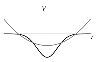
Figure 4: The variational instanton (black) and its approximation by a harmonic potential (grey) (here for $D=1$, $d=4$). Note that the curvature of $V(r)$ is the quadratic term before normal-ordering, whereas in the variational approximation the quadratic term after normal-ordering appears.

The second point is that in the limit when

$$d\,\to\,\infty\quad,\qquad\epsilon\ \text{fixed}$$ (305)

these perturbative terms are subdominant (of order $1/d$) with respect to the leading term obtained by replacing $V$ by the trial harmonic potential ${m^{2}\over 2}:\!\mathsf{r}^{2}\!:_{m}$. This is seen by rescaling $\mathsf{x}$ and $\mathsf{r}$ in units of the variational mass $m$ (as described in detail in Appendix G), so that $m\to 1$, and the propagator $G_{m}(\mathsf{x})$ becomes $G(\mathsf{x})=G_{1}(x)$

$$G_{m}(\mathsf{x})\to G(\mathsf{x})=G_{m=1}(\mathsf{x})=(2\pi)^{-{D\over 2}}K_{{D-2\over 2}}(|\mathsf{x}|)$$ (306)

and the tadpole amplitude $G_{m}$ becomes

$$G_{m}\to c_{0}(D)=G(0)=(4\pi)^{-D/2}\Gamma\left({2-D\over 2}\right)\,\simeq\,{1\over 4\pi}{d\over 4-\epsilon}\qquad\text{when}\quad d\to\infty\ ,\ \ \epsilon\ \text{fixed}\ .$$ (307)

$c_{0}(D)$ is noted $\mathbb{C}$ in DavidWiese1998 . When we shall not deal with the explicit dependence on $D$ of $c_{0}(D)$ we shall denote it simply by $c_{0}$.

The variational instanton potential becomes (see Appendix G)

$${V_{\mathrm{var}}^{\mathrm{inst}}}(\mathsf{r})\ =\ -2c_{0}\,{1\mathrm{l}}\,+\,{1\over 2}\,{:\!\mathsf{r}^{2}\!:}\,+\,U(\mathsf{r})\quad,\quad U(\mathsf{r})\,=\,-\,2c_{0}\sum_{n=2}^{\infty}{1\over n!}\left({-1\over 4c_{0}}\right)^{n}\,{:\!\left(\mathsf{r}^{2}\right)^{n}\!:}\ ,$$ (308)

where the normal product $:\cdots:$ refers to the normal product with respect to the unit mass $m=1$, i.e. $:\cdots:=:\cdots:_{m=1}$.

Since $c_{0}\sim d$, in perturbation theory, the $2n$-leg vertices carry a weight $d^{1-n}$ and closed loops carry a weight $d$ (summation over bulk space indices). Counting the resulting factors of $d$ for each graph, as in the large-$N$ expansion for vector models, only “cactus diagrams” with tadpoles survive in the large-$d$ limit. However within our normal product scheme, there are no tadpoles. Therefore for any observable at large $d$ we can replace

$$\left<\text{Observable}\right>_{{V_{\mathrm{var}}^{\mathrm{inst}}}}\ =\ \left<\text{Observable}\right>_{m}\,+\,\text{subdominant terms in}\ {1\over d}\ ,$$ (309)

where $\left<\cdots\right>_{m}$ refers to the expectation value with respect to the trial variational action

$$H_{\text{trial}}^{\text{var}}\ =\ \int_{\mathsf{x}}\,{1\over 2}(\nabla\mathsf{r})^{2}+{m^{2}\over 2}\mathsf{r}^{2}\ .$$ (310)

For the same reason, as shown in DavidWiese1998 , at leading order in $1/d$, the variational instanton, solution of

$${V_{\mathrm{var}}^{\mathrm{inst}}}(\mathsf{r})\,+\,\left<\delta^{d}(\mathsf{r}-\mathsf{r}(\mathsf{o}))\right>_{m}=0$$ (311)

is a good approximation for the exact instanton ${V^{\mathrm{inst}}}$, solution of (89):

$${V^{\mathrm{inst}}}(\mathsf{r})\ =\,{V_{\mathrm{var}}^{\mathrm{inst}}}(\mathsf{r})\,\Bigl{(}1+\mathcal{O}(1/d)\Bigr{)}\ .$$ (312)

The first correction of order $1/d$ was computed in DavidWiese1998 . Finally the action for the variational instanton was found to be

$${\mathcal{S}_{\mathrm{var}}^{\mathrm{inst}}}\ =\ m^{D}\,\left(1-{\epsilon\over D}\right)~c_{0}(D)\ .$$ (313)

If we rescale the effective coupling constant $g$ (or equivalently the initial coupling constant $b$) in terms of the variational mass $m$,

$$g\ \to\ m^{D}\,\underline{g}\qquad\text{i.e.}\qquad b\ \to\ m^{D-\epsilon}\,\underline{b}$$ (314)

the instanton action becomes

$$\underline{{\mathcal{S}_{\mathrm{var}}^{\mathrm{inst}}}}\ =\ \left(1-{\epsilon\over D}\right)~c_{0}(D)\ =\ \mathcal{O}(d)\ .$$ (315)

This rescaling will the done at the end, but for the time-being, we keep the explicit mass dependence.

Large-$d$ limit for ${\mathbb{O}}$:

For our problem, in the large-$d$ limit, we shall firstly approximate the Hessian ${\mathbb{O}}$ in the exact instanton background, with kernel ${\mathbb{O}}_{\mathsf{r}_{1}\mathsf{r}_{2}}$ given by (301), by the Hessian ${\mathbb{O}}^{\text{var}}$ in the variational instanton background, with kernel ${\mathbb{O}}_{\mathsf{r}_{1}\mathsf{r}_{2}}^{\text{var}}$ given by

$${\mathbb{O}}_{\mathsf{r}_{1}\mathsf{r}_{2}}^{\text{var}}\ =\ \int_{\mathsf{x}}{\left<\delta^{d}(\mathsf{r}_{1}-\mathsf{r}(\mathsf{o}))\delta^{d}(\mathsf{r}_{2}-\mathsf{r}(\mathsf{x}))\right>}_{V_{\mathrm{var}}^{\mathrm{inst}}}^{\mathrm{conn}}$$ (316)

and then approximate this ${\mathbb{O}}^{\text{var}}$ by its large-$d$ limit ${\mathbb{O}}^{\mathrm{var^{\prime}}}$, with kernel

$${\mathbb{O}}_{\mathsf{r}_{1}\mathsf{r}_{2}}^{\mathrm{var^{\prime}}}\ =\ \int_{\mathsf{x}}{\left<\delta^{d}(\mathsf{r}_{1}-\mathsf{r}(\mathsf{o}))\delta^{d}(\mathsf{r}_{2}-\mathsf{r}(\mathsf{x}))\right>}_{m}^{\mathrm{conn}}\ .$$ (317)

This will be the leading term of a systematic ${1\over d}$ expansion, which can be performed along similar lines as in DavidWiese1998 .

${\mathbb{O}}_{\mathsf{r}_{1}\mathsf{r}_{2}}^{\mathrm{var^{\prime}}}$ can easily be computed, since we now deal with a massive free theory. It is even easier to compute its Fourier transform

$$\begin{split}\widehat{{\mathbb{O}}}_{\mathsf{k}_{1}\mathsf{k}_{2}}^{\mathrm{var^{\prime}}}\,&=\,\int_{\mathsf{r}_{1}}\int_{\mathsf{r}_{2}}\mathrm{e}^{-\mathrm{i}(\mathsf{k}_{1}\mathsf{r}_{1}+\mathsf{k}_{2}\mathsf{r}_{2})}\,{\mathbb{O}}_{\mathsf{r}_{1}\mathsf{r}_{2}}^{\text{var}}\,=\,\int_{\mathsf{x}}{\left<\mathrm{e}^{\mathrm{i}\mathsf{k}_{1}\mathsf{r}(\mathsf{o})}\mathrm{e}^{\mathrm{i}\mathsf{k}_{2}\mathsf{r}(\mathsf{x})}\right>}_{m}-{\left<\mathrm{e}^{\mathrm{i}\mathsf{k}_{1}\mathsf{r}(\mathsf{o})}\right>}_{m}{\left<\mathrm{e}^{\mathrm{i}\mathsf{k}_{2}\mathsf{r}(\mathsf{x})}\right>}_{m}\\ &=\,\mathrm{e}^{-{(\mathsf{k}_{1}^{2}+\mathsf{k}_{2}^{2})}G_{m}(0)/2}\,\int_{\mathsf{x}}\,\left[\mathrm{e}^{-\mathsf{k}_{1}\mathsf{k}_{2}G_{m}(\mathsf{x})}-1\right]\end{split}\ ,$$ (318)

where $G_{m}(\mathsf{x})$ is the massive scalar propagator (138). Note that we have $G_{m}=G_{m}(0)$.

Zero modes:

In order to compute $\mathfrak{D}$, we must take into account the translational zero modes of $\mathcal{S}^{\prime\prime}\!\!={1\mathrm{l}}-{\mathbb{O}}$ and the projector ${\mathbb{P}_{\!\scriptscriptstyle{0}}}$ onto the subspace of zero modes. According to section III.3, these zero modes are the partial derivatives of ${V^{\mathrm{inst}}}$, $V^{\mathrm{zero}}_{a}=\partial_{a}{V^{\mathrm{inst}}}$, and from section IV.1 (see (113)) the projector is

$${\mathbb{P}_{\!\scriptscriptstyle{0}}}_{\mathsf{r}_{1}\mathsf{r}_{2}}=\mathtt{c_{0}}\sum\limits_{a}\partial_{a}{V^{\mathrm{inst}}}(\mathsf{r}_{1})\partial_{a}{V^{\mathrm{inst}}}(\mathsf{r}_{2})$$

(with the constant $\mathtt{c_{0}}$ such that ${\mathbb{P}}^{2}_{0}={\mathbb{P}}_{0}$). In the large-$d$ limit we may approximate ${\mathbb{P}_{\!\scriptscriptstyle{0}}}$ by ${{\mathbb{P}_{\!\scriptscriptstyle{0}}}}^{\mathrm{var}}$

$${\mathbb{P}_{\!\scriptscriptstyle{0}}}^{\mathrm{var}}_{\mathsf{r}_{1}\mathsf{r}_{2}}\ =\ \mathtt{c^{\prime}_{0}}\sum\limits_{a}\partial_{a}{V_{\mathrm{var}}^{\mathrm{inst}}}(\mathsf{r}_{1})\partial_{a}{V_{\mathrm{var}}^{\mathrm{inst}}}(\mathsf{r}_{2})$$ (319)

and since ${V_{\mathrm{var}}^{\mathrm{inst}}}$ is a Gaussian function, ${\mathbb{P}}^{\mathrm{var}}_{0}$ is easily computed. We obtain for its Fourier transform

$$\widehat{{\mathbb{P}_{\!\scriptscriptstyle{0}}}}^{\mathrm{var}}_{\mathsf{k}_{1}\mathsf{k}_{2}}\ =\ -\,{\mathsf{k}_{1}\mathsf{k}_{2}\over m^{2}}\,\mathrm{e}^{-{1\over 2}(\mathsf{k}_{1}^{2}+\mathsf{k}_{2}^{2})G_{m}(0)}\ .$$ (320)

Finally, in the large-order formulas such as (101), to the instanton zero-modes is associated the weight factor

$$\mathfrak{W}\,=\,g^{-{d\over D}}\,\left[{1\over 2\pi d}\int_{\mathsf{r}}(\nabla{V^{\mathrm{inst}}})^{2}\right]^{d/2}\ .$$

In the large-$d$ limit this gives

$$\mathfrak{W}^{\mathrm{var}}\,=\,g^{-{d\over D}}\,\left[{1\over 2\pi d}\int_{\mathsf{r}}(\nabla{V_{\mathrm{var}}^{\mathrm{inst}}})^{2}\right]^{d/2}\,=\,g^{-{d\over D}}\,\left[{m^{2}\over 2\pi}\right]^{d/2}\ =\ \left[{{\overline{g}}^{-{2\over D}}\over 2\pi}\right]^{d/2}$$ (321)

so that

$$\log\left(\mathfrak{W}^{\mathrm{var}}\right)=\mathcal{O}(d)\ .$$

V.3.2 Large-$d$ calculation of $\mathfrak{L}$

Series representation for $\mathfrak{L}$:

We now apply these results to the computation of the determinant, or rather of its logarithm

$$\mathfrak{L}=\log\left({\det}^{\prime}[\mathcal{S}^{\prime\prime}]\right)\ .$$ (322)

Since $\mathcal{S}^{\prime\prime}={1\mathrm{l}}-{\mathbb{O}}$ and since ${\det}^{\prime}$ subtracts the zero modes, we can write

$$\mathfrak{L}=\mbox{tr}\bigl{[}\log\left({1\mathrm{l}}-{\mathbb{Q}}\right)\bigr{]}\quad;\qquad{\mathbb{Q}}\ =\ {\mathbb{O}}-{\mathbb{P}_{\!\scriptscriptstyle{0}}}\ .$$ (323)

Note that $\mathfrak{L}$ has an imaginary part since $\mathcal{S}^{\prime\prime}$ has one negative eigenvalue $\lambda^{-}$. We expand the log as

$$\mathfrak{L}=-\sum_{k=1}^{\infty}{1\over k}\,\mbox{tr}\bigl{[}{\mathbb{Q}}^{k}\bigr{]}\ .$$ (324)

As we shall see, further simplifications occur in the large-$d$ limit. In this limit we can approximate ${\mathbb{Q}}$ by ${\mathbb{Q}}^{\mathrm{var^{\prime}}}$ given by

$${\mathbb{Q}}^{\mathrm{var^{\prime}}}\ =\ {\mathbb{O}}^{\mathrm{var^{\prime}}}-{\mathbb{P}_{\!\scriptscriptstyle{0}}}^{\mathrm{var}}\ ,$$ (325)

where ${\mathbb{O}}^{\mathrm{var^{\prime}}}$ defined by (317) is the Hessian $-\mathcal{E}^{\prime\prime}$ at the variational instanton, computed in the variational approximation, while ${\mathbb{P}_{\!\scriptscriptstyle{0}}}^{\mathrm{var}}$ defined by (320) is the projector on the zero-modes of $\mathcal{S}^{\prime\prime}$ in the variational approximation. Therefore we approximate $\mathfrak{L}$ by

$$\mathfrak{L}^{\mathrm{var^{\prime}}}=-\sum_{k=1}^{\infty}{1\over k}\,\mbox{tr}\Bigl{[}{\bigl{(}{\mathbb{Q}}^{\mathrm{var^{\prime}}}\bigr{)}}^{k}\Bigr{]}\ .$$ (326)

“Beads” and “necklace” diagrammatic representation:

Starting from (318), (320) and using the fact that $\int_{\mathsf{x}}G_{m}(\mathsf{x})=1/m^{2}$, we can write the kernel of ${\mathbb{Q}}^{\mathrm{var^{\prime}}}$ as

$$\widehat{{\mathbb{Q}}}^{\mathrm{var^{\prime}}}_{\mathsf{k}_{1},\mathsf{k}_{2}}=\mathrm{e}^{-{(\mathsf{k}_{1}^{2}+\mathsf{k}_{2}^{2})}G_{m}(0)/2}\int_{\mathsf{x}}\left[\mathrm{e}^{-\mathsf{k}_{1}\mathsf{k}_{2}G_{m}(\mathsf{x})}-1+\mathsf{k}_{1}\mathsf{k}_{2}\,G_{m}(\mathsf{x})\right]\ ,$$ (327)

and expanding in $\mathsf{k}_{1}\mathsf{k}_{2}$, we get a simple diagrammatic representation for $\widehat{{\mathbb{Q}}}^{\mathrm{var^{\prime}}}_{\mathsf{k}_{1},\mathsf{k}_{2}}$ as a sum of “watermelon” diagrams

$$\begin{split}\widehat{{\mathbb{Q}}}^{\mathrm{var^{\prime}}}_{\mathsf{k}_{1},\mathsf{k}_{2}}&=\mathrm{e}^{-{(\mathsf{k}_{1}^{2}+\mathsf{k}_{2}^{2})}G_{m}(0)/2}\,\sum_{n=2}^{\infty}{(-1)^{n}\over n!}\,(\mathsf{k}_{1}\mathsf{k}_{2})^{n}\,\int_{\mathsf{x}}\,G_{m}(\mathsf{x})^{n}\\ &=\ \parbox{227.62204pt}{\includegraphics[width=227.62204pt]{./figures/bubblesum}}\end{split}\ .$$ (328)

Each line represents a propagator $G_{m}$. No internal $\mathcal{M}$ momentum flows in the diagram, the $\mathsf{p}$’s are external momenta relative to the embedding space $\mathbb{R}^{d}$. In this series the term $n=0$ is removed by the fact that ${\mathbb{O}}$ is defined by a connected correlator in (301); while the term $n=1$ is removed by the projector onto the zero modes ${\mathbb{P}_{\!\scriptscriptstyle{0}}}$.

Now we consider the $\mbox{tr}[{({\mathbb{Q}}^{\mathrm{var^{\prime}}})}^{k}]$ in (326). Each trace is given by

$$\mbox{tr}\Bigl{[}{\bigl{(}{\mathbb{Q}}^{\mathrm{var^{\prime}}}\bigr{)}}^{k}\Bigr{]}=\int{\mathrm{d}^{d}\mathsf{k}_{1}\over(2\pi)^{d}}\cdots{\mathrm{d}^{d}\mathsf{k}_{k}\over(2\pi)^{d}}\ \widehat{{\mathbb{Q}}}^{\mathrm{var^{\prime}}}_{\mathsf{k}_{1},\,-\mathsf{k}_{2}}\widehat{{\mathbb{Q}}}^{\mathrm{var^{\prime}}}_{\mathsf{k}_{2},\,-\mathsf{k}_{3}}\cdots\widehat{{\mathbb{Q}}}^{\mathrm{var^{\prime}}}_{\mathsf{k}_{k},\,-\mathsf{k}_{1}}\ .$$ (329)

Thus $\mathfrak{L}^{\mathrm{var^{\prime}}}$ can be represented as a sum over “necklace” diagrams made out of the “beads” of (328). The integration over the $\mathsf{k}$’s can be done explicitly and gives a decomposition of the form

$$\mbox{tr}\Bigl{[}{\bigl{(}{\mathbb{Q}}^{\mathrm{var^{\prime}}}\bigr{)}}^{k}\Bigr{]}=\sum_{n_{1},\dots,n_{k}\geq 2}P_{n_{1},\dots,n_{k}}(d)\ \prod_{i=1}^{k}2m^{2}G_{m}(0){I_{n_{i}}\over 2^{n_{i}}n_{i}!}\quad,\quad I_{n}=\int_{\mathsf{x}}\left[{G_{m}(\mathsf{x})\over G_{m}(0)}\right]^{n}\ ,$$ (330)

where $P_{n_{1},\dots,n_{k}}(d)$ is a polynomial in $d$ (the bulk space dimension), with integer coefficients, given by the average

$$P_{n_{1},\dots,n_{k}}(d)=\overline{(-\mathsf{k}_{1}\mathsf{k}_{2})^{n_{1}}(-\mathsf{k}_{2}\mathsf{k}_{3})^{n_{2}}\cdots(-\mathsf{k}_{k}\mathsf{k}_{1})^{n_{k}}}$$ (331)

with the normalized Gaussian independent variables $\mathsf{k}_{i}\in\mathbb{R}^{d}$, i.e. $\overline{\mathsf{k}_{i}^{a}\mathsf{k}_{j}^{b}}=\delta^{ab}\delta_{ij}$ . The polynomial $P$ can be computed by Wick’s theorem. Typical configurations are:

Note that the first and last points are identified. Let us denote by $N$ the total number of lines $N=\sum n_{i}$ in the diagram. From (331) the $P$’s are non zero if and only if the $n_{i}$’s are either all even, or all odd.

• If $k=1$ this is always true and $P_{n}(d)$ is of degree $n$ in $d$.

• If $k>1$ and the $n_{i}$’s are even, $N\geq 2k$ and the degree of $P(d)$ is $N/2\geq k$.

• If $k>1$ the $n_{i}$’s are odd, $N\geq 3k$ and the degree of $P(d)$ is $1+(N-k)/2>k$.

Large-$d$ power counting:

We now look at the behavior of these terms when $d\to\infty$, $\epsilon$ fixed. First we rescale everything in units of the variational mass $m$,

$$\mathsf{x}\to\mathsf{x}/m\quad,\qquad\mathsf{p}\to\mathsf{p}\,m^{{2-D\over 2}}\quad,\qquad G_{m}(\mathsf{x})\to m^{2-D}G(\mathsf{x})\ ,$$ (332)

that is set the variational mass $m$ to unity in our calculations, since the $\mbox{tr}[{\mathbb{Q}}^{k}]$ are dimensionless quantities. We refer to Appendix G for the details on this rescaling. Then we note that the propagator $G(\mathsf{x})$ for $\mathsf{x}\neq 0$ given by (138) is of order $\mathcal{O}(1)$ when $d\to\infty$

$$G(\mathsf{x})=(2\pi)^{-{D\over 2}}|\mathsf{x}|^{{2-D\over 2}}K_{{D-2\over 2}}(|\mathsf{x}|)\ \to\ {1\over 2\pi}K_{0}(|\mathsf{x}|)\ =\ \mathcal{O}(1)\ ,$$

while $G(0)$ is of order $\mathcal{O}(d)$ since

$$G(0)=(4\pi)^{-{D\over 2}}\Gamma\left({\scriptstyle{2-D\over 2}}\right)\ \to\ {1\over 2\pi}{1\over 2-D}\ \simeq{d\over 4\pi(4-\epsilon)}\ =\ \mathcal{O}(d)\ .$$

Thus the integrals $I_{n}$ given by (330) are of order $d^{-n}$

$$I_{n}=\int_{\mathsf{x}}\left[{G(\mathsf{x})\over G(0)}\right]^{n}=\mathcal{O}(d^{-n})\ ,$$

and the term associated to the $k$-bead necklace $[n_{1},n_{2},\cdots,n_{k}]$ in the decomposition (330) is of order

$$[n_{1},n_{2},\cdots,n_{k}]\ \to\ \mathcal{O}\left({d}^{\text{degree}[P]+k-N}\right)$$

where $N=\sum n_{i}$.

• If $k=1$, we have seen that $\text{degree}[P]=N$, and all the terms are of order $d$. Therefore, if the series over the $n$’s converges (we shall discuss this later)

  $$\mbox{tr}\left[{{\mathbb{Q}}^{\mathrm{var^{\prime}}}}\right]\ =\ \mathcal{O}(d)\ .$$ (333)

• If $k>1$ we have seen that there are two cases. For even necklaces the $n_{i}$’s are all even and $\text{degree}[P]=N/2\geq k$ so we obtain a term of order ${d\,}^{k-{N\over 2}}\leq d^{0}$ We note that the most dominant terms are those with $N=2k$. These are the $[2,2,\cdots,2]$ necklaces whose beads contain 2 links (chains of bubbles).

  (334)

  For odd necklaces, the $n_{i}$’s are all odd and $\text{degree}[P]=1+(N-k)/2>k$, while $N\geq 3k$. This gives a term of order ${d\,}^{1-{{N-k\over 2}}}\leq d^{1-k}\ll 1$. The conclusion is that (as long as we can sum the necklace series) the $k>1$ terms are of order $\mathcal{O}(1)$

  $$k>1\quad\Rightarrow\quad\mbox{tr}\left[\big{(}{{\mathbb{Q}}^{\mathrm{var^{\prime}}}}\big{)}^{k}\right]\ =\mathcal{O}(1)\ ,$$ (335)

  and that the dominant contribution is given by the chain of bubbles.

Final result:

All the $k>1$ terms in (330) are subdominant with respect to the $k=1$ term. In the large-$d$ limit, $\mathfrak{L}$ is of order $\mathcal{O}(d)$ and can be approximated by

$$\mathfrak{L}\ =\ -\,\mbox{tr}\left[{{\mathbb{Q}}^{\mathrm{var^{\prime}}}}\right]\,+\,\mathcal{O}(1)\ .$$ (336)

We shall check this result with explicit calculations. As we shall see, the summation of the necklace series is not completely obvious, and is impaired by the UV divergences of the theory. Let us also note that the imaginary part which comes from the unstable eigenmode of $\mathcal{S}^{\prime\prime}={1\mathrm{l}}-{\mathbb{O}}$ is an effect of order $\mathcal{O}(1)$ (since it is associated with one single eigenvalue).

V.4 Explicit calculations at large $d$

V.4.1 $\mbox{tr}\!\left[{{\mathbb{Q}}^{\mathrm{var^{\prime}}}}\right]$ and its large-$d$ limit for $\epsilon>0$:

We first consider the leading term $\mbox{tr}\left[{{\mathbb{Q}}^{\mathrm{var^{\prime}}}}\right]$, given by

$$\mbox{tr}\left[{{\mathbb{Q}}^{\mathrm{var^{\prime}}}}\right]\ =\ \mbox{tr}\left[{{\mathbb{O}}^{\mathrm{var^{\prime}}}}\right]\ -\ d\$$ (337)

$\mathsf{x}$-integral representation:

$\mbox{tr}\left[{{\mathbb{O}}^{\mathrm{var^{\prime}}}}\right]$ is easily calculated from (318) and (329).

$$\begin{split}\mbox{tr}\left[{{\mathbb{O}}^{\mathrm{var^{\prime}}}}\right]\ &=\ \int{\mathrm{d}^{d}\mathsf{k}\over(2\pi)^{d}}\,{{\mathbb{O}}^{\mathrm{var^{\prime}}}_{\mathsf{k},-\mathsf{k}}}\ =\ \int{\mathrm{d}^{d}\mathsf{k}\over(2\pi)^{d}}\mathrm{e}^{-\mathsf{k}^{2}G_{m}(0)}\,\int_{\mathsf{x}}\,\left[\mathrm{e}^{\mathsf{k}^{2}G_{m}(\mathsf{x})}-1\right]\end{split}$$

The $\mathsf{k}$-integration is Gaussian and gives, using the equation for $m$ (302)

$$\begin{split}\mbox{tr}\left[{{\mathbb{O}}^{\mathrm{var^{\prime}}}}\right]\ &=\ 2\,m^{2}\,G_{m}(0)\int_{\mathsf{x}}\left(\left[1-{G_{m}(\mathsf{x})\over G_{m}(0)}\right]^{-{d\over 2}}-1\right)\end{split}$$ (338)

Since $\mbox{tr}\left[{{\mathbb{O}}^{\mathrm{var^{\prime}}}}\right]$ is dimensionless we can set the variational mass $m$ to unity $m=1$, in the r.h.s. of (338) (see Appendix G). Using the explicit form (306) for the propagator $G(x)$ and integrating over the $\mathsf{x}$ angular variables via $\int\mathrm{d}^{D}\mathsf{x}=\mathcal{S}_{D}\int_{0}^{\infty}\mathrm{d}x\,x^{D-1}$ with $x=|x|$ we obtain

$$\begin{split}\mbox{tr}\left[{{\mathbb{O}}^{\mathrm{var^{\prime}}}}\right]\ &=\ 2^{2-D}{\Gamma\left({2-D\over 2}\right)\over\Gamma\left({D\over 2}\right)}\int_{0}^{\infty}\mathrm{d}x\,x^{D-1}\,\left(\left[1-2\left[{x\over 2}\right]^{{2-D\over 2}}{K_{{D-2\over 2}}(x)\over\Gamma\left({2-D\over 2}\right)}\right]^{-{d\over 2}}-1\right)\end{split}\ .$$ (339)

Let us first consider this integral for finite (but a priori large) $d$, and study its convergence.

IR convergence:

At large $\mathsf{x}$ the integral is convergent. Indeed the massive propagator is exponentially decreasing as $G(\mathsf{x})\simeq\exp(-|\mathsf{x}|)$. For finite $d$, and thanks to the $-1$ that comes from the subtraction of the disconnected part, the integrand in (338) is also exponentially decreasing at large $\mathsf{x}$.

UV divergences:

The small-$\mathsf{x}$ behavior of the integral (338) has in fact already been studied in Sect.(IV.3). It was shown that this behavior is governed by the MOPE (155) and is related to the UV divergences at one loop of the model. The integrand in (339) behaves as $\int_{0}^{\cdots}\mathrm{d}x\,x^{\epsilon-D-1}\,\mathtt{C_{0}}$ with $\mathtt{C_{0}}$ given by (190). We thus recover the expected UV divergence at $\epsilon\leq D$, which is proportional to the insertion of the operator ${1\mathrm{l}}$. This UV divergence appears in the series representation (330) of $\mbox{tr}\left[{{\mathbb{O}}^{\mathrm{var^{\prime}}}}\right]$ as the onset of the nonsumability of the series. Indeed, this series is

$$\mbox{tr}\left[{{\mathbb{O}}^{\mathrm{var^{\prime}}}}\right]=2G(0)\sum_{n=1}^{\infty}{P_{n}(d)\over{{2}^{n}}n!}I_{n}\quad\text{with}\quad P_{n}=d(d+2)\cdots(d+2n-2)\ ,$$ (340)

and $I_{n}=\int_{\mathsf{x}}[G(x)/G(0)]^{n}\sim\ n^{-{D\over 2-D}}$ at large $n$. It is easy to check that the series (340) behaves as $\sum_{n}n^{-1+{d\over 2}-{D\over 2-d}}$ and is convergent only if $\epsilon>D$.

Since the model is defined for $\epsilon<D$ by dimensional regularization, the analytic continuation of the integral (338) is its finite part (in the sense of distribution theory). Therefore $\mbox{tr}\left[{{\mathbb{O}}^{\mathrm{var^{\prime}}}}\right]$ is defined for $\epsilon>0$ by

$$\begin{split}\mbox{tr}\left[{{\mathbb{O}}^{\mathrm{var^{\prime}}}}\right]\ &=\ 2\,G(0)\,\times\ \mbox{f.p.}\int_{\mathsf{x}}\left(\left[1-{G(\mathsf{x})\over G(0)}\right]^{-{d\over 2}}-1\right)\ ,\end{split}$$ (341)

or equivalently by the resummation of the series (340) by a zeta-function prescription.

For $\epsilon=0$ the integral has another UV divergence, which is canceled by the $(\nabla\mathsf{r})^{2}$ counterterm of the renormalized theory. We shall discuss this point later.

large-$d$ limit:

We can now take the limit of (340) when

$$d\to\infty\quad,\qquad\epsilon>0\quad\text{fixed}\ .$$

Since in this limit

$$G(\mathsf{x})\to{1\over 2\pi}K_{0}(|\mathsf{x}|)\quad,\qquad G(0)\to\ {1\over 4\pi}{d\over 4-\epsilon}$$

we obtain

$$\begin{split}\mbox{tr}\left[{{\mathbb{O}}^{\mathrm{var^{\prime}}}}\right]\ &=\ d\,{1\over 4-\epsilon}\ \mbox{f.p.}\int_{0}^{\infty}\hskip-4.30554pt\mathrm{d}x\,x\,\left[\mathrm{e}^{{(4-\epsilon)}K_{0}(x)}-1\right]\ +\ \mathcal{O}(1)\end{split}\ .$$ (342)

From the short distance behavior of the 2-dimensional propagator $K_{0}(x)\simeq\log(1/x)$, the last integral is

$$T_{1}(\epsilon)=\text{f.p.}\int_{0}^{\infty}\hskip-4.30554pt\mathrm{d}x\,x\,\left[\mathrm{e}^{{(4-\epsilon)}K_{0}(x)}-1\right]=\ \int_{0}^{\infty}\hskip-4.30554pt\mathrm{d}x\,x\,\left[\mathrm{e}^{{(4-\epsilon)}K_{0}(x)}-1-x^{-4+{\epsilon}}\right]$$

and is UV finite for $0<\epsilon<2$. Thus we recover that $\mbox{tr}\left[{{\mathbb{O}}^{\mathrm{var^{\prime}}}}\right]=\mathcal{O}(d)$ in this case.

$T_{1}(\epsilon)$ has a single pole at $\epsilon=2$, as expected. It is UV divergent when $\epsilon\to 0$. This will be studied later.

V.4.2 $\mbox{tr}\!\left[\left({{\mathbb{Q}}^{\mathrm{var^{\prime}}}}\right)^{2}\right]$ and its large-$d$ limit for $\epsilon>0$:

We now perform the same analysis for $\mbox{tr}\left[{\mathbb{Q}}^{2}\right]$. We have, using (302)

$$\begin{split}&\mbox{tr}\!\left[\left({{\mathbb{Q}}^{\mathrm{var^{\prime}}}}\right)^{2}\right]=\int{\mathrm{d}^{d}\mathsf{k}_{1}\over(2\pi)^{d}}{\mathrm{d}^{d}\mathsf{k}_{2}\over(2\pi)^{d}}\,\widehat{{\mathbb{Q}}}^{\mathrm{var^{\prime}}}_{\mathsf{k}_{1},-\mathsf{k}_{2}}\widehat{{\mathbb{Q}}}^{\mathrm{var^{\prime}}}_{\mathsf{k}_{2},-\mathsf{k}_{1}}=\int{\mathrm{d}^{d}\mathsf{k}_{1}\over(2\pi)^{d}}{\mathrm{d}^{d}\mathsf{k}_{2}\over(2\pi)^{d}}\,\mathrm{e}^{-(\mathsf{k}_{1}^{2}+\mathsf{k}_{2}^{2})G_{m}(0)}\ \times\\ &\qquad\qquad\qquad\quad\times\int_{\mathsf{x}_{1}}\int_{\mathsf{x}_{2}}\left[\mathrm{e}^{-\mathsf{k}_{1}\mathsf{k}_{2}G_{m}(\mathsf{x}_{1})}-1+\mathsf{k}_{1}\mathsf{k}_{2}G_{m}(\mathsf{x}_{1})\right]\left[\mathrm{e}^{-\mathsf{k}_{1}\mathsf{k}_{2}G_{m}(\mathsf{x}_{2})}-1+\mathsf{k}_{1}\mathsf{k}_{2}G_{m}(\mathsf{x}_{2})\right]\end{split}$$ (343)

Setting $m=1$ and performing the $\mathsf{k}$ integrations we get

$$\begin{split}&4\,G(0)^{2}\int\limits_{\mathsf{x}_{1}}\int\limits_{\mathsf{x}_{2}}\Bigg{\{}{\left[1-\left[{G(\mathsf{x}_{1})+G(\mathsf{x}_{2})\over 2G(0)}\right]^{2}\right]^{-{d\over 2}}\hskip-4.30554pt-\left[1-\left[{G(\mathsf{x}_{1})\over 2G(0)}\right]^{2}\right]^{-{d\over 2}}\hskip-4.30554pt-\left[1-\left[{G(\mathsf{x}_{2})\over 2G(0)}\right]^{2}\right]^{-{d\over 2}}\hskip-4.30554pt+1}\\ &\qquad\qquad\qquad\qquad{-\ d\,{G(\mathsf{x}_{1})G(\mathsf{x}_{2})\over 4\,G(0)^{2}}\,\left[\left[1-\left[{G(\mathsf{x}_{1})\over 2G(0)}\right]^{2}\right]^{-{d\over 2}-1}+\left[1-\left[{G(\mathsf{x}_{2})\over 2G(0)}\right]^{2}\right]^{-{d\over 2}-1}-1\right]}\Bigg{\}}\end{split}$$ (344)

This integral is IR and UV finite as long as $\epsilon>0$. When $\epsilon=0$ we recover the UV divergence when both $\mathsf{x}_{1}$ and $\mathsf{x}_{2}\to 0$.

Now in the large-$d$ limit, $\epsilon$ fixed, since $G(0)\sim d$ and $G(x)\sim 1$ we can expand the $\left[\cdots\right]^{-d/2}$ and get

$${3d(d+2)\over 16\,G(0)^{2}}\int_{\mathsf{x}_{1}}\int_{\mathsf{x}_{2}}G(\mathsf{x}_{1})^{2}\,G(\mathsf{x}_{2})^{2}\ +\ \mathcal{O}(d^{-1}) = \frac{3}{16}\left(2D-\epsilon\right)\left(2+D-\epsilon\right)+\ \mathcal{O}(d^{-1})$$ (345)

$$\approx {3}\left(1-{\epsilon\over 4}\right)^{2}\,+\ \mathcal{O}(d^{-1})\$$

This expansion is not valid for $\mathsf{x}_{1}$ and $\mathsf{x}_{2}=0$ when $\epsilon=0$ and this gives the $1/\epsilon$ UV pole (coupling constant renormalization), but this is an effect exponentially small in the large-$d$ limit. We have thus checked the fact that

$$\mbox{tr}\!\left[\left({{\mathbb{Q}}^{\mathrm{var^{\prime}}}}\right)^{2}\right]=\mathcal{O}(1)$$ (346)

V.4.3 $\mbox{tr}\!\left[\left({{\mathbb{Q}}^{\mathrm{var^{\prime}}}}\right)^{k}\right]$ and its large-$d$ limit for $\epsilon>0$:

Calculation of higher powers can be done along the same line. We get

$$\mbox{tr}\!\left[\left({{\mathbb{Q}}^{\mathrm{var^{\prime}}}}\right)^{k}\right]=\left(1-{\epsilon\over 4}\right)^{k}\,+\,\mathcal{O}(d^{-1})\ .$$ (347)

VI $1/d$ corrections to the large $d$ limit

In this section we study the first $1/d$ correction to the variational solution, which was shown to be valid for large $d$, $\epsilon$ being kept fixed.

VI.1 $1/d$ diagrammatic

We first recall in this subsection how is constructed and organized the $1/d$ expansion, following the ideas of our first paper DavidWiese1998 . We have performed the rescaling (332) so that the variational mass $m$ is set to unity. This rescaling is detailled in Appendix G. We denote by $c_{0}$ the normalized tadpole amplitude and the integration measure over $d$-momenta $\mathsf{k}$ is now normalized so that we have

$$m=1\quad,\quad c_{0}=(4\pi)^{-D/2}\Gamma((2-D)/2)=\parbox{28.45274pt}{\includegraphics[width=28.45274pt]{tadpole}}\quad,\quad\int_{\mathsf{k}}\mathrm{e}^{-\mathsf{k}^{2}c_{0}}=2c_{0}$$ (348)

The exact instanton potential is in these units of the form

$${V^{\mathrm{inst}}}(\mathsf{r})=2c_{0}\sum_{n=0}^{\infty}{1\over 2^{n}n!}\left({-1\over 2c_{0}}\right)^{n}\mu_{n}\,{:\!{(\mathsf{r}^{2})}^{n}\!:}\ ,$$ (349)

where now the normal products are defined with respect to the unit variational mass $m=1$, i.e.

$$:\quad:\,=\,:\quad:_{m=1}$$

and the coefficients $\mu_{n}$ are of order $1$ in the large-$d$ limit, and are found to be

$$\mu_{n}=-1+{\delta_{n}\over d}+\mathcal{O}(d^{-2})$$ (350)

in the large-$d$ limit, with $\delta_{n}=\delta_{n}(D,d)$ given by a self-consistent equation that we recall later. We remind the reader that if we set the $\mu_{n}=-1$ we recover the variational instanton ${V_{\mathrm{var}}^{\mathrm{inst}}}$.

$$\begin{matrix}\text{order\ }n&0&1&2&3&4&\cdots\\ &&&&&&\\ 2n-\text{vertex}&\includegraphics[scale={.5}]{0L-vertex}&\includegraphics[scale={.5}]{2L-vertex}&\parbox{42.5pt}{\includegraphics[scale={.5}]{4L-vertex}}&\parbox{49.5pt}{\includegraphics[scale={.5}]{6L-vertex}}&\parbox{47.0pt}{\includegraphics[scale={.5}]{8L-vertex}}&\cdots\\ &&&&&&\\ \text{couplings}&c_{0}(d/2-2\mu_{0})&\mu_{1}+1&{-\mu_{2}\over 2c_{0}}&{\mu_{3}\over(2c_{0})^{2}}&{-\mu_{4}\over(2c_{0})^{3}}&\cdots\\ &&&&&&\\ \mathcal{O}(1/d)&c_{0}(d/2+2-{2\delta_{1}/d})&{\delta_{1}\over d}&{1\over 2c_{0}}&{-1\over(2c_{0})^{2}}&{-1\over(2c_{0})^{3}}&\cdots\end{matrix}$$

Figure 5: Self energy ($n=0$), mass ($n=1$) and interaction ($n\geq 2$) vertices and couplings in the $U$ expansion (the symmetry factors $1/(2^{n}n!)$ for the vertices are not written).

The perturbative diagrammatics is obtained by writing

$${V^{\mathrm{inst}}}(\mathsf{r})={1\over 2}\mathsf{r}^{2}+U(\mathsf{r})$$ (351)

and treating $U$ as a perturbation. The corresponding $2n$-vertices and couplings are schematically depicted on Fig. 5. The last line represents the couplings which have to be kept at order $1/d$. The propagator is the usual bosonic propagator with unit mass $G(x)$. The one-loop tadpole graph is absent since it is subtracted by the normal-product prescription. The external $\mathsf{r}$-space indices $a=1,\cdots,d$ flow along the closed lines as in a standard O($n$) model.

$\parbox{74.0pt}{\includegraphics[scale={.5}]{bbline0}}=1+\parbox{28.5pt}{\includegraphics[scale={.5}]{onebubble}}+\parbox{58.0pt}{\includegraphics[scale={.5}]{twobubble}}+\parbox{87.0pt}{\includegraphics[scale={.5}]{threebubble}}+\cdots$

Figure 6: The chains of bubbles in the large-$d$ expansion

It was shown in DavidWiese1998 that the diagrams can be reorganized in a $1/d$ expansion by summing all the chains of bubbles, as depicted in Fig.6. More precisely, the propagator for the chain is given by the geometric series (in Fourier transform w.r.t. $\mathsf{x}$ space)

$$\begin{split}\parbox{74.0pt}{\includegraphics[scale={.5}]{bbline0}}=H(\mathsf{p})=\left[1+\mu_{2}{d\over 4c_{0}}B(\mathsf{p})\right]^{-1}\ ,\end{split}$$ (352)

$\mathsf{p}$ being the $D$-momentum flowing through the chain, and $B(\mathsf{p})$ the bubble amplitude (one-loop diagram)

$$\begin{split}{\parbox{28.5pt}{\includegraphics[scale={.5}]{onebubble}}}=B(\mathsf{p})=&\int_{\mathsf{p}}\mathrm{e}^{\mathrm{i}\mathsf{p}\mathsf{x}}\,G(\mathsf{x})^{2}\\ &={1\over\pi}{\mathrm{arcth}\left(p/\sqrt{4+p^{2}}\right)\over p\sqrt{4+p^{2}}}=\frac{1}{\pi}\frac{\mbox{arcsinh}\left(p/2\right)}{p\sqrt{4+p^{2}}}\qquad\text{when}\quad D=2\end{split}$$ (353)

For zero momentum, we have

$$B(0)=\frac{2-D}{2}c_{0}\ .$$ (354)

In practice we also have to consider the chains with $n\geq 1$ or $n\geq 2$ bubbles. They are depicted as follows, with the associated amplitude $H^{(1)}(\mathsf{p})$ and $H^{(2)}(\mathsf{p})$

$$\begin{split}\parbox{74.0pt}{\includegraphics[scale={.5}]{bbline1}}&=\parbox{28.5pt}{\includegraphics[scale={.5}]{onebubble}}+\parbox{58.0pt}{\includegraphics[scale={.5}]{twobubble}}+\parbox{87.0pt}{\includegraphics[scale={.5}]{threebubble}}+\cdots\\ &=H^{(1)}(\mathsf{p})=\left[1+\mu_{2}{d\over 4c_{0}}B(\mathsf{p})\right]^{-1}-1\end{split}$$ (355)

$$\begin{split}\parbox{74.0pt}{\includegraphics[scale={.5}]{bbline2}}&=\parbox{58.0pt}{\includegraphics[scale={.5}]{twobubble}}+\parbox{87.0pt}{\includegraphics[scale={.5}]{threebubble}}+\cdots\\ &=H^{(2)}(\mathsf{p})=\left[1+\mu_{2}{d\over 4c_{0}}B(\mathsf{p})\right]^{-1}-1+\mu_{2}{d\over 4c_{0}}B(\mathsf{p})\end{split}$$ (356)

At the diagrammatic level this reorganisation of perturbation theory is very similar to what is done in the $1/N$ expansion for the (linear or non-linear) sigma models, where the bubble chain is the propagator for an auxiliary $\sigma$ field, and the interaction involves only $\mathsf{r}\mathsf{r}\sigma$ and $\sigma^{k}$ ($k\geq 3$) terms. The analytic structure of the perturbation theory is nevertheless quite different, in particular for the UV and IR divergences of the theory, as already discussed in DavidWiese1998 , and as we shall see below.

$$\begin{matrix}\text{vertex}\quad&\quad\includegraphics[scale={.5}]{2L-vertex}\quad&\quad\parbox{58.5pt}{\includegraphics[scale={.5}]{2L-B-vertex}}\quad&\quad\parbox{56.0pt}{\includegraphics[scale={.5}]{3-B-vertex}}\quad&\quad\parbox{42.5pt}{\includegraphics[scale={.5}]{4-B-vertex}}\quad&\quad\cdots\\ \quad&\quad&&&&\\ \text{coupling}\quad&\quad\mu_{1}+1&\sqrt{{-\mu_{2}\over 2c_{0}}}&{1\over\sqrt{2c_{0}}}{\mu_{3}\over(-\mu_{2})^{3/2}}&{1\over 2c_{0}}{-\mu_{4}\over(-\mu_{2})^{2}}&\quad\cdots\\ \quad&\quad&&&&\\ \text{coupling at order}\ {1\over d}\quad&{\delta_{1}\over d}&{1\over\sqrt{2c_{0}}}&-{1\over\sqrt{2c_{0}}}&{1\over 2c_{0}}&\end{matrix}$$

Figure 7: The vertices contributing to $-V^{\mathrm{inst}}(r)$ and their couplings in the large-$d$-reorganized perturbative expansion.

After this resummation the new vertices with their couplings are depicted in Fig.7. The crucial point is that in the limit $d\to\infty$, $\epsilon$ fixed, since $D\to 2$ the tadpole coefficient $c_{0}$ diverges as $d$ so that

$$\mu_{2}{d\over 2c_{0}}\ \to\ -8\pi\left(1-{\epsilon\over 4}\right)\ =\ \mathcal{O}(1)$$ (357)

and the bubble propagator $H(\mathsf{p})$ is of order $\mathcal{O}(1)$, while the vertices are of order $1/\sqrt{d}$, $1/d$, etc. It was shown in DavidWiese1998 that only a finite number of diagrams contribute to a given order in $1/d$, and explicit calculations where done at the first non-trivial order.

With these notations we have found in DavidWiese1998 that at order $1/d$ the following diagrams contribute to the expectation value of the exponential (or vertex) operator

$${\langle\mathrm{e}^{\mathrm{i}\mathsf{k}\mathsf{r}(0)}\rangle}_{V}=\mathrm{e}^{-{\mathsf{k}^{2}\over 2}c_{0}}\ \left[1\,-{\mathsf{k}^{2}}\left(\parbox{28.45274pt}{\includegraphics[width=28.45274pt]{graph-1}}+\parbox{28.45274pt}{\includegraphics[width=28.45274pt]{graph-4}}+\parbox{28.45274pt}{\includegraphics[width=28.45274pt]{graph-2}}+\parbox{28.45274pt}{\includegraphics[width=28.45274pt]{graph-3}}+\parbox{28.45274pt}{\includegraphics[width=28.45274pt]{graph-5}}\right)+{(\mathsf{k}^{2})}^{2}\ \parbox{28.45274pt}{\includegraphics[width=28.45274pt]{graph-6}}\right]$$ (358)

The symmetry factors of the diagrams are not written, they are respectively $1/2$, $1/4$, $1/2$, $1/4$, $1/4$ and $1/8$ for the diagrams in (358). No $\mathsf{r}$-space indices flow through the unclosed line diagram is (taking into account the couplings and the symmetry factors)

$$\parbox{28.45274pt}{\includegraphics[width=28.45274pt]{graph-1}}\ =\ {1\over 2}\,({1+\mu_{1}})\,\int_{\mathsf{x}}G(\mathsf{x})^{2}\,=\ {2-D\over 4}(1+\mu_{1})c_{0}$$

Similarly for the last diagram

$$\parbox{28.45274pt}{\includegraphics[width=28.45274pt]{graph-6}}\ =\ {1\over 8}{-\mu_{2}\over 2c_{0}}\,\,\int_{\mathsf{x}}\int_{\mathsf{y}}G(\mathsf{x})^{2}G(\mathsf{y})^{2}H(\mathsf{x}-\mathsf{y})\,$$

The exact instanton saddle-point equation, which is (once again)

$$\widehat{V}(\mathsf{k})\,+\,{\langle\mathrm{e}^{\mathrm{i}\mathsf{k}\mathsf{r}(0)}\rangle}_{V}\ =\ 0$$ (359)

fixes the $\mu_{n}$’s. In particular $\mu_{1}$ is given by

$$\mu_{1}=-{1\over d}\int_{\mathsf{k}}\mathsf{k}^{2}\,\widehat{V}(\mathsf{k})\,\mathrm{e}^{-{\mathsf{k}^{2}\over 2}c_{0}}$$ (360)

and using (359) and (358) at order $1/d$ we get the equation for $\mu_{1}$ (i.e. $\delta_{1}$) which reads diagrammatically

$$\includegraphics[scale={.25}]{2L-vertex}+{2c_{0}\over d}\left[-\overline{\mathsf{k}^{4}}\left(\parbox{28.45274pt}{\includegraphics[width=28.45274pt]{graph-1}}+\parbox{28.45274pt}{\includegraphics[width=28.45274pt]{graph-4}}+\parbox{28.45274pt}{\includegraphics[width=28.45274pt]{graph-2}}+\parbox{28.45274pt}{\includegraphics[width=28.45274pt]{graph-3}}+\parbox{28.45274pt}{\includegraphics[width=28.45274pt]{graph-5}}\right)+\overline{{\mathsf{k}^{6}}}\ \parbox{28.45274pt}{\includegraphics[width=28.45274pt]{graph-6}}\right]=0\ ,$$ (361)

where $\overline{\mathsf{k}^{4}}$ and $\overline{\mathsf{k}^{6}}$ mean the average value of $\mathsf{k}^{4}$ and $\mathsf{k}^{6}$ respectively with the Gaussian weight $\mathrm{e}^{-\mathsf{k}^{2}c_{0}}$. Since

$$\overline{\mathsf{k}^{4}}={d(d+2)\over(2c_{0})^{2}}\simeq\left({d\over 2c_{0}}\right)^{2}\quad,\quad\overline{\mathsf{k}^{6}}={d(d+2)(d+4)\over(2c_{0})^{3}}\simeq\left({d\over 2c_{0}}\right)^{3}$$ (362)

are of order $\mathcal{O}(1)$ we recover that $\mu_{1}=-1+\mathcal{O}(1/d)$.

VI.2 The Hessian $\mathbb{O}$

We now show how this method to construct a $1/d$ expansion can be applied to compute the matrix elements of the Hessian $\mathcal{S}^{\prime\prime}$ and of the associated operator ${\mathbb{O}}$. We start from the expression for ${\mathbb{O}}$ in momentum space

$$\widehat{{\mathbb{O}}}_{\mathsf{k}_{1}\mathsf{k}_{2}}=\int_{\mathsf{x}}\left<\mathrm{e}^{\mathrm{i}\mathsf{k}_{1}\mathsf{r}(\mathsf{o})}\mathrm{e}^{\mathrm{i}\mathsf{k}_{2}\mathsf{r}(\mathsf{x})}\right>_{V}^{\mathrm{conn}}=\int_{\mathsf{x}}\left<\mathrm{e}^{\mathrm{i}\mathsf{k}_{1}\mathsf{r}(\mathsf{o})}\mathrm{e}^{\mathrm{i}\mathsf{k}_{2}\mathsf{r}(\mathsf{x})}\right>_{V}-\left<\mathrm{e}^{\mathrm{i}\mathsf{k}_{1}\mathsf{r}(\mathsf{o})}\right>_{V}\left<\mathrm{e}^{\mathrm{i}\mathsf{k}_{2}\mathsf{r}(\mathsf{x})}\right>_{V}$$ (363)

and we use our perturbative rules to expand the e.v. $\left<\cdots\right>_{V}$ in $1/d$.

VI.2.1 ${\mathbb{O}}$ at order $1$:

At leading order $\mathcal{O}(1)$, we get (318) that we can represent as a sum over diagrams with $n\geq 1$ propagators between $\mathsf{o}$ and $\mathsf{x}$, integrated over $\mathsf{x}$

$$\begin{split}\widehat{{\mathbb{O}}}_{\mathsf{k}_{1}\mathsf{k}_{2}}^{(0)}&=\int_{\mathsf{x}}\mathrm{e}^{-(\mathsf{k}_{1}^{2}+\mathsf{k}_{2}^{2})c_{0}/2}\left[\mathrm{e}^{-\mathsf{k}_{1}\mathsf{k}_{2}G(\mathsf{x})}-1\right]\\ &=\sum_{n=1}^{\infty}\mathrm{e}^{-\mathsf{k}_{1}^{2}c_{0}/2}\mathrm{e}^{-\mathsf{k}_{2}^{2}c_{0}/2}(\mathrm{i}\mathsf{k}_{1}\cdot\mathrm{i}\mathsf{k}_{2})^{n}\ \raisebox{-10.76385pt}{\includegraphics[width=56.9055pt]{n-L-0}}=\sum_{n=1}^{\infty}\ \raisebox{-10.76385pt}{\includegraphics[width=56.9055pt]{n-L-00}}\end{split}$$ (364)

where the integration over $\mathsf{x}$ and the symmetry factor $1/n!$ of the graphs are implicit. We have introduced here an additional diagrammatic notation, which will be very convenient in the following discussion.

VI.2.2 A diagrammatic representation for the vertex $\widehat{V}(\mathsf{k})$:

The circles in the last graph are a symbol for the factors which depend respectively on $\mathsf{k}_{1}$ and $\mathsf{k}_{2}$ and are attached to the vertices $\mathsf{o}$ and $\mathsf{x}$. More precisely, the circle represents the exponential $\mathrm{e}^{-\mathsf{k}^{2}c_{0}/2}$ and each line entering into the circle represents an additional (multiplicative) factor $\mathrm{i}\mathsf{k}$, with an external space index $a$ carried by the line. Thus the following picture, a circle with $n$ external lines, represents the factor

$$\raisebox{-10.76385pt}{\includegraphics[scale={.5}]{circle-star}}\ =\ \mathrm{e}^{-\mathsf{k}^{2}c_{0}/2}\,(\mathrm{i}\mathsf{k}^{a_{1}})\cdots(\mathrm{i}\mathsf{k}^{a_{n}})\ .$$ (365)

VI.2.3 ${\mathbb{O}}$ at order $1/d$:

Now we make the perturbative expansion and keep the diagrams which contribute to ${\mathbb{O}}$ at order $\mathcal{O}(1/d)$ only. We find that only (!) 21 different (classes of) diagrams contribute

$$\begin{split}\widehat{{\mathbb{O}}}_{\mathsf{k}_{1},\mathsf{k}_{2}}^{(1)}&=\raisebox{-10.76385pt}{\includegraphics[scale={.33}]{graph-O-1}}+\raisebox{-10.76385pt}{\includegraphics[scale={.33}]{graph-O-3}}+\raisebox{-10.76385pt}{\includegraphics[scale={.33}]{graph-O-4}}+\raisebox{-10.76385pt}{\includegraphics[scale={.33}]{graph-O-5}}+\raisebox{-10.76385pt}{\includegraphics[scale={.33}]{graph-O-2}}+\raisebox{-10.76385pt}{\includegraphics[scale={.33}]{graph-O-6}}\\ &+\raisebox{-10.76385pt}{\includegraphics[scale={.33}]{graph-O-1b}}+\raisebox{-10.76385pt}{\includegraphics[scale={.33}]{graph-O-3b}}+\raisebox{-10.76385pt}{\includegraphics[scale={.33}]{graph-O-4b}}+\raisebox{-10.76385pt}{\includegraphics[scale={.33}]{graph-O-5b}}+\raisebox{-10.76385pt}{\includegraphics[scale={.33}]{graph-O-2b}}+\raisebox{-10.76385pt}{\includegraphics[scale={.33}]{graph-O-6b}}\\ &+\raisebox{-10.76385pt}{\includegraphics[scale={.33}]{graph-O-13}}+\raisebox{-10.76385pt}{\includegraphics[scale={.33}]{graph-O-11}}+\raisebox{-10.76385pt}{\includegraphics[scale={.33}]{graph-O-12}}+\raisebox{-10.76385pt}{\includegraphics[scale={.33}]{graph-O-10}}\\ &+\raisebox{-10.76385pt}{\includegraphics[scale={.33}]{graph-O-14}}+\raisebox{-10.76385pt}{\includegraphics[scale={.33}]{graph-O-15}}+\raisebox{-10.76385pt}{\includegraphics[scale={.33}]{graph-O-16}}+\raisebox{-10.76385pt}{\includegraphics[scale={.33}]{graph-O-17}}+\raisebox{-10.76385pt}{\includegraphics[scale={.33}]{graph-O-17b}}\ .\end{split}$$ (366)

VI.2.4 Diagrammatic for the mass renormalization and $V$:

Moreover, Eq. (361) for the mass renormalization $\mu_{1}$ may be rewritten at order $\mathcal{O}(1/d)$ with our notations as

$$\raisebox{0.0pt}{\includegraphics[scale={.33}]{graph-13a}}\ =\raisebox{-10.76385pt}{\includegraphics[scale={.33}]{graph-12a}}+\raisebox{-10.76385pt}{\includegraphics[scale={.33}]{graph-11a}}+\raisebox{-10.76385pt}{\includegraphics[scale={.33}]{graph-10a}}+\mathcal{O}(1/d^{2})\ .$$ (367)

While Eq.(358) for $V$ reads

$$-\,\widehat{V}(\mathsf{k})=\raisebox{0.0pt}{\includegraphics[scale={.33}]{graph-0a}}+\raisebox{0.0pt}{\includegraphics[scale={.33}]{graph-1a}}+\raisebox{0.0pt}{\includegraphics[scale={.33}]{graph-4a}}+\raisebox{0.0pt}{\includegraphics[scale={.33}]{graph-3a}}+\raisebox{0.0pt}{\includegraphics[scale={.33}]{graph-5a}}+\raisebox{0.0pt}{\includegraphics[scale={.33}]{graph-2a}}+\raisebox{0.0pt}{\includegraphics[scale={.33}]{graph-6a}}+\mathcal{O}(1/d^{2})$$ (368)

Note that in Eq. (366) the first 4 diagrams of lines 1 and 2, and the 4 diagrams of line 3 can be absorbed into a mass shift $m=1\ \to\ m=1-\ \raisebox{0.86108pt}{\includegraphics[scale={.33}]{graph-13a}}$ in the leading contribution represented in (364). The same mass shift absorbs the diagrams 2–5 in Eq.(368) for $V$.

VI.3 The zero-mode projector ${\mathbb{P}_{\!\scriptscriptstyle{0}}}$

We now compute the projector onto the zero-modes

$${\widehat{{\mathbb{P}_{\!\scriptscriptstyle{0}}}}}_{\mathsf{k}_{1}\mathsf{k}_{2}}={\mathrm{i}\mathsf{k}_{1}\widehat{V}(\mathsf{k}_{1})\cdot\mathrm{i}\mathsf{k}_{2}\widehat{V}(\mathsf{k}_{2})\over{1\over d}\int_{\mathsf{k}}\mathsf{k}^{2}\widehat{V}(\mathsf{k})^{2}}$$ (369)

VI.3.1 ${\mathbb{P}_{\!\scriptscriptstyle{0}}}$ at order 1

We have already seen that at leading order in the $1/d$ expansion $\int_{\mathsf{k}}\mathsf{k}^{2}\widehat{V}(\mathsf{k})^{2}=d$ and since $\int_{\mathsf{x}}G(\mathsf{x})=\widehat{G}(0)=\frac{1}{m^{2}}=1$ so that with our diagrammatic notations

$$\widehat{{\mathbb{P}_{\!\scriptscriptstyle{0}}}}_{\mathsf{k}_{1}\mathsf{k}_{2}}^{(0)}=\int_{\mathsf{x}}(-\mathsf{k}_{1}\mathsf{k}_{2})\mathrm{e}^{-{\mathsf{k}_{1}^{2}}c_{0}/2}\mathrm{e}^{-{\mathsf{k}_{2}^{2}}c_{0}/2}G(\mathsf{x})=\ \raisebox{0.0pt}{\includegraphics[scale={.33}]{1-La}}\ .$$ (370)

Thus the projector ${\mathbb{P}_{\!\scriptscriptstyle{0}}}$ subtracts the one-line diagram in ${\mathbb{O}}$ (see Eqs.(327)-(328)).

VI.3.2 ${\mathbb{P}_{\!\scriptscriptstyle{0}}}$ at order $1/d$

We can now compute explicitely the first correction in $1/d$ to ${\mathbb{P}_{\!\scriptscriptstyle{0}}}$, using (368) for $V$. It is easy to see that the numerator in (369) gives all the diagrams in the lines (rows) 1 and 2 of (366) with $n=1$ line between the two points $\mathsf{o}$ and $\mathsf{x}$.

$$\begin{split}(-\mathsf{k}_{1}&\cdot\mathsf{k}_{2})\widehat{V}(\mathsf{k}_{1})\widehat{V}(\mathsf{k}_{2})=\ \raisebox{0.0pt}{\includegraphics[scale={.33}]{1-La}}\ +\\ &\raisebox{0.0pt}{\includegraphics[scale={.33}]{graph-O-1c}}+\raisebox{0.0pt}{\includegraphics[scale={.33}]{graph-O-4c}}+\raisebox{0.0pt}{\includegraphics[scale={.33}]{graph-O-2c}}+\raisebox{0.0pt}{\includegraphics[scale={.33}]{graph-O-3c}}+\raisebox{0.0pt}{\includegraphics[scale={.33}]{graph-O-5c}}+\raisebox{0.0pt}{\includegraphics[scale={.33}]{graph-O-6c}}\\ +&\raisebox{0.0pt}{\includegraphics[scale={.33}]{graph-O-1a}}+\raisebox{0.0pt}{\includegraphics[scale={.33}]{graph-O-4a}}+\raisebox{0.0pt}{\includegraphics[scale={.33}]{graph-O-2a}}+\raisebox{0.0pt}{\includegraphics[scale={.33}]{graph-O-3a}}+\raisebox{0.0pt}{\includegraphics[scale={.33}]{graph-O-5a}}+\raisebox{0.0pt}{\includegraphics[scale={.33}]{graph-O-6a}}\end{split}$$ (371)

The denominator is computed from the explicit form of $V$ given by (367)-(368). In fact it is easy to see, using (358), that

$$\begin{split}{1\over d}\int_{\mathsf{k}}\mathsf{k}^{2}{\widehat{V}(\mathsf{k})}^{2}&=1-2\,{\delta_{1}\over d}+\mathcal{O}(1/d^{2})=1-\raisebox{0.0pt}{\includegraphics[scale={.33}]{graph-13a}}-\raisebox{-10.76385pt}{\includegraphics[scale={.33}]{graph-12a}}-\raisebox{-10.76385pt}{\includegraphics[scale={.33}]{graph-11a}}-\raisebox{-10.76385pt}{\includegraphics[scale={.33}]{graph-10a}}+\mathcal{O}(1/d^{2})\end{split}$$ (372)

and since $\widehat{G}(0)=1$ we can write $\raisebox{-0.86108pt}{\includegraphics[scale={.33}]{1-La}}\times\raisebox{0.86108pt}{\includegraphics[scale={.33}]{graph-13a}}=\raisebox{0.0pt}{\includegraphics[scale={.33}]{graph-13}}$ , etc. We obtain that only (!) 16 diagrams contribute to ${\mathbb{P}_{\!\scriptscriptstyle{0}}}$; the final result is

$$\begin{split}&{\widehat{{\mathbb{P}_{\!\scriptscriptstyle{0}}}}}_{\mathsf{k}_{1}\mathsf{k}_{2}}\ =\ \raisebox{0.0pt}{\includegraphics[scale={.33}]{1-La}}+\raisebox{0.0pt}{\includegraphics[scale={.33}]{graph-13}}+\raisebox{0.0pt}{\includegraphics[scale={.33}]{graph-12}}+\raisebox{0.0pt}{\includegraphics[scale={.33}]{graph-11}}+\raisebox{0.0pt}{\includegraphics[scale={.33}]{graph-10}}\\ &+\raisebox{0.0pt}{\includegraphics[scale={.33}]{graph-O-1c}}+\raisebox{0.0pt}{\includegraphics[scale={.33}]{graph-O-4c}}+\raisebox{0.0pt}{\includegraphics[scale={.33}]{graph-O-2c}}+\raisebox{0.0pt}{\includegraphics[scale={.33}]{graph-O-3c}}+\raisebox{0.0pt}{\includegraphics[scale={.33}]{graph-O-5c}}+\raisebox{0.0pt}{\includegraphics[scale={.33}]{graph-O-6c}}\\ +&\raisebox{0.0pt}{\includegraphics[scale={.33}]{graph-O-1a}}+\raisebox{0.0pt}{\includegraphics[scale={.33}]{graph-O-4a}}+\raisebox{0.0pt}{\includegraphics[scale={.33}]{graph-O-2a}}+\raisebox{0.0pt}{\includegraphics[scale={.33}]{graph-O-3a}}+\raisebox{0.0pt}{\includegraphics[scale={.33}]{graph-O-5a}}+\raisebox{0.0pt}{\includegraphics[scale={.33}]{graph-O-6a}}+\ \mathcal{O}(1/d^{2})\end{split}$$ (373)

We note that the denominator gives all the one-line reducible diagrams (with only a single line joining $\mathsf{o}$ and $\mathsf{x}$) with a tadpole-like graph attached to the line. The diagrams , and although one-line-reducible, are not contained in (373).

VI.3.3 An all order argument relating ${\mathbb{P}_{\!\scriptscriptstyle{0}}}$ with tadpole graphs

A simple general argument shows that the denominator in (369), given at first order by the tadpole diagrams depicted in (372), is given at all orders by the tadpole diagrams with two truncated external legs attached to the same vertex. In diagrammatic language we shall show that

$$1-\raisebox{0.0pt}{\includegraphics[scale={.5}]{tadpole-0}}-\raisebox{0.0pt}{\includegraphics[scale={.5}]{tadpole-2}}-\raisebox{0.0pt}{\includegraphics[scale={.5}]{tadpole-4}}-\ \cdots\ =\ {1\over d}\int_{\mathsf{k}}\,\mathsf{k}^{2}\,\widehat{V}(\mathsf{k})^{2}$$ (374)

The l.h.s. of (374) is nothing but

$$1-\raisebox{0.0pt}{\includegraphics[scale={.33}]{tadpole-0}}-\raisebox{0.0pt}{\includegraphics[scale={.33}]{tadpole-2}}-\raisebox{0.0pt}{\includegraphics[scale={.33}]{tadpole-4}}-\ \cdots\ =\ {1\over d}{\left<V^{\prime\prime}\bigl{(}\mathsf{r}(\mathsf{o})\bigr{)}\right>}_{V}\qquad\text{with}\qquad V^{\prime\prime}(\mathsf{r})=\sum_{a}{\partial^{2}V(\mathsf{r})\over\partial\mathsf{r}^{a}\partial\mathsf{r}^{a}}$$ (375)

(the two $\mathsf{r}$ derivatives pick two legs out of the vertex $V(\mathsf{r})$). We can rewrite it as

$$V^{\prime\prime}\bigl{(}\mathsf{r}(\mathsf{o})\bigr{)}=\int_{\mathsf{r}}V^{\prime\prime}(\mathsf{r})\,\delta\bigl{(}(\mathsf{r}-\mathsf{r}(\mathsf{o})\bigr{)}=\ \int_{\mathsf{k}}(-\mathsf{k}^{2})\,\widehat{V}(\mathsf{k})\,\mathrm{e}^{\mathrm{i}\mathsf{k}\mathsf{r}(\mathsf{o})}$$ (376)

and using the exact equation (359) for the instanton potential, we get

$${\left<V^{\prime\prime}\bigl{(}\mathsf{r}(\mathsf{o})\bigr{)}\right>}_{V}\ =\ \int_{\mathsf{k}}(-\mathsf{k}^{2})\,\widehat{V}(\mathsf{k})\,\left<\mathrm{e}^{\mathrm{i}\mathsf{k}\mathsf{r}(\mathsf{o})}\right>_{V}\ =\ \int_{\mathsf{k}}\,\mathsf{k}^{2}\,\widehat{V}(\mathsf{k})^{2}$$ (377)

Q.E.D.

(374) implies that ${\mathbb{P}_{\!\scriptscriptstyle{0}}}$ will contain all the tadpole chains with tadpole graphs attached at the $\mathsf{o}$ and $\mathsf{x}$ end-points, of the form

$${\mathbb{P}_{\!\scriptscriptstyle{0}}}\ =\ \raisebox{0.0pt}{\includegraphics[scale={.33}]{tadpole-all-ext}}$$ (378)

VI.4 Final result for ${\mathbb{Q}}={\mathbb{O}}-{\mathbb{P}_{\!\scriptscriptstyle{0}}}$

As a consequence the subtracted operator ${\mathbb{Q}}={\mathbb{O}}-{\mathbb{P}_{\!\scriptscriptstyle{0}}}$ is given at order $\mathcal{O}(1/d)$ by the same diagrams as those depicted in Eq.(366) for ${\mathbb{O}}$, with the simple restriction that the diagrams in the first two lines of (366) must have at least 2 lines joining the two end-points ($n\geq 2$), and that the diagrams in the third line must have at least one non-dressed line joining the two end-points ($n\geq 1$), while for the diagrams in the fourth line, there is no additional restriction (no constraints on the number $n$ of simple lines, $n\geq 0$). Using equation (367) for $\mu_{1}$ we can rewrite it as a sum over only 12 graphs (instead of 21!)

$$\begin{split}\widehat{{\mathbb{Q}}}^{(1)}_{\mathsf{k}_{1},\mathsf{k}_{2}}&=2\raisebox{-10.76385pt}{\includegraphics[scale={.33}]{graph-O-1e}}+\raisebox{-10.76385pt}{\includegraphics[scale={.33}]{graph-O-2e}}+\raisebox{-10.76385pt}{\includegraphics[scale={.33}]{graph-O-6e}}+2\,\raisebox{-10.76385pt}{\includegraphics[scale={.33}]{graph-O-1f}}+\raisebox{-10.76385pt}{\includegraphics[scale={.33}]{graph-O-2f}}+\raisebox{-10.76385pt}{\includegraphics[scale={.33}]{graph-O-6f}}\\ &\hskip-20.00003pt+2\,\raisebox{-10.76385pt}{\includegraphics[scale={.33}]{graph-O-13b}}+\raisebox{-10.76385pt}{\includegraphics[scale={.33}]{graph-O-14}}+\raisebox{-10.76385pt}{\includegraphics[scale={.33}]{graph-O-15}}+\raisebox{-10.76385pt}{\includegraphics[scale={.33}]{graph-O-16}}+\raisebox{-10.76385pt}{\includegraphics[scale={.33}]{graph-O-17}}+\raisebox{-10.76385pt}{\includegraphics[scale={.33}]{graph-O-17b}}\ .\end{split}$$ (379)

VI.5 The determinant $\mathfrak{D}$

We now compute the $\log$ of the determinant of instanton fluctuations

$$\mathfrak{L}=\log(\mathfrak{D})=\mbox{tr}\log({1\mathrm{l}}-{\mathbb{Q}})=-\sum_{k=1}^{\infty}~{1\over k}\,\mbox{tr}({\mathbb{Q}}^{k})$$ (380)

VI.5.1 Diagrammatic representation of the trace

With our rescalings (see Appendix G) each trace still reads

$$\mathfrak{T}_{k}=\mbox{tr}({\mathbb{Q}}^{k})=\int_{\mathsf{k}_{1}}\cdots\int_{\mathsf{k}_{k}}\widehat{{\mathbb{Q}}}_{\mathsf{k}_{1},-\mathsf{k}_{2}}\widehat{{\mathbb{Q}}}_{\mathsf{k}_{2},-\mathsf{k}_{3}}\cdots\widehat{{\mathbb{Q}}}_{\mathsf{k}_{k},-\mathsf{k}_{1}}$$ (381)

and with the representation for the kernel ${\mathbb{Q}}$, we have to compute integrals over $\mathsf{k}$ of the form,

$$\int_{\mathsf{k}}\mathrm{e}^{-\mathsf{k}^{2}c_{0}}(-\mathrm{i}\mathsf{k}^{a_{1}})\cdots(-\mathrm{i}\mathsf{k}^{a_{m}})\,(\mathrm{i}\mathsf{k}^{b_{1}})\cdots(\mathrm{i}\mathsf{k}^{b_{n}})\ =\ (-1)^{{m-n\over 2}}(2c_{0})^{1-{m+n\over 2}}\,\sum_{\mathrm{pairing}}\delta^{..}\cdots\delta^{..}\ .$$ (382)

Using Wick’s theorem we can represent each term by pairing of lines between the left ${\mathbb{Q}}$ and the right ${\mathbb{Q}}$, as already discussed when we introduced the diagrammatic necklace representation for $\mathfrak{L}$. This is depicted below

$$\raisebox{-4.30554pt}{\includegraphics[scale={.5}]{circle-star-2}}=\mbox{\scriptsize$m$ lines entering}\left\{\raisebox{-4.30554pt}{\includegraphics[scale={.5}]{circle-star-2}}\right\}\mbox{\scriptsize$n$ lines exiting}$$ (383)

$$\int_{\mathsf{k}}\raisebox{-4.30554pt}{\includegraphics[scale={.5}]{circle-star-2}}=(-1)^{{m-n\over 2}}(2c_{0})^{1-{m+n\over 2}}\raisebox{-8.61108pt}{\includegraphics[scale={.5}]{circle-star-3}}\ .$$ (384)

For instance for $m=n=2$

$$\raisebox{-8.61108pt}{\includegraphics[scale={.5}]{circle-star-22}}=\raisebox{-8.61108pt}{\includegraphics[scale={.5}]{circle-star-22a}}+\raisebox{-8.61108pt}{\includegraphics[scale={.5}]{circle-star-22b}}+\raisebox{-8.61108pt}{\includegraphics[scale={.5}]{circle-star-22c}}$$ (385)

and for $m=3$, $n=1$

$$\raisebox{-8.61108pt}{\includegraphics[scale={.5}]{circle-star-31}}=\raisebox{-8.61108pt}{\includegraphics[scale={.5}]{circle-star-31a}}+\raisebox{-8.61108pt}{\includegraphics[scale={.5}]{circle-star-31b}}+\raisebox{-8.61108pt}{\includegraphics[scale={.5}]{circle-star-31c}}\ .$$ (386)

The vertical dotted line indicates that no $\mathcal{M}$-momenta $\mathsf{p}$ flows through the vertex, since each ${\mathbb{Q}}$ is attached to a different replica of the manifold $\mathcal{M}$. With these graphical notations, if we represent the kernel ${\mathbb{Q}}$ by the “bead”

$${\mathbb{Q}}\ =\ \raisebox{-10.76385pt}{\includegraphics[scale={.5}]{Q-graph-a}}$$ (387)

$\mbox{tr}[{\mathbb{Q}}^{k}]$ is represented by the k-bead necklace (with periodic boundary condition between the left and right dashed vertical lines)

$$\mbox{tr}[{\mathbb{Q}}]\,=\,\raisebox{-6.45831pt}{\includegraphics[scale={.4}]{Q-graph}}\quad,\quad\mbox{tr}[{\mathbb{Q}}^{2}]\,=\,\raisebox{-6.45831pt}{\includegraphics[scale={.4}]{Q2-graph}}\quad,\quad\mbox{tr}[{\mathbb{Q}}^{k}]\,=\,\raisebox{-6.45831pt}{\includegraphics[scale={.4}]{Qn-graph}}\ .$$ (388)

VI.5.2 $\mbox{tr}\left[{\mathbb{Q}}\right]$

We first consider the term $k=1$. We have already seen that at leading order in $1/d$

$$\mbox{tr}\left[{\mathbb{Q}}^{(0)}\right]\ =\ \int_{\mathsf{k}}\widehat{{\mathbb{Q}}}_{\mathsf{k},-\mathsf{k}}^{(0)}\ =\ \int_{\mathsf{k}}\int_{\mathsf{x}}\mathrm{e}^{-\mathsf{k}^{2}c_{0}}\left(\mathrm{e}^{\mathsf{k}^{2}G(\mathsf{x})}-1-\mathsf{k}^{2}G(\mathsf{x})\right)\ =\ \mathcal{O}(d)$$ (389)

(${\mathbb{Q}}^{(0)}={\mathbb{O}}^{(0)}-{\mathbb{P}_{\!\scriptscriptstyle{0}}}^{\!(0)}$). This can be depicted graphically as

$$\begin{split}\mbox{tr}\left[{\mathbb{Q}}^{(0)}\right]\ &=\ \sum_{n=2}^{\infty}\,(2c_{0})^{1-n}\ \left[\raisebox{-12.91663pt}{\includegraphics[scale={.5}]{T10-a}}\right]\\ &=\ \sum_{n=2}^{\infty}\,(2c_{0})^{1-n}\,\left[\raisebox{-10.76385pt}{\includegraphics[scale={.5}]{T10-b}}\,+\,\raisebox{-10.76385pt}{\includegraphics[scale={.5}]{T10-c}}\,+\,\raisebox{-10.76385pt}{\includegraphics[scale={.5}]{T10-d}}\right]\,+\,\mathcal{O}(1/d)\end{split}$$ (390)

and one checks easily that the first graph is of order $\mathcal{O}(d)$, the second and the third of order $\mathcal{O}(1)$, since each closed loop carries a factor of $d$, and there are periodic boundary conditions between the left and right vertical dashed lines.

It is easy to see that the trace of the first order correction is of order $\mathcal{O}(1)$

$$\mbox{tr}[{\mathbb{Q}}^{(1)}]\,=\,\mbox{tr}\bigl{[}{\mathbb{O}}^{(1)}-{\mathbb{P}_{\!\scriptscriptstyle{0}}}^{\!(1))}\bigr{]}\,=\,\mathcal{O}(1)$$ (391)

and that at this order it is given by the following 12 diagrams

$$\begin{split}&2\ \raisebox{-10.76385pt}{\includegraphics[scale={.5}]{U-1-a}}\,+\,\raisebox{-10.76385pt}{\includegraphics[scale={.5}]{U-2-a}}\,+\,\raisebox{-10.76385pt}{\includegraphics[scale={.5}]{U-3-a}}\,+\,2\ \raisebox{-10.76385pt}{\includegraphics[scale={.5}]{U-1-b}}\,+\,\raisebox{-10.76385pt}{\includegraphics[scale={.5}]{U-2-b}}\,+\,\raisebox{-10.76385pt}{\includegraphics[scale={.5}]{U-3-b}}\\ +\,&2\ \raisebox{-10.76385pt}{\includegraphics[scale={.5}]{U-4}}\,+\,\raisebox{-10.76385pt}{\includegraphics[scale={.5}]{U-5}}\,+\,\raisebox{-10.76385pt}{\includegraphics[scale={.5}]{U-6}}\,+\,\raisebox{-10.76385pt}{\includegraphics[scale={.5}]{U-7-a}}\,+\,\raisebox{-10.76385pt}{\includegraphics[scale={.5}]{U-7-b}}\\ \,+\,&\raisebox{-10.76385pt}{\includegraphics[scale={.5}]{U-8}}\end{split}\ .$$ (392)

This corresponds to a specific, but complicated analytical expression, that we do not write here.

Finally it is quite easy to check that higher order diagrams that contribute to the term of order $\mathcal{O}(d^{-r})$ of ${\mathbb{Q}}$, will contribute to the terms of order $\mathcal{O}(d^{1-r})$ of $\mbox{tr}[{\mathbb{Q}}]$.

VI.5.3 $\mbox{tr}\left[{\mathbb{Q}}^{2}\right]$

We have seen in Sect. V.3 that $\mbox{tr}\left[{{\mathbb{Q}}^{\mathrm{var^{\prime}}}}^{2}\right]$ was of order $\mathcal{O}(1)$. Since ${\mathbb{Q}}^{\mathrm{var^{\prime}}}={\mathbb{Q}}^{(0)}$ we could have expected that the next order correction ${\mathbb{Q}}^{(1)}$ would contribute by a term of order $\mathcal{O}(1/d)$ to $\mbox{tr}[{\mathbb{Q}}^{2}]$. We shall see that this is not exact, but that there are nevertheless a lot of simplifications, and that a simple subclass of diagrams contributes at order $\mathcal{O}(1)$.

In fact there are simply two beads which contribute at leading order to $\mbox{tr}[{\mathbb{Q}}^{2}]$. These are

$$\raisebox{-10.76385pt}{\includegraphics[scale={.5}]{Q-graph-a}}\ \to\ \raisebox{-10.76385pt}{\includegraphics[scale={.5}]{Q-dom-a}}\ +\,\raisebox{-10.76385pt}{\includegraphics[scale={.5}]{Q-dom-b}}\ .$$ (393)

More precisely, the only 2-bead necklaces which are of order $\mathcal{O}(1)$ are

$$\raisebox{-5.59721pt}{\includegraphics[scale={.5}]{Q2-a}}+\raisebox{-5.59721pt}{\includegraphics[scale={.5}]{Q2-b}}+\raisebox{-5.59721pt}{\includegraphics[scale={.5}]{Q2-c}}+\raisebox{-5.59721pt}{\includegraphics[scale={.5}]{Q2-d}}+\raisebox{-5.59721pt}{\includegraphics[scale={.5}]{Q2-e}}\ .$$ (394)

A careful but not difficult analysis shows that each of these diagrams is of order $\mathcal{O}(1)$, and that all the other possible diagrams are of order $\mathcal{O}(1/d)$.

The first diagram contributes by

$$\raisebox{-5.59721pt}{\includegraphics[scale={.5}]{Q2-a}}\,=\,{1\over 2}\,d^{2}\,(2c_{0})^{-2}\,B(0)^{2}\ =\ {2}\,\left[{d\over 4c_{0}}B(0)\right]^{2}$$ (395)

(we have taken into account the different contractions of the vertices of (385) which give this diagram). The four last one give the square opf a single bead amplitude

$$\left[\raisebox{-5.59721pt}{\includegraphics[scale={.5}]{Q-dom-c}}+\raisebox{-5.59721pt}{\includegraphics[scale={.5}]{Q-dom-d}}\right]^{2}$$ (396)

with the single bead amplitude

$$\raisebox{-5.59721pt}{\includegraphics[scale={.5}]{Q-dom-c}}+\raisebox{-5.59721pt}{\includegraphics[scale={.5}]{Q-dom-d}}\ =\ {1\over 2c_{0}}\left({1\over 2}\,d\,B(0)+{1\over 4}\,d^{2}\,{1\over 2c_{0}}\,B(0)^{2}\,H(0)\right)\ =\ {d\,B(0)\over 4c_{0}}\left[1+{{d\,B(0)\over 4c_{0}}\over 1+\mu_{2}{d\,B(0)\over 4c_{0}}}\right]\ ,$$ (397)

where we used (352) and (353).

We thus see that the chain of bubbles contributes already to $\mbox{tr}[{\mathbb{Q}}^{2}]$ at the leading order $\mathcal{O}(1)$. In the large-$d$ limit, $\epsilon$ being fixed, since $\mu_{2}\to-1$ and $dB(0)/4c_{0}\to 1-\epsilon/4$ we get

$$\mbox{tr}[{\mathbb{Q}}^{2}]\ =\ 2\left(1-{\epsilon\over 4}\right)^{2}+\left({4\over\epsilon}-1\right)^{2}\,+\,\mathcal{O}(1/d)\ .$$ (398)

VI.5.4 $\mbox{tr}\left[{\mathbb{Q}}^{k}\right]$, $k>2$

The same analysis can be done for the general term $\mbox{tr}[{\mathbb{Q}}^{k}]$. Here also the only diagrams that contribute to order $\mathcal{O}(1)$ are those of (393), and more precisely those with the beads of (397). It follows that at leading order

$$\mbox{tr}[{\mathbb{Q}}^{k}]\ =\ \left[\raisebox{-5.59721pt}{\includegraphics[scale={.5}]{Q-dom-c}}+\raisebox{-5.59721pt}{\includegraphics[scale={.5}]{Q-dom-d}}\right]^{k}\ =\ \left[{4\over\epsilon}-1\right]^{k}\ +\ \mathcal{O}(1/d)\ .$$ (399)

We shall comment later on the meaning of the pole in $1/\epsilon$.

VI.5.5 Summation of the $\log$ series

We see that, except for more complicated graphs coming from the $k=1$ and $k=2$ terms, the whole series (380) for $\mathfrak{L}=\log(\mathfrak{D})$ contains the series $-\sum_{k>1}{1\over k}(4/\epsilon-1)^{k}$ which can be resummed formally as a logarithm, so that (the second term compensates for the missing term in the sum giving the log)

$$\mathfrak{L}\ =\ -\mbox{tr}\bigl{[}{\mathbb{Q}}^{(0)}+{\mathbb{Q}}^{(1)}\bigr{]}\,+\,\left[{4\over\epsilon}-1\right]+\left[1-{\epsilon\over 4}\right]^{2}\,+\,\log\left[2-{4\over\epsilon}\right]\,+\,\mathcal{O}(1/d)\ .$$ (400)

This last series is not convergent if $\epsilon<2$ and the argument of the logarithm is negative, hence $\mathfrak{L}$ has an imaginary part $\pm\pi$.

In fact this is not surprising, and is a feature of the model, since we have in fact recovered the unstable eigenvalue $\lambda_{\mathrm{min}}=1-\lambda_{-}$ of $\mathcal{S}"$ of the Hessian $\mathcal{S}"$, which indeed gives an imaginary part $\pm\pi$ to $\mathfrak{L}$. We show this fact in the next section.

VI.6 The unstable mode

It was shown in DavidWiese1998 and in Sect. III.3.2 by general arguments that as long as $0\leq\epsilon<D$ the Hessian $\mathcal{S}"[{V^{\mathrm{inst}}}]$ has one single negative eigenvalue $\lambda_{\mathrm{min}}<0$, corresponding to the mode of unstable fluctuations around the instanton configuration.

In appendix F we derive a variational estimate for an upper bound for this $\lambda_{\mathrm{min}}$. This estimates is given by Eq. (674) and becomes in the large-$d$ limit

$$\lambda_{\mathrm{min}}^{\mathrm{var}}\ =\ {-2\epsilon(D-\epsilon)\over(2-D)(2D-\epsilon)+\epsilon^{2}}\ \to\ 2-{4\over\epsilon}\quad\text{when}\quad D\to 2,\ \epsilon\ \text{fixed}\ .$$ (401)

This is precisely the argument of the $\log$ in (400).

Here we show that this is not a coincidence, and that the variational bound $\lambda_{\mathrm{min}}^{\mathrm{var}}$ is saturated in the limit $d\to\infty$, $\epsilon$ finite, so that the infinite series of necklace diagrams, with beads made themselves out of chains of bubbles of (397) reconstructs precisely the logarithm of the unstable eigenvalue $\log(\lambda_{\mathrm{min}})$.

$$\lambda_{\mathrm{min}}\ =\ 2-{4\over\epsilon}\quad\text{when}\quad d\to\infty,\ \epsilon\ \text{fixed}\ .$$ (402)

To obtain this result, we shall simply take the following ansatz $\Psi_{-}$ for the unstable eigenmode

$$\widehat{\Psi}_{-}(\mathsf{k})\ =\ {1\over 2}\,\mathsf{k}^{2}\,\mathrm{e}^{-\mathsf{k}^{2}c_{0}/2}$$ (403)

and show that at leading order

$$({1\mathrm{l}}-{\mathbb{Q}})\,\Psi_{-}\ =\ (2-4/\epsilon)\,\Psi_{-}\ +\ \mathcal{O}(1/d)\ .$$ (404)

Let us first compute ${\mathbb{Q}}^{(0)}\Psi_{-}$

$$\begin{split}\widehat{{\mathbb{Q}}}^{(0)}\widehat{\Psi}_{-}(\mathsf{k}_{1})&=\int_{\mathsf{k}_{2}}\widehat{{\mathbb{Q}}}^{(0)}_{\mathsf{k}_{1},-\mathsf{k}_{2}}\widehat{\Psi}_{-}(\mathsf{k}_{2})={1\over 2}\,\mathrm{e}^{-\mathsf{k}_{1}^{2}c_{0}/2}\int_{\mathsf{k}_{2}}\mathrm{e}^{-\mathsf{k}_{2}^{2}c_{0}}\mathsf{k}_{2}^{2}\int_{\mathsf{x}}\left[\mathrm{e}^{-\mathsf{k}_{1}\mathsf{k}_{2}G(\mathsf{x})}-1+\mathsf{k}_{1}\mathsf{k}_{2}G(\mathsf{x})\right]\\ &={1\over 2}2c_{0}\,\mathrm{e}^{-\mathsf{k}_{1}^{2}c_{0}/2}\int_{\mathsf{x}}\left(\mathrm{e}^{{\mathsf{k}_{1}^{2}\over 4}{G(\mathsf{x})^{2}\over c_{0}}}\left({\mathsf{k}_{1}^{2}\over 4}{G(\mathsf{x})^{2}\over c_{0}^{2}}+{d\over 2c_{0}}\right)-{d\over 2c_{0}}\right)\ .\end{split}$$ (405)

In the limit $d\to\infty$ since $c_{0}\sim d$ the dominant term is

$${1\over 2}{d\over 4c_{0}}\,\mathsf{k}_{1}^{2}\,\mathrm{e}^{-\mathsf{k}_{1}^{2}c_{0}/2}\,\int_{\mathsf{x}}G(\mathsf{x})^{2}\ \simeq\ {d\over 4c_{0}}{1\over 4\pi}\,\widehat{\Psi}_{-}(\mathsf{k}_{1})\ =\,\left(1-{\epsilon\over 4}\right)\,\widehat{\Psi}_{-}(\mathsf{k}_{1})\ .$$ (406)

Note that we may represent graphically $\widehat{\Psi}_{-}$ and $\widehat{{\mathbb{Q}}}\widehat{\Psi}_{-}$ by

$$\widehat{\Psi}_{-}\ =\ \raisebox{-0.86108pt}{\includegraphics[scale={.5}]{Psi-graph}}\quad,\quad\widehat{{\mathbb{Q}}}\widehat{\Psi}_{-}\ =\ \raisebox{-12.91663pt}{\includegraphics[scale={.5}]{QPsi-graph}}$$ (407)

(where the little handle represents $\delta_{ab}$) and that the dominant contribution (406) at large $d$ corresponds simply to the diagram

$${\mathbb{Q}}^{(0)}\,\Psi_{-}\ \simeq\ \raisebox{-5.59721pt}{\includegraphics[scale={.5}]{Q0Psi-graph}}=\ B(0){1\over 2c_{0}}{d\over 2}\,\Psi_{-}\ .$$ (408)

Note that the rightmost little loop is just $\raisebox{0.0pt}{\includegraphics[scale={.5}]{lillecircle}}=d/2$.

We can now compute in the large-$d$ limit the contribution of ${\mathbb{Q}}^{(1)}\Psi_{-}$. It is given a priori by all the diagrams of (366) inserted into (407). However a careful but easy analysis shows that the only diagram which contributes finally at leading order $\mathcal{O}(1)$ is the chain of bubbles, that appears already in (397)

$$\begin{split}{\mathbb{Q}}^{(1)}\Psi_{-}\ &\simeq\ \raisebox{-5.59721pt}{\includegraphics[scale={.5}]{Q1Psi-graph}}\ =\ B(0){H(0)}{-\mu_{2}\over 2c_{0}}{d\over 2}\,B(0){1\over 2c_{0}}{d\over 2}\Psi_{-}\\ &=\ {4\over\epsilon}\left(1-{\epsilon\over 4}\right)^{2}\Psi_{-}\quad\text{when}\quad d\to\infty\end{split}\ .$$ (409)

Now if we consider the graphs that appear in the higher-order terms ${\mathbb{Q}}^{(r)}$ of the $1/d$ expansion of ${\mathbb{Q}}$, one can see that when applied to $\Psi_{-}$ they also give only terms of order at most $\mathcal{O}(1/d)$. Hence we have

$${\mathbb{Q}}\Psi_{-}\ =\ {\mathbb{Q}}^{(0)}\Psi_{-}+{\mathbb{Q}}^{(1)}\Psi_{-}+\mathcal{O}(1/d)$$ (410)

and combining (406) and (409) we obtain (404). Q.E.D.

VI.7 The zero-mode measure

Finally, we have to compute the $1/d$ correction to the weight $\mathfrak{W}$ for the collective-coordinate measure for the instanton. According to (103), this weight is given by

$$\mathfrak{W}\ =\ g^{{d/D}}\left[{1\over 2\pi\,d}\int_{\mathsf{r}}(\nabla V)^{2}\right]^{d/2}\ =\ g^{{d/D}}\left[{1\over 2\pi\,d}\int_{\mathsf{k}}\mathsf{k}^{2}\widehat{V}(\mathsf{k})^{2}\right]^{d/2}\ ,$$ (411)

and using the explicit form for $V$, and in particular (372) we get (for $D\to 2$)

$$\mathfrak{W}\ =\ \left[{g\over 2\pi}\right]^{d/2}\,g^{{4-\epsilon\over 2}}\,\mathrm{e}^{-\delta_{1}(\epsilon)}\bigl{(}1+\mathcal{O}(1/d)\bigr{)}\ ,$$ (412)

where $\delta_{1}(\epsilon)$ is the coefficient for the mass correction at order $1/d$ defined by (350). $\delta_{1}(\epsilon)$ is of order $\mathcal{O}(1)$ in the large-$d$ limit, its exact value is given by the self-consistent equation (360)-(367). The large-$d$ limit for $\delta_{1}(\epsilon)$ was already obtained in DavidWiese1998 . It is given by the integral

$$\delta_{1}(\epsilon)={1\over 4-\epsilon}\int_{0}^{\infty}\!\!\mathrm{d}p\ p\,\left[{-\log\left[{1-\left[1-{\epsilon\over 4}\right]J(p)}\right]-\left[1-{\epsilon\over 4}\right]J(p)}\right]\ ,\quad J(p)={2\,\mathrm{arcsinh}(p/2)\over p\sqrt{1+p^{2}/4}}\ ,$$ (413)

which is convergent as long as $\epsilon>0$.

VII The limit $\epsilon=0$ and the renormalized theory

We are interested in the renormalized theory in which the UV divergences have been subtracted and the limit $\epsilon\to 0$ has been taken. We have already discussed in Section IV the UV divergences and how they are renormalized. Here we discuss this limit in more detail and its interplay with the large-$d$ limit. Our main result is that the $1/d$ expansion is plagued by IR divergences when $\epsilon=0$, so that the limits $d\to\infty$ and $\epsilon\to 0$ do not simply commute. As we shall see in our discussion, this does not mean that our instanton calculus does not make sense at $\epsilon=0$, but rather that when $\epsilon=0$ the large-$d$ limit is of a different nature and contains non-analytic terms in $d$ such as logarithms of $d$.

VII.1 Minimal subtraction schemes

To study the renormalized theory at a given dimension $d$ we must first specify a renormalization scheme. We shall use the minimal subtraction scheme (MS) such that the field and coupling-constant counterterms in the original action subtract the poles at $\epsilon=0$ (see Eqs. (196)-(197)). In fact the definition of a MS scheme requires some care. Indeed, since $\epsilon=2D-d(2-D)/2$ depends both on $D$ and $d$ (the manifold and bulk space dimensions) the limit $\epsilon\to 0$ to construct the renormalized theory of a $D$-manifold in $d=d_{c}(D)=4D/(2-D)$ dimension can be taken in different ways. These different limits corresponds to different renormalized theories which differ by a finite renormalization of the field and the coupling constant, i.e. these limits correspond to different renormalization schemes.

VII.1.1 Definition of the MS-D and MS-d schemes

1. MS-D scheme: A first scheme is to work at fixed manifold dimension $D=D_{c}$ and to take the limit $d\to d_{c}(D_{c})=4D_{c}/(2-D_{c})$. Then $\epsilon=(d_{c}-d)(2-D_{c})/2$. This allows direct comparison with the field theoretical calculations for SAW and polymers, since for $D_{c}=1$ and $\epsilon=\varepsilon/2$ where $\varepsilon=4-d$ is the parameter of the standard Wilson-Fisher expansion.

2. MS-d scheme: Another scheme, more natural for 2-dimensional manifolds ($D=2$), is to fix $d=d_{c}$ and to take the limit $\epsilon\to 0$ by varying $D$. In this case $\epsilon=(2+d_{c}/2)(D-D_{c})$ with $D_{c}=D_{c}(d_{c})=2d_{c}/(4+d_{c})$.

VII.1.2 Relation between the schemes

In both schemes we take as counterterms

$$Z(b_{\mathrm{r}})=1-b_{\mathrm{r}}{\mathtt{C_{1}}(D_{c},d_{c})\over\epsilon}\quad,\qquad Z_{b}(b_{\mathrm{r}})=1+b_{\mathrm{r}}{1\over 2}{\mathtt{C_{2}}(D_{c},d_{c})\over\epsilon}$$ (414)

and the relation between the bare fields $\mathsf{r}$ and coupling constant $b$ and renormalized ones $\mathsf{r}_{\mathrm{r}}$ and $b_{\mathrm{r}}$ is

$$\mathsf{r}=Z^{1/2}\mathsf{r}_{\mathrm{r}}\quad,\qquad b=b_{\mathrm{r}}\mu^{\epsilon}Z_{b}Z^{d/2}\ .$$ (415)

We see that both $\epsilon$ and $d$ appear explicitly in the second relation for $b$. At one loop it gives

$$b=\mu^{\epsilon}b_{\mathrm{r}}\left[1+b_{\mathrm{r}}{1\over 2}{\mathtt{C_{2}}-d\mathtt{C_{1}}\over\epsilon}+\cdots\right]\ .$$ (416)

In the MS-d scheme the last term gives

$$\mathtt{C_{2}}-d\mathtt{C_{1}}=\mathtt{C_{2}}(D_{c},d_{c})-d_{c}\mathtt{C_{1}}(D_{c},d_{c})$$ (417)

while in the MS-D scheme it gives

$$\mathtt{C_{2}}-d\mathtt{C_{1}}=\mathtt{C_{2}}(D_{c},d_{c})-d_{c}\mathtt{C_{1}}(D_{c},d_{c})+\epsilon\,{2\mathtt{C_{1}}(D_{c},d_{c})\over 2-D_{c}}\ .$$ (418)

We see that renormalization in the MS-D and the MS-d schemes with the same subtraction mass scale $\mu$ amounts to a finite coupling-constant renormalization

$$b_{\mathrm{MS-d}}=b_{\mathrm{MS-D}}+b_{\mathrm{MS-D}}^{2}\,{\mathtt{C_{1}}\over 2-D_{c}}$$ (419)

or equivalently that the MS-d subtraction scale $\mu_{\mathrm{MS-d}}$ and the MS-D subtraction scale $\mu_{\mathrm{MS-D}}$ are related by

$$\log\left[{\mu_{\mathrm{MS-d}}\over\mu_{\mathrm{MS-D}}}\right]={2\over 2-D}{\mathtt{C_{1}}\over\mathtt{C_{2}}-d\mathtt{C_{1}}}\ .$$ (420)

Let us also note that we recover the combination of counterterms $\mathtt{C_{2}}-d\mathtt{C_{1}}$ that appears in the result (219) for the coefficient $\mathtt{B}$ (defined by Eq. (217)) of the UV pole in $1\over\epsilon$ for the effective action $\mathcal{S}[V]$ (see Eq. (211)) and for $\mathfrak{L}=\mbox{tr}\log\mathcal{S}^{\prime\prime}[V]$.

VII.2 Variational mass subtraction scale

Now for simplicity and in order to study more easily the large-$d$ limit of the renormalized theory we shall work with the normalizations of Appendix G where $\mathsf{x}$ and $\mathsf{r}$ are rescaled as $\mathsf{x}\to{m_{\mathrm{var}}}\mathsf{x}$, $\mathsf{r}\to{m_{\mathrm{var}}}^{(2-D)/2}$ and the coupling constant $b$ is redefined by $b\to{m_{\mathrm{var}}}^{\epsilon-D}b$ so that the variational mass is now set to unity ($m_{\mathrm{var}}=1$) in all the calculations. Since the rescaling of the coupling constant amounts to $g\to{m_{\mathrm{var}}}^{-D}g$, this last rescaling amounts to choosing as subtraction scale a multiple of the variational mass ($\mu\to\mu{m_{\mathrm{var}}}$) in the renormalized theory.

In this normalization the field and coupling-constant counterterms (as defined in (198)) $\mathtt{C_{1}}=\mathtt{C_{1}}(D_{c},d_{c})$ and $\mathtt{C_{2}}=\mathtt{C_{2}}(D_{c},d_{c})$ in the action become (see Appendix G and in particular Eqs. (704)-(705))

$$\mathtt{C_{1}}={-\mathcal{S}_{D}\over 2D}\left[{c_{0}\over d_{0}}\right]^{1+{d\over 2}}\quad,\quad\mathtt{C_{2}}={2\mathcal{S}_{D}^{2}\over(2-D)^{2}}{\Gamma[D/(2-D)]^{2}\over\Gamma[2D/(2-D)]}\left[{c_{0}\over d_{0}}\right]^{1+{d\over 2}}\ .$$ (421)

The logarithm of the renormalized instanton determinant $\mathfrak{L}_{\mathrm{r}}$ is still given by (215)

$$\mathfrak{L}_{\mathrm{r}}=\mathfrak{L}+\left(g_{\mathrm{r}}^{1\over D}\mu L\right)^{-\epsilon}\,\left[{\mathtt{C_{1}}\over\epsilon}\langle{(\nabla\mathsf{r})^{2}\rangle_{V}+{\mathtt{C_{2}}\over 2\epsilon}\int_{\mathsf{r}}}V(\mathsf{r})^{2}\right]\ .$$ (422)

We have seen that in the large-$d$ limit ($\epsilon$ fixed), the first counterterm is of order one $\mathtt{C_{1}}=\mathcal{O}(1)$ while the second one is exponentially small, $\mathtt{C_{2}}\sim\mathcal{O}(\exp(-d))$. For our discussion of the variational approximation and of the large-$d$ limit we only have to consider the wave-function counterterm $\mathtt{C_{1}}=\mathtt{C_{1}}(D,d_{c}(D))=\mathtt{C_{1}}(D_{c}(d),d)$ which is given explicitly when $\epsilon=0$ by

$$\mathtt{C_{1}}=-{4\over D}{(4\pi)^{D/2}\over{\Gamma[D/2]}}\left[{\Gamma[(2-D)/2]\over-\Gamma[(D-2)/2]}\right]^{{2+D\over 2-D}}={-{4\over d}{(4\pi)^{{2d\over 4+d}}\over{\Gamma[d/(4+d)]}^{2}}\left[{-\Gamma[-4/(4+d)]\over\Gamma[4/(4+d)]}\right]^{-{d\over 2}}}$$ (423)

VII.3 Renormalized theory in the variational approximation for finite $d$

We first consider the renormalized instanton determinant in the variational approximation, but for finite embedding space dimension $d$, following the lines of Sect. V.4. We thus approximate $\mathfrak{L}=\log\det^{\prime}[\mathcal{S}^{\prime\prime}]$ by $\mathfrak{L}^{(0)}=-\mbox{tr}\left[{\mathbb{Q}}^{(0)}\right]$ (as defined by Eq. (389)). This gives, after integration over $\mathsf{k}$ and using (685),

$$\mathfrak{L}^{(0)}=-\mbox{tr}\left[{\mathbb{Q}}^{(0)}\right]=-\int_{\mathsf{k}}\mathrm{e}^{-\mathsf{k}^{2}c_{0}}\int_{\mathsf{x}}\left[\mathrm{e}^{\mathsf{k}^{2}G(\mathsf{x})}-1-\mathsf{k}^{2}G(\mathsf{x})\right]=d-2c_{0}\,\int_{\mathsf{x}}\,\left(\left[1-{G(\mathsf{x})\over c_{0}}\right]^{-{d\over 2}}-1\right)\ .$$ (424)

To renormalize consistently $\mathfrak{L}$ we must take for the condensate $\langle(\nabla\mathsf{r})^{2}\rangle_{V}$ in the counterterm in (422) its value in the variational approximation

$$\langle(\nabla\mathsf{r})^{2}\rangle_{V}\,\to\,\langle(\nabla\mathsf{r})^{2}\rangle_{m=1}\,=\ d\int_{\mathsf{p}}{\mathsf{p}^{2}\over\mathsf{p}^{2}+1}\,=\,-dc_{0}$$ (425)

(we use dimensional regularization), and neglect the coupling-constant counterterm $\mathtt{C_{2}}$, since there is no coupling-constant renormalization in the variational approximation. Thus we obtain for the renormalized log in the MS-D scheme

$$\mathfrak{L}_{\mathrm{ren}}^{(0)}=\lim_{\epsilon\to 0,\,D\,\text{fixed}}\left[\mathfrak{L}^{(0)}-dc_{0}\left(g_{\mathrm{r}}^{1\over D}\mu L\right)^{-\epsilon}\,{\mathtt{C_{1}}(D)\over\epsilon}\right]=-\mathtt{B_{var}}\left[{1\over D}\log(g_{\mathrm{r}})+\log(\mu L)\right]+\mathfrak{L}^{(0)}_{\mathrm{MS-D}}$$ (426)

with

$$\mathtt{B_{var}}=-d_{c}(D)\mathtt{C_{1}}(D)c_{0}(D)={32\over(2-D)^{2}}\left[{\Gamma[(2-D)/2]\over-\Gamma[(D-2)/2]}\right]^{{4\over 2-D}}$$ (427)

and

$$\mathfrak{L}^{(0)}_{\mathrm{MS-D}}\ =\ \lim_{\epsilon\to 0,\,D\,\text{fixed}}\left[\mathfrak{L}^{(0)}-dc_{0}\,{\mathtt{C_{1}}(D)\over\epsilon}\right]\ .$$ (428)

Integrating over the angular degrees of freedom of $\mathsf{x}$ we can rewrite $\mathfrak{L}^{(0)}$ as

$$\mathfrak{L}^{(0)}=d-2c_{0}(D)\mathcal{S}_{D}\ \mathfrak{I}\quad,\qquad\mathfrak{I}=\text{f.p.}\int_{0}^{\infty}\mathrm{d}x\,x^{D-1}\left(\left[1-{G(x)\over c_{0}}\right]^{-{d\over 2}}-1\right)\ ,$$ (429)

where the finite part prescription “f.p.” deals with the short-distance divergence at $x=0$ still present when $\epsilon>0$. The UV divergence of $\mathfrak{I}$ comes from the short-distance behavior of the propagator $G(\mathsf{x})$, obtained from (140)

$$G(\mathsf{x})=c_{0}-d_{0}\,x^{2-D}+{c_{0}\over 2D}\,x^{2}-{d_{0}\over 2(4-D)}\,x^{4-D}+\mathcal{O}(x^{4})\ .$$ (430)

This implies that the integrand in $\mathfrak{I}$ behaves at small $x$ as

$$\mathfrak{I}\ \simeq\ \int_{0}^{\cdots}\mathrm{d}x\ \left[{c_{0}\over d_{0}}\right]^{{d\over 2}}\,\left[x^{\epsilon-D-1}+{d\over 4D}{c_{0}\over d_{0}}x^{\epsilon-1}-{d\over 4(4-D)}\,x^{\epsilon+1-D}+\mathcal{O}(x^{\epsilon+1})\ \right]\ .$$ (431)

The first term gives the UV pole at $\epsilon=D$, which is subtracted by dimensional regularization, and is dealt with by the f.p. prescription. The second term gives the UV pole at $\epsilon=0$. The third one gives a non-singular pole at $\epsilon=D-2$, but will be important in the large-$d$ limit. Now we use the explicit result (421) for $\mathtt{C_{1}}$, which implies that we can rewrite the counterterm in (428) as

$$dc_{0}\,{\mathtt{C_{1}}(D)\over\epsilon}=-2c_{0}\mathcal{S}_{D}\left[{c_{0}\over d_{0}}\right]^{1+{d_{c}(D)\over 2}}{d\over 4D}\int_{0}^{1}\mathrm{d}x\,x^{\epsilon-1}\ .$$ (432)

Thus this counterterm cancels the pole at $\epsilon=0$, but we must notice that since we use the MS-D scheme, there is a slight difference between the coefficient of the $x^{\epsilon-1}$ term in (431) and (432): the first one contains $[c_{0}/d_{0}]^{1+d/2}$ and the second one $[c_{0}/d_{0}]^{1+d_{c}(D)/2}$. Since $d=d_{c}(D)-2\epsilon/(2-D)$ this gives a difference of order $\mathcal{O}(\epsilon)$ for the residue of the poles at $\epsilon=0$, hence a term of order $\mathcal{O}(1)$ in the limit $\epsilon\to 0$. We carefully rewrite the expression (428) for $\mathfrak{L}^{(0)}_{\mathrm{MS-D}}$ as

$$\begin{split}&\mathfrak{L}^{(0)}_{\mathrm{\tiny{MS-D}}}=\lim_{\epsilon\to 0,\,D\,\text{fixed}}\left\{d+{dc_{0}\over 4D}\left[{c_{0}\over d_{0}}\right]^{{2+D\over 2-D}}{1\over\epsilon}\left[1-\left[{c_{0}\over d_{0}}\right]^{{-\epsilon\over 2-D}}\right]\,-2c_{0}\mathcal{S}_{D}\,\mathfrak{I^{\prime}}\right\}\\ &\mathfrak{I^{\prime}}=\int_{0}^{\infty}\!\mathrm{d}x\,\left[x^{D-1}\left[\left[1-{G(x)\over c_{0}}\right]^{-{d\over 2}}\!\!\!-1\right]-\left[{c_{0}\over d_{0}}\right]^{{d\over 2}}x^{\epsilon-D-1}-{d\over 4D}\left[{c_{0}\over d_{0}}\right]^{1+{d\over 2}}\hskip-4.30554ptx^{\epsilon-1}\theta(1-x)\right]\end{split}$$ (433)

$\theta(1-x)=1$ if $x<1$, $0$ if $x>1$ is the Heaviside step function. This integral representation is a priori valid for $\epsilon>0$ but is now convergent if we take the limit $\epsilon\to 0$. We can interchange this limit and the small $x$ integration and obtain, using $d_{c}(D)=4D/(2-D)$ and $\mathcal{S}_{D}=1/(2-D)d_{0}$,

$$\begin{split}&\mathfrak{L}^{(0)}_{\mathrm{MS-D}}=d+{c_{0}\over(2-D)^{2}}\left[{c_{0}\over d_{0}}\right]^{{2+D\over 2-D}}\log\left[{c_{0}\over d_{0}}\right]\,-{2\over 2-D}{c_{0}\over d_{0}}\,\mathfrak{I^{\prime}}\\ &\mathfrak{I^{\prime}}=\int_{0}^{\infty}\!\mathrm{d}x\,\left[x^{D-1}\left[\left[1-{G(x)\over c_{0}}\right]^{-{2D\over 2-D}}\!\!\!-1\right]-\left[{c_{0}\over d_{0}}\right]^{{2D\over 2-D}}x^{-D-1}-{1\over 2-D}\left[{c_{0}\over d_{0}}\right]^{{2+D\over 2-D}}x^{-1}\theta(1-x)\right]\end{split}$$ (434)

This last integral over $x$ is UV and IR convergent as long as $D<2$. It can be computed numerically.

For $D=1$ we have $c_{0}=1/2$, $d_{0}=1/2$ and $G(x)=\mathrm{e}^{-|x|}/2$, and we obtain

$$\mathfrak{L}=4-2\mathfrak{I^{\prime}}\quad,\qquad\mathfrak{I^{\prime}}=\int_{0}^{\infty}\mathrm{d}x\,\left[\left[1-\mathrm{e}^{-x}]\right]^{-2}-1-x^{-2}-x^{-1}\theta(1-x)\right]=\zeta(0)=-{1\over 2}$$ (435)

Details of the calculation: We compute the integral

$$\mathfrak{L}=4-2\mathfrak{I^{\prime}}\ ,\ \ \mathfrak{I^{\prime}}=\int_{0}^{\infty}\mathrm{d}x\,\left[\left[1-\mathrm{e}^{-x}]\right]^{-2}-1-x^{-2}-x^{-1}\theta(1-x)\right]\ .$$

First we put a regulator $\varepsilon$, and notice that the last term is here to subtract the pole in $\varepsilon$

$$\mathfrak{I^{\prime}}=\lim_{\varepsilon\to 0}\mathfrak{J}(\varepsilon)-{1\over\varepsilon}\ ,\ \ \mathfrak{J}(\varepsilon)=\mathrm{f.p.}\int_{0}^{\infty}\mathrm{d}x\,x^{\varepsilon}\,\left[\left[1-\mathrm{e}^{-x}]\right]^{-2}-1\right]\ .$$

Now

$$\mathfrak{J}(\varepsilon)=\sum_{n=1}^{\infty}(n+1)\int_{0}^{\infty}\mathrm{d}x\,x^{\varepsilon}\,\mathrm{e}^{-nx}=\sum_{n=1}^{\infty}(n+1)\Gamma(\varepsilon+1)\,n^{-\varepsilon-1}=\Gamma(\varepsilon+1)\bigl{(}\zeta(\varepsilon)+\zeta(\varepsilon+1)\bigr{)}$$

Now we use

$$\zeta(0)=-{1\over 2}\ ,\ \ \zeta(1+\varepsilon)={1\over\varepsilon}+\gamma_{\mathrm{\scriptscriptstyle{E}}}+\mathcal{O}(\varepsilon)\ ,\ \ \Gamma(1+\varepsilon)=1-\gamma_{\mathrm{\scriptscriptstyle{E}}}\varepsilon+\mathcal{O}(\varepsilon^{2})$$

and obtain

$$\mathfrak{J}(\varepsilon)={1\over\varepsilon}-{1\over 2}+\mathcal{O}(\varepsilon)\qquad\text{hence}\qquad I=-{1\over 2}$$

But note that $\text{Mathematica}^{\text{\textregistered}}$ 5 gives the result directly.

$$\begin{array}[]{|c|c|c|c|c|c|c|c|c|c|c|}\hline\cr d&0&2&4&6&8&10&12&14&16&20\\ \hline\cr\mathfrak{L}^{(0)}_{\mathrm{MS-D}}&\ 2&4.01&\ 5&6.60&9.16&13.0&18.5&25.9&35.6&62.7\\ \hline\cr\end{array}$$

Table 1:

Figure 8: $L=\mathfrak{L}^{(0)}_{\mathrm{MS-D}}$ as a function of the external dimension $d$.

For $D\neq 1$ this integral representation allows easy numerical integration. This gives the following results, presented on Table 1 and Figure 8. Finally, we see on the numerical results that $\mathfrak{L}^{(0)}_{\mathrm{MS-D}}$ diverges when $d\to\infty$ (i.e. when $D\to 2$). As we shall see later, it behaves as

$$\mathfrak{L}^{(0)}_{\mathrm{MS-D}}\ \simeq\ \left(2\mathrm{e}^{\gamma_{\tiny{\text{\tiny{E}}}}}\right)^{-4}\,d^{3}$$ (436)

and this asymptotic behavior is reached as soon as $d\simeq 20$, as shown on Fig. 9.

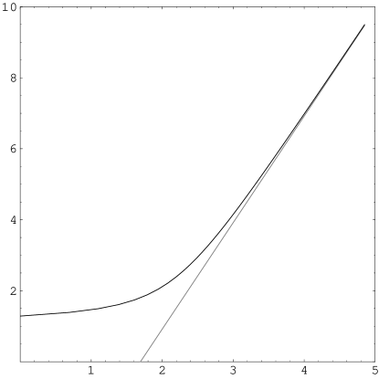
Figure 9: $\mathfrak{L}^{(0)}(d)$ (black curve) in Log-Log coordinates compared to its large-$d$ asymptotics (grey curve, straight line).

Details of the calculation: To compute the integral $\mathfrak{I^{\prime}}$ numerically, it is more convenient to separate the integral over $x\in]0,1]$ and over $x\in[1,\infty[$

$$\mathfrak{I^{\prime}}=\mathfrak{I^{\prime}_{1}}+\mathfrak{I^{\prime}_{2}}\ ,\ \ \mathfrak{I^{\prime}_{1}}=\int_{0}^{1}\mathrm{d}x\,\left[\cdots\right]\ ,\ \ \mathfrak{I^{\prime}_{2}}=\int_{1}^{\infty}\mathrm{d}x\,\left[\cdots\right]\ .$$ (437)

For the second one we can integrate directly the first term, and explicitly the counterterms and get

$$\mathfrak{I^{\prime}_{2}}=-{1\over D}\left[{c_{0}\over d_{0}}\right]^{{2D\over 2-D}}+\mathfrak{I^{\prime\prime}_{2}}\quad,\qquad\mathfrak{I^{\prime\prime}_{2}}=\int_{1}^{\infty}\mathrm{d}x\,x^{D-1}\left[\left[1-{G(x)\over c_{0}}\right]^{-{2D\over 2-D}}\!\!\!-1\right]\ .$$ (438)

For the first one it is better to over-subtract it, in order to improve the integration at $x=0$ and the study of the large-$d$ limit, and write

$$\mathfrak{I^{\prime}_{1}}=-{1\over D}-{D\over(2-D)^{2}(4-D)}\left[{c_{0}\over d_{0}}\right]^{{2D\over 2-D}}+\mathfrak{I^{\prime\prime}_{1}}$$ (439)

$$\mathfrak{I^{\prime\prime}_{1}}=\int_{0}^{1}\mathrm{d}x\,\left[x^{D-1}\left[1-{G(x)\over c_{0}}\right]^{-{2D\over 2-D}}\!\!\!-\left[{c_{0}\over d_{0}}\right]^{{2D\over 2-D}}x^{-D-1}-{1\over 2-D}\left[{c_{0}\over d_{0}}\right]^{{2+D\over 2-D}}x^{-1}+{D\over(2-D)(4-D)}\left[{c_{0}\over d_{0}}\right]^{{2D\over 2-D}}x^{1-D}\right]\ .$$ (440)

Both integrals $\mathfrak{I^{\prime\prime}_{1}}$ and $\mathfrak{I^{\prime\prime}_{2}}$ are convergent for any $D<2$ and have a smooth limit when $D\to 2$.

VII.4 Do the limit $d\to\infty$ and the limit $\epsilon\to 0$ commute?

VII.4.1 An apparent paradox

For $\epsilon>0$ the variational approximation $L^{(0)}$ for $L$ has a regular large-$d$ limit. We have studied it already in Sect. V.4.2. It is of order $\mathcal{O}(d)$ and is given by the convergent integral

$$\mathfrak{L}^{(0)}=d\left(1-{1\over 4-\epsilon}\,\text{f.p.}\int_{0}^{\infty}\mathrm{d}x\,x\,\left[\mathrm{e}^{(4-\epsilon)K_{0}(x)}-1\right]\right)\ ,$$ (441)

which is the large-$d$ limit of the integral (429) ($K_{0}(x)$ is the Modified Bessel function of the 2nd kind).

This integral can be computed numerically. To study its UV structure, we use the small $x$ expansion for the 2D propagator

$$K_{0}(x)\ =\ -\log(x/2)-\gamma_{E}+{1\over 4}x^{2}\left(-\log(x/2)+1-\gamma_{E}\right)+\mathcal{O}(x^{4})$$ (442)

The integrand in (442) behaves at small $x$ as

$$\left[{\mathrm{e}^{\gamma_{E}}/2}\right]^{\epsilon-4}\,\left(x^{\epsilon-3}+{4-\epsilon\over 4}x^{\epsilon-1}\left(-\log(x/2)-\gamma_{E}+1\right)+\mathcal{O}(x^{1+\epsilon}\log x)\right)\,-1\ .$$ (443)

The first term $x^{\epsilon-3}$ gives the UV pole at $\epsilon=2$, and is subtracted by the f.p. prescription. The second term $x^{\epsilon-1}$ gives the poles at $\epsilon=0$ but the $\log x$ gives in fact a double pole, so that

$$\mathfrak{L}^{(0)}\ \simeq\ -\,d\ 4\mathrm{e}^{-4\gamma_{E}}\left({1\over\epsilon^{2}}+{3\over 4\,\epsilon}+\mathcal{O}(1)\right)\ .$$ (444)

There seems to be a discrepancy between this calculation and the results of the previous section:

• Here we take the limit $d\to\infty$, then $\epsilon\to 0$; $\mathfrak{L^{(0)}}$ has a UV pole $\propto{d/\epsilon^{2}}$

• Previously we took the limit $\epsilon\to 0$, then $d\to\infty$; $\mathfrak{L^{(0)}}$ has a UV pole $\propto{d^{2}/\epsilon}$

Clearly the limits $\epsilon\to 0$ and $d\to\infty$ do not simply commute.

VII.4.2 Resolution of the paradox

This apparent paradox can be understood if we use the results of the previous section to study carefully how the bare quantity $\mathfrak{L}^{(0)}=d-\mbox{tr}[{\mathbb{O}}^{(0)}]$ behaves when both $\epsilon\to 0$ and $d\to\infty$. $\mathfrak{L}^{(0)}$ is given by (429) and in that limit the dominant contribution is the integral $\mathfrak{I}$, and more precisely the terms of order $x^{-1}$ when $x\to 0$ in the integral (431) for $\mathfrak{I}$. There are two such terms, the dominant one of order $x^{\epsilon-1}$ (which will give the UV pole at $\epsilon=0$), and the subdominant one of order $x^{\epsilon+1-D}$. These two terms combine so that in the large-$d$, small-$\epsilon$ limit, we have

$$\mathfrak{L}^{(0)}\ \simeq\ -\,{d^{2}\over\epsilon}\,+\,{d^{2}\over\epsilon+2-D}\quad\text{with}\quad\epsilon=2D-{d\over 2}(2-D)\ .$$ (445)

If we take the limit $\epsilon\to 0$ with $d$ finite and large (hence $2-D$ small but non-zero) the first term is singular, and we recover the standard single UV pole, while the second one stays finite. Renormalization within the MS-scheme amounts to subtracting the first term and we recover

$$\mathfrak{L}^{(0)}_{\text{\tiny{MS-D}}}\ \simeq\ {d^{2}\over 2-D}\ =\ {d^{3}\over 4D}\ .$$ (446)

All the other terms contributing to $\mathfrak{L}^{(0)}_{\text{ren}}$ are at most of order $d^{2}$. Thus we recover the fact that the renormalized $\mathfrak{L}$ is of order $\mathcal{O}(d^{3})$.

If we now take the limit $d\to\infty$ with $\epsilon$ non-zero but small, we rewrite (445) as

$$\mathfrak{L}^{(0)}\ \simeq\ -\,{d^{2}(2-D)\over\epsilon(\epsilon+2-D)}\ =\ -{2d(2D-\epsilon)\over\epsilon(\epsilon+2-D)}\ \simeq\ -\,{8d\over\epsilon^{2}}$$ (447)

and we recover the fact that the bare $\mathfrak{L}$ is of order $\mathcal{O}(d)$ but with a double pole when $\epsilon\to 0$. Thus (445) contains both (446) and (447).

VII.4.3 Discussion

Of course in the full theory, it is the first limit ($\epsilon\to 0$ then $d\to\infty$) which must be considered to study the large-$d$ behavior of the renormalized theory. At the level of the variational approximation framework, from the previous calculations one can show that at large-$d$ the variational renormalized $\log\det$ $\mathfrak{L}^{(0)}_{\text{\tiny{MS-D}}}$ has a regular large-$d$ asymptotic expansion in powers of $1/d$,

$$\mathfrak{L}^{(0)}_{\text{\tiny{MS-D}}}\ =\ \mathfrak{l^{0}_{0}}\,d^{3}+\mathfrak{l^{0}_{1}}\,d^{2}\,+\,\mathfrak{l^{0}_{2}}\,d\,+\,\mathfrak{l^{0}_{3}}\,d^{0}\,+\,\cdots$$ (448)

with the $\mathfrak{l^{0}_{n}}$’s real and finite.

Indeed, setting $\epsilon=0$, starting from (434), using equations (437)-(440) and the fact that $c_{0}/d_{0}$ is analytic in $1/d$ ($c_{0}/d_{0}=1+\mathcal{O}(1/d)$), one sees that the only possible non-analytic terms are the integrals $\mathfrak{I^{\prime\prime}_{1}}$ and $\mathfrak{I^{\prime\prime}_{2}}$. Now the mass$=1$ propagator $G(x)$ is analytic in $1/d\sim 2-D$, except at $x=0$, where it has a $\log(x)$ singularity when $D=2$. At $x=\infty$ it behaves as $\exp(-x)$ for any $D$ and it is then easy to see that $\mathfrak{I^{\prime\prime}_{2}}$ is analytic in $1/d$. The integral $\mathfrak{I^{\prime\prime}_{1}}$ given by (440) behaves at $D=2$ as $\int_{0}\mathrm{d}x\,x\,\log x$ and its $n^{\text{th}}$ derivative with respects to $D$ behaves as $\int_{0}\mathrm{d}x\,x\,\log^{n}x$ and is convergent for any $n$. Hence we deduce that $\mathfrak{I^{\prime\prime}_{1}}$ too has an (asymptotic) expansion in $2-D\sim 1/d$. Q.E.D.

Thus the variational renormalized theory at $\epsilon=0$ scales with $d$ as $d^{3}$ (and not as $d$), but still is amenable by a $1/d$ expansion. As we shall see in the next section, the situation becomes more complicated when we deal with the corrections to the variational approximation. Indeed, the perturbative expansion studied in Sect. VI is plagued with infra-red (IR) divergences at $\epsilon=0$, in addition to the UV divergences, and we shall argue that this means that the renormalized theory contains non-analytic terms such as $\log(d)$’s in the large-$d$ limit.

VII.5 Renormalized theory: first $1/d$ correction and IR divergences

VII.5.1 The IR divergences at $\epsilon=0$

In section VI we have isolated the classes of diagrams in the expansion of the kernel ${\mathbb{Q}}$ which give a contribution of order $\mathcal{O}(1)$ in $\mathfrak{L}=\mbox{tr}\log[{1\mathrm{l}}-{\mathbb{Q}}]$. This analysis is valid provided that $\epsilon>0$. Indeed, as long as $\epsilon>0$ the individual diagrams are IR and UV convergent, and the summation over the diagrams in each class in also convergent.

If we now take the limit $\epsilon\to 0$, IR problems may occur when summing these diagrams.

First we consider the diagrams that contribute to $\mbox{tr}[{\mathbb{Q}}^{(1)}]$, depicted in (392). In each of the 11 classes of diagrams in (392) the sum over the $n$ lines joining the left to the right contribute to a similar sum as the sum considered in Sect. V.4.1 at leading order, i.e. to integrals of the form

$$\int_{\mathsf{x}}\int_{\mathsf{k}}\left(\mathrm{e}^{-\mathsf{k}^{2}(c_{0}-G(\mathsf{x}))}-\mathrm{e}^{-\mathsf{k}^{2}(c_{0})}\right)\,\times\cdots\ \simeq\ 2c_{0}\int_{\mathsf{x}}\left(\left[1-G(\mathsf{x})/c_{0}\right]^{-d/2}-1\right)\,\times\cdots$$

These integrals are UV and IR finite when $\epsilon>0$ (with a finite-part prescription to deal with the singularity at $\mathsf{x}=0$). When $\epsilon=0$ they are still IR finite (the $\mathsf{x}$-integration is convergent at $|\mathsf{x}|\to\infty$ since the propagator $G(\mathsf{x})$ is massive, hence exponentially decaying at large distance). On the other hand, these integrals are UV divergent when $\epsilon=0$ (there is a singularity at $\mathsf{x}=0$ which gives a $1/\epsilon$ UV pole) but this divergence is dealt by the renormalization procedure.

Now the second infinite sum in the 11 classes of (392) is given by the “chain-of-bubbles” propagator of the $1/d$ expansion

$$H(\mathsf{p})\,=\,\includegraphics[scale={.5}]{bbline0}\,=1+\parbox{28.5pt}{\includegraphics[scale={.5}]{onebubble}}+\parbox{58.0pt}{\includegraphics[scale={.5}]{twobubble}}+\parbox{87.0pt}{\includegraphics[scale={.5}]{threebubble}}+\cdots$$

given by (352) and depicted in Fig.6. Combining the results of sect. VI.1, in particular (352), (353) and (357), we easily obtain that in the limit $d\to\infty$, $\epsilon$ finite, this propagator is

$$H(\mathsf{p})\ =\ \left[1-\left(1-{\epsilon\over 4}\right)J(p)\right]^{-1}\quad\text{with}\qquad J(p)\,=\,{2\over p}{\mathrm{arcsinh}(p/2)\over\sqrt{1+p^{2}/4}}\,=\,\pi\,B(\mathsf{p})$$ (449)

(we use the notations of DavidWiese1998 for $J(p)$, $B(\mathsf{p})$ is the bubble amplitude (353) at $D=2$). For large $p$ the UV behavior of $H$ is

$$H(p)\,\simeq\ 1+(4-\epsilon){\log p\over p^{2}}+\cdots\quad\text{as}\quad p\to\infty$$ (450)

and does not raise additional UV problems. For small $p$ its IR behavior is

$$H(p)\,\simeq\ {1\over{p^{2}/6}+{\epsilon/4}}\quad\text{as}\quad p\to 0\ .$$ (451)

As long as $\epsilon>0$, the IR behavior of $H$ is that of a massive scalar field with effective mass

$$m_{\text{eff}}=\sqrt{3\epsilon/2}\ \ ,$$ (452)

to be compared with the variational mass $m_{\text{var}}=1$. However, when $\epsilon=0$, this propagator becomes massless $m_{\text{eff}}=0$ and since we are dealing with an effective theory in two dimensions ($D=2$), IR divergences occur! Indeed, in the diagrams of (392) there are two sources of IR divergences:

1. Firstly, the mass shift depicted by is given by the solution of (367) which involves tadpole diagrams with the propagator $H(\mathsf{p})$ at zero momentum $\mathsf{p}=0$, which gives potential powerlike IR divergences $\raisebox{1.29167pt}{\includegraphics[scale={.33}]{graph-13a}}\propto H(0)$ since

   $$H(0)={4\over\epsilon}\ .$$

2. Secondly, both the tadpole diagrams in the r.h.s. of (367) and the other diagrams in (392) contain internal loops with the propagator $H(\mathsf{p})$. Integration over the internal loop momentum gives logarithmic IR divergences since

   $$\int_{\mathsf{p}}H(\mathsf{p})\ =\ {3\over 2\pi}\,\log(1/\epsilon)\,+\,\cdots$$

If we now consider the diagrams which contribute to $\mbox{tr}[{\mathbb{Q}}^{(k)}]$, $k\geq 2$, depicted in (394), they also contain the zero-momentum propagator $H(0)=4/\epsilon$. Their amplitudes at large $d$ are given by (399) and have a powerlike IR divergence in $1/\epsilon^{k}$.

This IR problem was in fact first discovered by the authors in DavidWiese1998 , and its significance for the calculation of the instanton action studied. It was shown in DavidWiese1998 that these IR divergences exist for the instanton profile $V(\mathsf{r})$, but cancel in the first $1/d$ correction to the instanton action $\mathcal{S}_{\mathrm{inst}}$. As we shall see now, some partial cancellations of IR divergences also occur in the contributions of the fluctuations around the instanton, but the first $1/d$ correction $\mathfrak{L}^{(1)}_{\mathrm{ren}}$ to the renormalized fluctuation contribution $\mathfrak{L}_{\mathrm{ren}}$ is still IR divergent at $\epsilon=0$.

VII.5.2 Cancellation of IR divergences in the mass shift $\delta_{1}$

We first look at the mass shift $\delta_{1}$ depicted by and solution of (367). We have already computed $\delta_{1}$ in DavidWiese1998 and $\delta_{1}$ is in fact IR finite when $\epsilon\to 0$. We refer to sect. 6.5 and Appendix B of DavidWiese1998 for the details of the calculation, the final result being given by Eqs. (135), (137) & (138) of DavidWiese1998 , i.e. the integral

$$\begin{split}\delta_{1}\ &=\ {4-\epsilon\over 2-\epsilon}\,2\pi\int_{\mathsf{p}}\left(-\log\left[H(\mathsf{p})\right]-\left(1-{\epsilon\over 4}\right)J(\mathsf{p})\right)\\ &=\ {4-\epsilon\over 2-\epsilon}\int_{0}^{\infty}\mathrm{d}p\,p\,\left(-\log\left[1-\left(1-{\epsilon\over 4}\right)J(p)\right]-\left(1-{\epsilon\over 4}\right)J(p)\right)\\ &=\ {4-\epsilon\over 2-\epsilon}\int_{0}^{\infty}\mathrm{d}v\,\sinh v\,\left(-\log\left[1-\left(1-{\epsilon\over 4}\right){v\over\sinh v}\right]-\left(1-{\epsilon\over 4}\right){v\over\sinh v}\right)\\ &=\ 7.5583\dots\quad\text{for}\quad\epsilon=0\ .\end{split}$$ (453)

This integral is IR and UV convergent even for $\epsilon=0$, since it behaves at small $\mathsf{p}$ as $\int_{\mathsf{p}}1$ and at large $\mathsf{p}$ as $\int_{\mathsf{p}}\mathsf{p}^{-4}\log^{2}(\mathsf{p})$.

To prove the IR finiteness of $\delta_{1}$ it is sufficient to rewrite (367) as

$$\raisebox{0.0pt}{\includegraphics[scale={.33}]{graph-13a}}\ =\raisebox{-10.76385pt}{\includegraphics[scale={.33}]{graph-12a}}+\raisebox{-10.76385pt}{\includegraphics[scale={.33}]{graph-11a}}+\raisebox{-10.76385pt}{\includegraphics[scale={.33}]{graph-10a}}=\raisebox{0.0pt}{\includegraphics[scale={.33}]{piece-1}}\left[\raisebox{0.0pt}{\includegraphics[scale={.33}]{piece-5}}\,+\,\raisebox{0.0pt}{\includegraphics[scale={.33}]{piece-3}}\,+\,\raisebox{0.0pt}{\includegraphics[scale={.33}]{piece-4}}\right]=\raisebox{0.0pt}{\includegraphics[scale={.33}]{piece-1}}\left[\raisebox{0.0pt}{\includegraphics[scale={.33}]{graph-13a}}\ \times\raisebox{0.0pt}{\includegraphics[scale={.33}]{piece-2}}\,+\,\raisebox{0.0pt}{\includegraphics[scale={.33}]{piece-3}}\,+\,\raisebox{0.0pt}{\includegraphics[scale={.33}]{piece-4}}\right]\ .$$ (454)

Since no momentum flows through the first (vertical) $H$ line we have

$$\raisebox{-8.61108pt}{\includegraphics[scale={.33}]{piece-1}}\ =\ {1\over 2c_{0}}\,{4\over\epsilon}\ \text{, \qquad while}\qquad\raisebox{-8.61108pt}{\includegraphics[scale={.33}]{piece-2}}\ =\ {d\over 2}B(0)\,=\,{d\over 2}{1\over 4\pi}$$

is finite, and the last two diagrams contain $\log(\epsilon)$ IR divergences. However, one can easily check that these IR divergences cancel. Indeed the coefficient of the log is obtained by using that as long as $\int_{\mathsf{p}}f(\mathsf{p})$ is not itself IR-divergent,

$$\int_{\mathsf{p}}\raisebox{2.15277pt}{\includegraphics[scale={.33}]{bbline0}}f(\mathsf{p}) = \int_{\mathsf{p}}H(\mathsf{p})\times f(0)+\mbox{infrared convergent terms}$$ (455)

$$= \frac{3}{2\pi}\ln(1/\epsilon)f(0)+\mbox{infrared convergent terms}\ .$$

This means that any $H$ line is to be replaced by $\frac{3}{2\pi}\log(1/\epsilon)$ and treated as if no momentum flows through it. We thus obtain

$$\raisebox{-8.61108pt}{\includegraphics[scale={.33}]{piece-3}}\ =\ {3\over 2\pi}\,\log({1/\epsilon})\,{1\over 2c_{0}}\,\raisebox{-8.61108pt}{\includegraphics[scale={.33}]{piece-6}}\,+\,\mathcal{O}(1)\quad\text{with}\qquad\raisebox{-8.61108pt}{\includegraphics[scale={.33}]{piece-6}}\,=\,{d\over 2}\,{1\over 8\pi}$$

while for the second graph

$$\raisebox{-8.61108pt}{\includegraphics[scale={.33}]{piece-4}}\ =\ -\,{3\over 2\pi}\,\log({1/\epsilon})\,{1\over 2}\,+\,\mathcal{O}(1)\ .$$

The coefficient of the $\log(1/\epsilon)$ IR divergences is therefore zero, since

$$\raisebox{-8.61108pt}{\includegraphics[scale={.33}]{piece-3}}+\raisebox{-8.61108pt}{\includegraphics[scale={.33}]{piece-4}}\ =\ {3\over 2\pi}\,\log({1/\epsilon})\,\left({d\over 4c_{0}}{1\over 8\pi}-{1\over 2}\right)\ \simeq\ -{3\over 16\pi}\,\epsilon\log({1/\epsilon})$$

Thus eq. (454) for $\delta_{1}$ is of the form

$$\delta_{1}\ =\ {1\over\epsilon}\left[\delta_{1}+\mathcal{O}(1)\right]\qquad\Rightarrow\qquad\delta_{1}\,=\,\mathcal{O}(1)\qquad\text{when}\qquad\epsilon=0\ .$$ (456)

VII.5.3 IR divergences in ${\mathbb{Q}}^{(1)}$

We now perform the same analysis for the first $1/d$ correction to the Hessian ${\mathbb{Q}}$, ${\mathbb{Q}}^{(1)}$, calculated in Sect.VI. The Fourier transform of ${\mathbb{Q}}^{(1)}$ is given by the graphs of (379). For reasons that will become clear later, let us separate ${\mathbb{Q}}^{(1)}$ into 4 parts

$$\widehat{{\mathbb{Q}}}^{(1)}\ =\ \widehat{{\mathbb{Q}}}^{(1a)}+\widehat{{\mathbb{Q}}}^{(1b)}+\widehat{{\mathbb{Q}}}^{(1c)}+\widehat{{\mathbb{Q}}}^{(1d)}$$ (457)

$\widehat{{\mathbb{Q}}}^{(1a)}$ is the sum of the graphs which contain the mass shift

$$\widehat{{\mathbb{Q}}}^{(1a)}\ =\ 2\raisebox{-10.76385pt}{\includegraphics[scale={.33}]{graph-O-1e}}+2\,\raisebox{-10.76385pt}{\includegraphics[scale={.33}]{graph-O-1f}}+2\,\raisebox{-10.76385pt}{\includegraphics[scale={.33}]{graph-O-13b}}$$ (458)

$\widehat{{\mathbb{Q}}}^{(1b)}$ is the sum of the graphs which are “really irreducible”

$$\begin{split}\widehat{{\mathbb{Q}}}^{(1b)}\ &=\ \raisebox{-10.76385pt}{\includegraphics[scale={.33}]{graph-O-2e}}+\raisebox{-10.76385pt}{\includegraphics[scale={.33}]{graph-O-2f}}+\raisebox{-10.76385pt}{\includegraphics[scale={.33}]{graph-O-6e}}+\raisebox{-10.76385pt}{\includegraphics[scale={.33}]{graph-O-6f}}\\ &+\raisebox{-10.76385pt}{\includegraphics[scale={.33}]{graph-O-14f}}+\raisebox{-10.76385pt}{\includegraphics[scale={.33}]{graph-O-15}}+\raisebox{-10.76385pt}{\includegraphics[scale={.33}]{graph-O-16f}}+\raisebox{-10.76385pt}{\includegraphics[scale={.33}]{graph-O-17e}}+\raisebox{-10.76385pt}{\includegraphics[scale={.33}]{graph-O-17f}}\end{split}$$ (459)

$\widehat{{\mathbb{Q}}}^{(1c)}$ is the sum of the 4 graphs

$$\begin{split}\widehat{{\mathbb{Q}}}^{(1c)}\ &=\ \raisebox{-2.15277pt}{\includegraphics[scale={.33}]{graph-O-14-A}}+\raisebox{-2.15277pt}{\includegraphics[scale={.33}]{graph-O-16g}}+\raisebox{-2.15277pt}{\includegraphics[scale={.33}]{graph-O-17c}}+\raisebox{-2.15277pt}{\includegraphics[scale={.33}]{graph-O-17a}}\end{split}$$ (460)

and $\widehat{{\mathbb{Q}}}^{(1d)}$ is the single remaining graph.

$$\widehat{{\mathbb{Q}}}^{(1d)}\ =\ \raisebox{-2.15277pt}{\includegraphics[scale={.33}]{graph-O-16h}}\ .$$ (461)

$\widehat{{\mathbb{Q}}}^{(1a)}$ is IR finite since the mass shift is IR finite.

$$\widehat{{\mathbb{Q}}}^{(1a)}\ =\ \mathcal{O}(1)\ .$$ (462)

$\widehat{{\mathbb{Q}}}^{(1b)}$ and $\widehat{{\mathbb{Q}}}^{(1c)}$ have a logarithmic IR divergence in $\log(1/\epsilon)$. By the same argument as above, the coefficient of the IR divergence is obtained by removing the $H$ propagator in the graph, so that

$$\widehat{{\mathbb{Q}}}^{(1b)}\ =\ {1\over 2c_{0}}\,{3\over 2\pi}\,\log(1/\epsilon)\,\widehat{\mathbb{D}}^{(1b)}\,+\,\mathcal{O}(1)$$ (463)

with

$$\begin{split}\widehat{\mathbb{D}}^{(1b)}\ &=\ \raisebox{-10.76385pt}{\includegraphics[scale={.33}]{graph-O-2-e}}+\raisebox{-10.76385pt}{\includegraphics[scale={.33}]{graph-O-2-f}}+\raisebox{-10.76385pt}{\includegraphics[scale={.33}]{graph-O-6-e}}+\raisebox{-10.76385pt}{\includegraphics[scale={.33}]{graph-O-6-f}}\\ &+\raisebox{-10.76385pt}{\includegraphics[scale={.33}]{graph-O-14-e}}+\raisebox{-10.76385pt}{\includegraphics[scale={.33}]{graph-O-15-c}}+\raisebox{-10.76385pt}{\includegraphics[scale={.33}]{graph-O-16-d}}+\raisebox{-10.76385pt}{\includegraphics[scale={.33}]{graph-O-17-e}}+\raisebox{-10.76385pt}{\includegraphics[scale={.33}]{graph-O-17-f}}\end{split}\ .$$ (464)

Similarly for $\widehat{{\mathbb{Q}}}^{(1c)}$ we have

$$\widehat{{\mathbb{Q}}}^{(1c)}\ =\ {1\over 2c_{0}}\,{3\over 2\pi}\,\log(1/\epsilon)\,\widehat{\mathbb{D}}^{(1c)}\,+\,\mathcal{O}(1)$$ (465)

with

$$\begin{split}\widehat{\mathbb{D}}^{(1c)}\ &=\ \raisebox{-2.15277pt}{\includegraphics[scale={.33}]{graph-O-14-f}}+\raisebox{-2.15277pt}{\includegraphics[scale={.33}]{graph-O-16-f}}+\raisebox{-2.15277pt}{\includegraphics[scale={.33}]{graph-O-17-g}}+\raisebox{-2.15277pt}{\includegraphics[scale={.33}]{graph-O-17-h}}\end{split}\ .$$ (466)

Finally $\widehat{{\mathbb{Q}}}^{(1d)}$ has an IR pole in $1/\epsilon$, since the bubble propagator carries zero momentum,

$$\widehat{{\mathbb{Q}}}^{(1d)}\ =\ \mathcal{O}(1/\epsilon)\ .$$ (467)

VII.5.4 Partial IR cancellations in $\mbox{tr}[{\mathbb{Q}}^{(1)}]$

Now come the IR cancellations in $\mbox{tr}[{\mathbb{Q}}^{(1)}]$. We first consider the second term. We notice that the diagrams in (464), which contribute in $\widehat{\mathbb{D}}^{(1b)}$, are obtained by two mass insertions in the diagrams which contribute to $\widehat{{\mathbb{Q}}}^{(0)}$,

$$\widehat{{\mathbb{Q}}}^{(0)}\ =\ \raisebox{-2.15277pt}{\includegraphics[scale={.33}]{graph-O-inter-4}}$$ (468)

and more explicitly, since a mass insertion corresponds to (minus) a derivative with respect to $m^{2}$ (where $m$ is the variational mass in the propagators)

$$\widehat{\mathbb{D}}^{(1b)}_{\mathsf{k}_{1},\mathsf{k}_{2}}\ =\ \left.{{1\over 2}{\partial^{2}\over\partial{(m^{2})}^{2}}\,\left({\int_{\mathsf{x}}\left<\mathrm{e}^{\mathrm{i}\mathsf{k}_{1}\mathsf{r}(\mathsf{o})}\,\mathrm{e}^{\mathrm{i}\mathsf{k}_{2}\mathsf{r}(\mathsf{x})}\right>_{m}^{\mathrm{conn}}-d}\right)}\right|_{m=1}\,=\,\left.{{1\over 2}{\partial^{2}\over\partial{(m^{2})}^{2}}\,\widehat{\mathbb{Q}}^{(0)}_{\mathsf{k}_{1},\mathsf{k}_{2}}}\right|_{m=1}\ .$$ (469)

The effect of the derivative on the propagators from $\mathsf{o}$ to $\mathsf{x}$ is easy to understand. The tadpoles with one or two mass insertions are generated by the derivative acting on the circle (365) at $\mathsf{o}$ or $\mathsf{x}$.

The kernel $\widehat{\mathbb{D}}^{(1b)}$ is clearly non-zero, but it is traceless for $\epsilon=0$. Indeed,

$$\mbox{tr}\left[\widehat{\mathbb{D}}^{(1b)}\right]\ =\ \ \left.{{1\over 2}{\partial^{2}\over\partial{(m^{2})}^{2}}\,\mbox{tr}\left[{\mathbb{Q}}^{(0)}\right]}\right|_{m=1}$$ (470)

and $\mbox{tr}\left[{\mathbb{Q}}^{(0)}\right]$ scales with the mass $m$ like

$$\mbox{tr}\left[{\mathbb{Q}}^{(0)}\right]\ =\ m^{D-\epsilon}\,\left.{\mbox{tr}\left[{\mathbb{Q}}^{(0)}\right]}\right|_{m=1}\ .$$ (471)

Therefore, since in the large-$d$ limit, $D=2$, we have

$$\mbox{tr}\left[{\mathbb{D}}^{(1b)}\right]\ =\ -{\epsilon(2-\epsilon)\over 8}\,\mbox{tr}\left[{\mathbb{Q}}^{(0)}\right]$$ (472)

and formally $\mbox{tr}\bigl{[}{\mathbb{D}}^{(1b)}\bigr{]}=0$ when $\epsilon=0$.

Similarly we can compute the IR coefficient $\widehat{\mathbb{D}}^{(1c)}$ for the 3rd term and its trace. We obtain easily the explicit result

$$\mbox{tr}\bigl{[}{\mathbb{D}}^{(1c)}\bigr{]}\ =\ 4\pi\,c_{0}\,{\epsilon^{2}(1-\epsilon/4)}\ =\ d\,\epsilon^{2}/4\ .$$ (473)

It is also zero when $\epsilon\to 0$.

Details of the calculation:

We have

$$\begin{split}\raisebox{-2.15277pt}{\includegraphics[scale={.33}]{graph-O-16-f}}&={1\over 4}\,\left({1\over 4\pi}\right)^{2}\,(-\mathsf{k}_{1}^{2})(-\mathsf{k}_{2}^{2})(-\mathsf{k}_{1}\mathsf{k}_{2})\,\mathrm{e}^{-(\mathsf{k}_{1}^{2}+\mathsf{k}_{2}^{2})c_{0}/2}\\ \raisebox{-2.15277pt}{\includegraphics[scale={.33}]{graph-O-17-g}}&={1\over 2}\,\left({1\over 4\pi}\right)\,(-\mathsf{k}_{1}^{2})(-\mathsf{k}_{1}\mathsf{k}_{2})\,\mathrm{e}^{-(\mathsf{k}_{1}^{2}+\mathsf{k}_{2}^{2})c_{0}/2}\\ \raisebox{-2.15277pt}{\includegraphics[scale={.33}]{graph-O-17-h}}&={1\over 2}\,\left({1\over 4\pi}\right)\,(-\mathsf{k}_{2}^{2})(-\mathsf{k}_{1}\mathsf{k}_{2})\,\mathrm{e}^{-(\mathsf{k}_{1}^{2}+\mathsf{k}_{2}^{2})c_{0}/2}\\ \raisebox{-2.15277pt}{\includegraphics[scale={.33}]{graph-O-14-f}}&=(-\mathsf{k}_{1}\mathsf{k}_{2})\,\mathrm{e}^{-(\mathsf{k}_{1}^{2}+\mathsf{k}_{2}^{2})c_{0}/2}\end{split}$$

we integrate over $\mathsf{k}_{1}=-\mathsf{k}_{2}$ to obtain the trace and we use the fact that

$${d\over 4c_{0}}=4\pi(1-\epsilon/4)$$

Q.E.D.

The final result is therefore that the IR divergence of $\mbox{tr}[{\mathbb{Q}}^{(1)}]$ comes only from the last single diagram in (461), which gives ${\mathbb{Q}}^{(1d)}$! It is a single IR pole in $1/\epsilon$, since

$$\widehat{{\mathbb{Q}}}^{(1d)}_{\mathsf{k}_{1},\mathsf{k}_{2}}={1\over 4}\left({1\over 4\pi}\right)^{2}{1\over 2c_{0}}{4\over\epsilon}({-\mathsf{k}_{1}^{2}})({-\mathsf{k}_{2}^{2}})\mathrm{e}^{-(\mathsf{k}_{1}^{2}+\mathsf{k}_{2}^{2})c_{0}/2}$$ (474)

hence

$$\mbox{tr}[{\mathbb{Q}}^{(1d)}]\ =\ {4\over\epsilon}\left(1-{\epsilon\over 4}\right)^{2}\ .$$ (475)

VII.5.5 IR divergence and the unstable mode

We now look at the IR singularity in the other terms of the expansion for $\mathfrak{L}$,

$$\mathfrak{L}=\mbox{tr}\log[{1\mathrm{l}}-{\mathbb{Q}}]=-\sum_{k=1}^{\infty}{1\over k}\,\mbox{tr}[{\mathbb{Q}}^{k}]\ .$$

We have shown in section VI.5 that the next terms $\mbox{tr}[{\mathbb{Q}}^{k}]$ are of order $\mathcal{O}(1)$ and can be computed explicitly at that order, since they are given by the contribution of two diagrams only (see (393)) in ${\mathbb{Q}}$, namely the single bubble diagram , which is IR finite, and the diagram , which is nothing but the IR divergent diagram of (461). Thus we see that all the IR divergences of $\mathfrak{L}^{(1)}$, i.e. the term of order $\mathcal{O}(1)$ in the $1/d$ expansion of $\mathfrak{L}$ are contained in the last term of (400), namely in the summation of the $\log$ series

$$\mathfrak{L}^{(1)}\ \simeq\ \log\left(2-{4\over\epsilon}\right)\,+\,\text{IR finite (but UV divergent) term when }\epsilon\to 0\ .$$ (476)

Now we have shown in Sect. VI.6 that this IR singular $\log(2-4/\epsilon)$ is nothing but the contribution of the smallest (and negative) eigenvalue of the Hessian $\mathcal{S}^{\prime\prime}[V]$ associated to the unstable eigenmode (dilation) for the instanton

$$\lambda_{\mathrm{min}}=2-{4\over\epsilon}\,<\,0\ .$$ (477)

The conclusion of our analysis of the IR divergence of $\mathfrak{L}=\log\det^{\prime}[\mathcal{S}^{\prime\prime}]$ is that, at least at order $1/d$, the IR divergence can be attributed entirely to the contribution of the smallest eigenvalue. This is in fact quite natural, since IR divergences must come from the large distance properties of the fluctuations around the instanton configuration.

VII.5.6 A conjecture for the large-$d$ behavior of the unstable mode

This IR divergence in our large-$d$ estimate of the negative eigenvalue $\lambda_{\mathrm{min}}$ for the instanton Hessian does not mean that $\lambda_{\mathrm{min}}$ is IR singular when $\epsilon=0$, but rather that $\lambda_{\mathrm{min}}$ does not behave in the same way when $d\to\infty$, depending on whether $\epsilon>0$ or $\epsilon=0$.

• If $\epsilon>0$, we have seen that $\lambda_{\mathrm{min}}=\mathcal{O}(1)$ when $d\to\infty$.

• If $d$ is finite and we take the limit $\epsilon\to 0$, we have also $\lambda_{\mathrm{min}}=\mathcal{O}(1)$, as can be checked explicitly for the case $d=4,\epsilon=0$, where we recover the classical $\phi^{4}_{4}$ instanton for the O($n=0$) model for SAW.

• Therefore we expect that the IR pole in (477) means simply that when we first take $\epsilon=0$, then $d\to\infty$, $\lambda_{\mathrm{min}}$ is no more of order $\mathcal{O}(1)$, but becomes infinite ($\lambda_{\mathrm{min}}\to\infty$).

In fact we conjecture that for the renormalized theory, $\lambda_{\mathrm{min}}$ scales as $d$

$$\lambda_{\mathrm{min}}(\epsilon=0,d)\,\simeq\,\mathcal{O}(d)\quad\text{when}\quad d\to\infty$$ (478)

by analogy with the behavior of the leading term $\mathfrak{L^{(0)}}$ which is found to behave as

$$\begin{split}{d\over\epsilon}\,\cdot\,{1\over\epsilon}&\quad\text{when}\quad d\to\infty\quad\text{then}\quad\epsilon\to 0\\ {d\over\epsilon}\,\cdot\,{d}&\quad\text{when}\quad\epsilon\to 0\quad\text{then}\quad d\to\infty\end{split}$$ (479)

The first ${d\over\epsilon}$ being an UV pole, and only the last ${1\over\epsilon}\sim d$ being IR. Even if this form of the conjecture is not correct, it is clear that once again for the unstable mode the limits $\epsilon\to 0$ and $d\to\infty$ do not commute.

VIII Conclusion

In this paper we have shown how to compute at one loop the fluctuations around the instanton in the self-avoiding manifold model, and how this is related to the normalization for the large order asymptotics for the SAM model. We have shown that the perturbative counterterms which make the SAM model UV finite in perturbation theory do renormalize (at one loop) the instanton contribution. We have constructed a systematic $1/d$ expansion, and studied the first terms of this expansion and the interplay between the $1/d$ expansion and renormalization.

Although we have obtained many results in this article, and checked at one loop the consistency of the instanton calculus for the SAM model, several points deserve further studies:

• It would be interesting to get a better understanding of how to resum the IR divergences present in the $1/d$ expansion for the renormalized theory at $\epsilon=0$, or to find another approximation scheme which does not suffer from IR divergences.

• We have checked that the instanton factor obtained by our method is for $D=1$ (self-avoiding walk) equal to the factor obtained by field theoretical methods. However, it would be interesting in this case to compare the approximate result that we obtain via the large-$d$ limit with the exact result (as was done for the instanton action in DavidWiese1998 ).

• A practical application of the theoretical results obtained in this paper would be to compare our large-order asymptotics with our explicit calculations at 2-loop order for the scaling exponents for the SAM DavWie96 , WieDav97 . Since the non-perturbative effects become small when $d$ is large, it is expected (and checked numerically) that the 2-loop estimates for the critical exponents are reliable for large $d$. Such a study would help our understanding of the domain of validity of the 2-loop calculations, and perhaps suggest better resummation procedures than those used previously.

• For renormalized local field theories, in addition to instantons, other contributions occur in the large-order asymptotics, denoted renormalons. They are associated both to the short-distance behavior of the theory (UV renormalons) and to its large-distance behavior (IR renormalons). We expect that such effects occur also for the SAM model at $\epsilon=0$, since for $D=1$ it is equivalent to the $\phi^{4}$ theory, but it is not known how to treat these renormalon effects (if they are present) in the framework of the SAM model, which is a multi-local theory.

Appendix A Measure and normalizations for the functional integral

In this appendix we precise the normalization for the functional integration over the fields and the treatment of the zero modes.

A.1 DeWitt metric and measure for the functional integral

We consider the free membrane model. The functional measure $\mathcal{D}[r]$ is normalized as follows. We start from the DeWitt metric $G$ over the manifold configuration space $\mathcal{C}=\{\mathsf{r}(\mathsf{x})\}$

$$G(\delta\mathsf{r},\delta\mathsf{r})\ =\ {\mu_{0}^{2}\over 2\pi}\,\int_{\mathcal{M}}\mathrm{d}^{D}{\mathsf{x}}\,|\delta\mathsf{r}(\mathsf{x})|^{2}\ =\ {\mu_{0}^{2}\over 2\pi}\,\|\delta\mathsf{r}\|^{2}_{\scriptscriptstyle 2}\ .$$ (480)

$\|\dots\|_{\scriptscriptstyle 2}$ is the $L_{2}$ norm over $\mathcal{M}$. This metric depends explicitly on an (arbitrary) normalization mass scale $\mu_{0}$.

The corresponding measure is defined (formally) by $\mathcal{D}[\mathsf{r}]=\prod_{\mathsf{x}}\rm\mathrm{d}^{d}\mathsf{r}(\mathsf{x})\,\sqrt{\det G}$. This corresponds to the normalization

$$\int\mathcal{D}[\mathsf{r}]\,\exp\left(-{\mu_{0}^{2}\over 2}\int_{\mathcal{M}\!\!\!}\mathrm{d}^{D}\mathsf{x}\,\mathsf{r}(x)^{2}\right)\ =\ 1\ \ .$$ (481)

With this normalization, a quadratic form $\mathbf{A}$ with kernel $A^{a}_{\ b}$, i.e. $(\mathbf{A}\mathsf{r}(\mathsf{x}))^{a}=\int\mathrm{d}^{D}\mathbf{\mathsf{y}}A^{a}_{\ b}(\mathsf{x},\mathsf{y})\mathsf{r}^{b}(\mathsf{y})$, yields

$$\int\mathcal{D}[\mathsf{r}]\,\exp\left(-{1\over 2}\int_{\mathcal{M}}\!\!\!\mathrm{d}^{D}\mathsf{x}\int_{\mathcal{M}}\!\!\!\mathrm{d}^{D}\mathsf{y}\,\mathsf{r}(x)\mathbf{A}(\mathsf{x},\mathsf{y})\mathsf{r}(\mathsf{y})\right)\ =\ \det\left[\mathbf{A}/\mu_{0}^{2}\right]^{-1/2}\ \ .$$ (482)

To evaluate the partition function for the free membrane

$$Z_{0}\ =\ \int\mathcal{D}[\mathsf{r}]\,\exp\left(-{1\over 2}\int_{\mathcal{M}}\!\!\mathrm{d}^{D}\mathsf{x}\,\nabla\mathsf{r}(\mathsf{x})^{2}\right)\ ,$$

we must treat separately the zero modes $\mathsf{r}_{0}(x)=\mathsf{r}_{0}$ of the scalar Laplacian $\Delta_{\mathsf{x}}$ over $\mathcal{M}$ and the fluctuations $\widetilde{\mathsf{r}}$ orthogonal to the zero mode, $G(\mathsf{r}_{0},\widetilde{\mathsf{r}})=0$. Let $G^{(0)}$ be the metric for the collective coordinate $\mathsf{r}_{0}$ of the zero mode induced on the “moduli space” of minima of the action $\mathsf{r}(\mathsf{x})=\mathsf{r}_{0}$ by the DeWitt metric

$$G(\delta\mathsf{r}_{0},\delta\mathsf{r}_{0})\ =\ {\mu_{0}^{2}\over 2\pi}\int_{\mathcal{M}}\!\!\mathrm{d}^{D}\mathsf{x}\,|\delta\mathsf{r}_{0}|^{2}\ =:\ G_{ab}^{(0)}\delta\mathsf{r}_{0}^{a}\delta\mathsf{r}_{0}^{b}\quad\Rightarrow\quad G_{ab}^{(0)}\,=\,{\mu_{0}^{2}\over 2\pi}\text{Vol}(\mathcal{M})\delta_{ab}\ .$$ (483)

Hence the measure is

$$\mathrm{d}\mu(\mathsf{r}_{0})\ =\ \mathrm{d}^{d}\mathsf{r}_{0}\,\sqrt{\det\bigl{(}G_{ab}^{(0)}\bigr{)}}\ =\ \mathrm{d}^{d}\mathsf{r}_{0}\,\left[{\mu_{0}^{2}\over 2\pi}\text{Vol}(\mathcal{M})\right]^{d/2}\ .$$ (484)

The integration over the modes $\widetilde{\mathsf{r}}$ orthogonal to the zero modes gives

$$\left({\det}^{\prime}\left[-\Delta/\mu_{0}^{2}\right]\right)^{-d/2}\ ,$$ (485)

where ${\det}^{\prime}$ is the reduced determinant, that is the product over the non-zero eigenvalues of the operator $-\Delta/\mu_{0}^{2}$. Hence

$$Z_{0}\ =\ \int\mathrm{d}\mu[\mathsf{r}_{0}]\,\left({\det}^{\prime}\left[{-\Delta/\mu_{0}^{2}}\right]\right)^{-d/2}\ =\ \int\mathrm{d}^{d}\mathsf{r}_{0}\ \mathcal{Z}_{0}$$ (486)

with the partition function for the marked manifold $\mathcal{Z}_{0}$

$$\mathcal{Z}_{0}\ =\ \left({{\det}^{\prime}\left[{-\Delta\over\mu_{0}^{2}}\right]{2\pi\over\mu_{0}^{2}\,\text{Vol}(\mathcal{M})}}\right)^{-d/2}\ .$$ (487)

A.2 Zeta-function regularization

The ${\det}^{\prime}$ requires UV regularization for its definition. We use the standard zeta-function regularization (see for instance GBU and Dup87 ).

$$\log({\det}^{\prime}[-\Delta/\mu_{0}^{2}])\ =\ {\mbox{tr}}^{\prime}(\log[-\Delta/\mu^{2}_{0}])\ =\ -\,\left.{\mathrm{d}\over\mathrm{d}s}\zeta(s)\right|_{s=0}\ ,$$ (488)

where the zeta-function $\zeta(s)$ for the operator $A=-\Delta/\mu^{2}_{0}$ is defined by the sum over the non-zero eigenvalues $\lambda_{i}$

$$\zeta_{A}(s)\ =\ \sum_{{\begin{smallmatrix}\lambda_{i}\neq 0\end{smallmatrix}}}\lambda_{i}^{-s}$$ (489)

for $\mathrm{Re}(s)$ large enough, and by analytic continuation down to $s=0$. ${\mbox{tr}}^{\prime}$ means the trace over the subspace orthogonal to $\mathrm{Ker}(A)$ ( w.r.t. to the metric $G$).

The operator $-\Delta$ scales with the internal size $L$ of the manifold $\mathcal{M}$ as $L^{-2}$. Therefore $\zeta(s)$ scales as

$$\zeta(s)\ =\ (L\mu_{0})^{2s}\,\bar{\zeta}(s)\ ,$$ (490)

where $\bar{\zeta}(s)$ is a scale invariant zeta function which depends on the shape of $\mathcal{M}$ but not on its size $L$.

If there is no global conformal anomaly, $\zeta(s)$ is analytic around $s=0$ and $\zeta^{\prime}(0)=\bar{\zeta}^{\prime}(0)+2\log(L\mu_{0})\zeta(0)$. Moreover, for any such $A$, one has

$$\zeta_{A}(0)\ =\ -\,\mathrm{dim}(\mathrm{Ker}(A))\ =\ -\,\text{number of zero modes of}\ A\ .$$ (491)

Indeed, one can show that if $A$ has no zero-mode, for instance $A=-\Delta+m^{2}$, then $\zeta_{A}(0)=\mbox{tr}(1)=0$ (this is analogous to the celebrated rule $\delta(0)=0$ in dimensional regularization), and if $A$ has $N$ zero modes, $\zeta_{A}(s)=\lim_{\epsilon\to 0}[\zeta_{A+\epsilon}(s)-N\epsilon^{-s}]$, therefore $\zeta_{A}(0)=\lim_{\epsilon\to 0}[\zeta_{A+\epsilon}(0)-N]=-N$. The Laplacian $\Delta$ has one zero mode, and therefore

$$\zeta(0)\ =\ -1\quad,\quad\zeta^{\prime}(0)\ =\ \bar{\zeta}^{\prime}(0)-2\log(L\mu_{0})\ .$$ (492)

Using the fact that the size of the manifold is defined as

$$L\ =\ \mathrm{Vol}(\mathcal{M})^{1/D}$$ (493)

we obtain for the partition function

$$\mathcal{Z}_{0}\ =\ L^{d(2-D)/2}\left[{\mathrm{e}^{\bar{\zeta}^{\prime}(0)}\over 2\pi}\right]^{d/2}\ .$$ (494)

The dependence on the mass scale $\mu_{0}$ used to define the measure $\mathcal{D}[\mathsf{r}]$ has disappeared, as expected in the absence of a conformal anomaly.

A.3 Conformal anomaly

It is known that there is no conformal anomaly if

1. $D=1$ and the manifold has no boundary (closed loop). This corresponds to a ring polymer.

2. $D=2$, the manifold has no boundary and has Euler characteristics $\chi=0$. This corresponds to a closed membrane with the topology of a torus (or a Klein bottle).

3. $D$ non-integer. The model is defined by dimensional regularization, as detailed in GBU . This is the relevant case for the $\epsilon$-expansion.

If there is a conformal anomaly, $\zeta(0)\neq-1$ and there is an additional power of $L\mu_{0}$ in the partition function $\mathcal{Z}_{0}$, which depends explicitly on the scale $\mu_{0}$. For instance for $D=2$ (membrane) it is known that

$$\zeta(0)\ =\ -1\,+{c\over 6}\chi\quad,\quad\text{with}\ c=1\ \text{the central charge for the free boson}\ .$$ (495)

Hence

$$\mathcal{Z}_{0}\ \propto\ (L\mu_{0})^{\chi\,d/6}\ .$$ (496)

Appendix B Integration paths for the functional integration over $V[r]$

In this appendix we discuss in more detail via the steepest descent method the functional integration over $V(\mathsf{r})$ and the relative position of the instanton $V^{\mathrm{inst}}$ and of the integration contour over $V$, as the argument $\theta$ of the coupling constant $b$ varies in $[-\pi,\pi]$. This is required to treat properly the contribution of the unstable eigenmode of the Hessian $\mathcal{S}^{\prime\prime}[V]$ for the instanton.

For general $\theta\in[-\pi,\pi]$ we know from (76) that the functional integral for the rescaled potential $V(\mathsf{r})$ is normalized so that

$$\int\mathcal{D}[V]\,\exp\left({\mathrm{e}^{-\mathrm{i}\theta}\over 2g}\int\mathrm{d}^{d}\mathsf{r}\,V(\mathsf{r})^{2}\right)\ =\ 1$$ (497)

($g$ is real positive). The effective action for $V$ is given in (83)

$$\mathcal{S}_{\theta}[V]\ =\ \mathcal{E}[V]\,-{\mathrm{e}^{-\mathrm{i}\theta}\over 2}\,\int\mathrm{d}^{d}\mathsf{r}\,V(\mathsf{r})^{2}$$ (498)

and for large $V$ is dominated by the last term $\int V^{2}$. The steepest descent integration path for $V(\mathsf{r})$ in $\mathbb{C}$ is such that (at least for large $|V|$)

$${\mathrm{Arg}}(V)\ =\ {\pi+\theta\over 2}$$ (499)

(see figure). Thus it turns anti-clockwise from the positive real axis for $\theta=-\pi$ to the imaginary axis for $\theta=0$ to the negative real axis for $\theta=\pi$.

Figure 10: Integration path for $V$ as a function of $\theta={\mathrm{Arg}}(b)$

For general $\theta$ the instanton $V^{\mathrm{inst}}_{\theta}$ is an extremum of $\mathcal{S}_{\theta}[V]$. For negative coupling ($\theta=\pm\,\pi$), the instanton is known. It is the solution found and studied in DavidWiese1998 , $V^{\mathrm{inst}}_{\pm\pi}=V^{\mathrm{inst}}$; it is real and negative; it lies on the steepest descent integration path given by Eq. (499). Let us start from the case $\theta=\pi$, i.e. $b$ lies above the discontinuity along the negative real axis, and look at what happens when $\theta\to 0$. From the solution for the instanton at $\theta=\pi$, $V^{\mathrm{inst}}(\mathsf{r})$, the instanton for general $\theta<\pi$ , $V^{\mathrm{inst}}_{\theta}(\mathsf{r})$, is obtained by analytic continuation from real $\mathsf{r}$ to complex $\mathsf{r}$. Indeed, we know from DavidWiese1998 that for a general $V(\mathsf{r})$, under a scale transformation

$$V(\mathsf{r})\ \to\ V_{\lambda}(\mathsf{r})\ =\ \lambda^{{2D\over 2-D}}V(\lambda\mathsf{r})$$ (500)

the two terms in the effective action $\mathcal{S}[V]$ scale respectively as

$$\mathcal{E}[V_{\lambda}]\ =\ \lambda^{{2D\over 2-D}}\,\mathcal{E}[V]\qquad;\qquad\int_{\mathsf{r}}V_{\lambda}^{2}\ =\ \lambda^{{2\epsilon\over 2-D}}\int_{\mathsf{r}}V^{2}\ .$$ (501)

If we assume that the instanton $V^{\mathrm{inst}}(\mathsf{r})$, obtained in DavidWiese1998 for real $\mathsf{r}$, can be continued analytically to complex $\mathsf{r}$’s, then it is enough to take instead of a real scaling factor $\lambda$ a complex phase factor

$$\lambda\ =\ \mathrm{e}^{\mathrm{i}\omega}$$ (502)

and to choose as phase

$$\omega^{+}_{\theta}\ =\ (\pi-\theta){2-D\over 2(D-\epsilon)}$$ (503)

to know that

$$\left(\mathrm{e}^{\mathrm{i}\omega}\right)^{{2D\over 2-D}}\,V^{\mathrm{inst}}\left(\mathrm{e}^{\mathrm{i}\omega}\mathsf{r}\right)$$ (504)

with $\omega=\omega_{\theta}^{+}$ an extremum of $\mathcal{S}_{\theta}[V]$. Therefore the instanton for $\theta<\pi$ is

$$V^{\mathrm{inst}}_{\theta}(\mathsf{r})\ =\ \mathrm{e}^{\mathrm{i}(\pi-\theta){D\over(D-\epsilon)}}\,V^{\mathrm{inst}}\left(\mathrm{e}^{\mathrm{i}(\pi-\theta){2-D\over 2(D-\epsilon)}}\mathsf{r}\right)\ .$$ (505)

It is clear that this instanton $V^{\mathrm{inst}}_{\theta}$ is now a complex field configuration, since it involves both a“global Wick rotation” in $\mathsf{r}$ space and the multiplication by a global phase. In particular for $\theta=0$ (real positive coupling constant) the instanton is

$$V^{\mathrm{inst}}_{\theta=0}(\mathsf{r})\ =\ \mathrm{e}^{\mathrm{i}\pi{D\over(D-\epsilon)}}\,V^{\mathrm{inst}}\left(\mathrm{e}^{\mathrm{i}\pi{2-D\over 2(D-\epsilon)}}\mathsf{r}\right)\ \ .$$ (506)

The same argument applies for $\theta\in\left]-\pi,0\right]$. If we start from the same real instanton at $\theta=-\pi$ and deform it to $\theta=0$ we obtain another instanton, which is the complex conjugate configuration $\overline{V}^{\mathrm{inst}}_{\theta=0}$ of the instanton obtained by starting from $\theta=\pi$.

How is $V^{\mathrm{inst}}_{\theta}$ located with respect to the steepest descent integration path over $V(\mathsf{r})$? Rather than considering the functional integral over $V(\mathsf{r})$ for real $\mathsf{r}$’s, it is more convenient to rotate the space coordinate $\mathsf{r}$ in the complex plane. This is equivalent to deforming the time contour in the complex plane when dealing with time correlation functions in finite temperature QM and FT. Consider as bulk-space coordinates $\hat{\mathsf{r}}$ defined as

$$\hat{\mathsf{r}}\ =\ \mathrm{e}^{\mathrm{i}\omega^{+}_{\theta}}\,{\mathsf{r}}$$ (507)

and make the change of variables in the functional integral for $V$

$$V(\mathsf{r})\ \to\ \widehat{V}(\hat{\mathsf{r}})=V(\mathsf{r})\quad,\qquad\hat{\mathsf{r}}\ \text{real}\ .$$ (508)

The functional measure becomes $\widehat{\mathcal{D}}[\widehat{V}]$, the measure for $\widehat{V}$, and from (497) it is normalized so that

$$\int\widehat{\mathcal{D}}[\widehat{V}]\,\exp\left({\mathrm{e}^{-\mathrm{i}\theta}\over 2g}\,\mathrm{e}^{-\mathrm{i}d\omega^{+}_{\theta}}\int\mathrm{d}^{d}\hat{\mathsf{r}}\,{\widehat{V}(\hat{\mathsf{r}})}^{2}\right)=1\ .$$ (509)

The steepest descent integration path for $\widehat{V}$ is therefore the line with argument $\widehat{\Omega}^{+}_{\theta}$

$${\mathrm{Arg}}(\widehat{V})\ =\ \widehat{\Omega}^{+}_{\theta}\ =\ {\pi+\theta+d\,\omega^{+}_{\theta}\over 2}\ =\ \pi\,+\,{\pi-\theta\over 2}\,{D\over D-\epsilon}$$ (510)

(remember that $\epsilon=2D-d(2-D)/2$). In the new variable $\widehat{V}$ the instanton differs from the original real instanton $V^{\mathrm{inst}}$ by a pure phase (see Eq. (505))

$$\widehat{V}_{\theta}^{\mathrm{inst}}(\hat{r})\ =\ \mathrm{e}^{\mathrm{i}(\pi-\theta){D\over D-\epsilon}}V^{\mathrm{inst}}(\hat{r})\ .$$ (511)

Since $V^{\mathrm{inst}}$ is real and negative, its argument is $\pi$ and therefore $\widehat{V}_{\theta}^{\mathrm{inst}}(\hat{r})$ has a fixed argument (independent of $\hat{r}$) $\widehat{\Omega}^{\mathrm{inst}}_{\theta}$ given by

$${\mathrm{Arg}}\left(\widehat{V}_{\theta}^{\mathrm{inst}}(\hat{r})\right)\ =\ \widehat{\Omega}^{\mathrm{inst}}_{\theta}\ =\ \pi\,+\,{(\pi-\theta)}\,{D\over D-\epsilon}\ .$$ (512)

For $\theta<\pi$, $\widehat{\Omega}^{\mathrm{inst}}_{\theta}$ is larger than $\widehat{\Omega}^{+}_{\theta}$

$$\widehat{\Omega}^{\mathrm{inst}}_{\theta}\ >\ \widehat{\Omega}^{+}_{\theta}\quad\text{ if}\quad\theta\,<\,\pi\quad\text{and}\quad\epsilon\,<\,D\ .$$ (513)

This means that the instanton lies below the integration path for $\widehat{V}$, see figure 11.

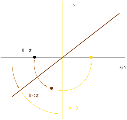
Figure 11: The integration path for $\widehat{V}$ and the instanton $\widehat{V}^{\mathrm{inst}}$ for $\theta=\pi$, $0<\theta<\pi$ and $\theta=0$ (we have set $\epsilon=0$).

When $\theta\to\pi$ the integration path becomes the real axis (with the standard orientation from $-\infty$ to $=\infty$), while the complex instanton $\widehat{V}^{\mathrm{inst}}$ becomes the real (and negative) instanton $V^{\mathrm{inst}}$.

With this result the steepest descent integration prescription for the unstable mode around the instanton at $\theta=\pi$ is fixed. We boldly denote by $V$ this mode. The integration path from $0$ to $-\infty$ has to start from ${V}=0$ (the real vacuum, minimum of the action $\mathcal{S}[V]$), go on the real negative axis up to the instanton $V^{\mathrm{inst}}<0$ which is a local extremum of $\mathcal{S}[V]$ with action $\mathcal{S}^{\mathrm{inst}}=\mathcal{S}[V^{\mathrm{inst}}]>\mathcal{S}[V=0]=0$, then “turn right” (see figure 12) in the upper half complex plane in order for the action to continue to increase, while leaving the instanton below, then go to $-\infty$.

Figure 12: Steepest descent integration paths for the unstable mode for $\theta=\pm\pi$.

The first part of the contour (from $V^{\mathrm{inst}}$ to $\infty$) contributes only to the real part of the partition function $Z$ for negative coupling (and is dominated by the classical vacuum $V=0$). The second part of the contour (from $-\infty$ to $V^{\mathrm{inst}}$) contributes to the imaginary part of $Z$; in fact the dominant contribution to the imaginary part comes from half the Gaussian integral in the imaginary direction at the instanton

$$\int_{V^{\mathrm{inst}}+\mathrm{i}\infty}^{V^{\mathrm{inst}}}\mathrm{d}V$$ (514)

and gives a factor

$$-\,\mathrm{i}\,\,{1\over 2}\left|\det\left(\mathcal{S}^{\prime\prime}[V^{\mathrm{inst}}]\right)\right|^{-1/2}$$ (515)

when compared to the full contribution of the Gaussian integral (the factor $-\mathrm{i}$ comes from the integration path, the factor $1/2$ from the fact that we integrate the unstable mode from $\mathrm{i}\infty$ to $0$, not from $\mathrm{i}\infty$ to $-\mathrm{i}\infty$).

The same argument shows that for $\theta\to-\pi$ the instanton is above the real axis. Therefore for the unstable mode the steepest-descent integration path has to stay below the real axis, with factor

$$\mathrm{i}\,{1\over 2}\,\left|\det\left(\mathcal{S}^{\prime\prime}[V^{\mathrm{inst}}]\right)\right|^{-1/2}\ .$$

These are the results used in Section III.3.2.

Appendix C SAW: $D=1$ SAM versus O($n=0$) field theory

In this appendix we recall the “Laplace-De Gennes” equivalence between the zero-component O($n=0$) $\phi^{4}$ field theory and the (weakly) self-avoiding walk model, which corresponds to the case $D=1$ for the SAM model. The first part of this appendix (sect. 1–3) is basically textbook material, recalled here to fix the notations and the normalizations. We then show that the standard instanton calculus for the O($n=0$) model gives the same result as our instanton calculus for the SAM model in the special case $D=1$. This provides an important check for the consistency of our method.

C.1 Free Field and Brownian walk:

The action for the scalar free field in $d$-dimensional space is (note the factor $1/4$, which is not the most commonly used )

$$S_{0}[\phi]\ =\ \int_{\mathsf{r}}{1\over 4}(\nabla_{\mathsf{r}}\phi)^{2}\ +\ {m^{2}\over 2}(\phi)^{2}\ .$$ (516)

The 2-points correlation function is

$$G_{0}(\mathsf{r}_{1},\mathsf{r}_{2};m^{2})\ =\ \langle\phi(\mathsf{r}_{1})\phi(\mathsf{r}_{2})\rangle_{0}\ =\ \langle\mathsf{r}_{1}|{1\over-\Delta/2+m^{2}}|\mathsf{r}_{2}\rangle\ =\ \int_{0}^{\infty}\mathrm{d}L\ \mathrm{e}^{-Lm^{2}}\,\langle\mathsf{r}_{1}|\mathrm{e}^{L\Delta/2}|\mathsf{r}_{2}\rangle\ ,$$ (517)

and is the Laplace transform with respect to $L$ of the heat kernel $K(\mathsf{r}_{1},\mathsf{r}_{2};L)=\langle\mathsf{r}_{1}|\mathrm{e}^{L\Delta/2}|\mathsf{r}_{2}\rangle$, which admits the random-walk representation

$$K(\mathsf{r}_{1},\mathsf{r}_{2};L)\ =\ \langle\mathsf{r}_{1}|\mathrm{e}^{L\Delta/2}|\mathsf{r}_{2}\rangle\ =\ \int_{\begin{smallmatrix}\ \\ \ \\ {\scriptscriptstyle\mathsf{r}(0)=\mathsf{r}_{1}}\\ {\scriptscriptstyle\mathsf{r}(L)=\mathsf{r}_{2}}\end{smallmatrix}}\!\!\!\!\mathcal{D}[\mathsf{r}]\,\mathrm{e}^{-\int_{L}{1\over 2}(\dot{\mathsf{r}})^{2}\mathrm{d}s}$$ (518)

with $\dot{r}=dr/ds$. To check the normalization, use the semi-classical estimate for the small-$L$ limit of the r.h.s. of (518), $K\simeq\exp{(-|\mathsf{r}|^{2}/2L)}$ and check that $2\partial K/\partial L=\Delta K$. In particular at coinciding points

$$\langle\phi(\mathsf{r}_{1})^{2}\rangle_{0}\ =\ \langle\mathsf{r}_{1}|{1\over-\Delta/2+m^{2}}|\mathsf{r}_{1}\rangle\ =\ \int_{0}^{\infty}\mathrm{d}L\ \mathrm{e}^{-Lm^{2}}\,\langle\mathsf{r}_{1}|\mathrm{e}^{L\Delta/2}|\mathsf{r}_{1}\rangle$$ (519)

and the heat kernel at coinciding points admits the closed random-walk representation:

$$K(\mathsf{r}_{1},\mathsf{r}_{1};L)\ =\ \langle\mathsf{r}_{1}|\mathrm{e}^{L\Delta/2}|\mathsf{r}_{1}\rangle\ =\ \int_{\begin{smallmatrix}\ \\ \ \\ {\scriptscriptstyle\mathsf{r}(0)=\mathsf{r}(L)=\mathsf{r}_{1}}\end{smallmatrix}}\!\!\!\!\!\!\hskip-20.00003pt\mathcal{D}[\mathsf{r}]\,\mathrm{e}^{-\int_{L}{1\over 2}(\dot{\mathsf{r}})^{2}\mathrm{d}s}\ =\ \left.\mathcal{Z}_{0}(\mathsf{r}_{1})\right|_{D=1;L}\ .$$ (520)

It is the partition function for a closed 1-dimensional membrane (i.e. a closed polymer, or a loop) with length $L$, attached to the point $\mathsf{r}_{1}$. Similarly for the one-loop connected diagram

$$\frac{1}{2}\langle\phi(\mathsf{r}_{1})^{2}\phi(\mathsf{r}_{2})^{2}\rangle_{0}^{\mathrm{conn}}\ = \ \frac{1}{2}\left[\langle\phi(\mathsf{r}_{1})^{2}\phi(\mathsf{r}_{2})^{2}\rangle_{0}\,-\,\langle\phi(\mathsf{r}_{1})^{2}\rangle_{0}\langle\phi(\mathsf{r}_{2})^{2}\rangle_{0}\right]\ =\ \left[\langle\mathsf{r}_{1}|{1\over-\Delta/2+m^{2}}|\mathsf{r}_{2}\rangle\right]^{2}$$ (521)

$$= \int_{0}^{\infty}\mathrm{d}L\ \mathrm{e}^{-Lm^{2}}\,\int_{0}^{L}\,\mathrm{d}L_{1}\,\int\mathcal{D}[\mathsf{r}]\,\delta^{d}(\mathsf{r}(0)-\mathsf{r}_{1})\delta^{d}(\mathsf{r}(L_{1})-\mathsf{r}_{2})\,\mathrm{e}^{-\int_{L}{1\over 2}(\dot{\mathsf{r}})^{2}\mathrm{d}s}$$

$$= \int_{0}^{\infty}\mathrm{d}L\ \mathrm{e}^{-Lm^{2}}\,L^{-1}\,\left.\mathcal{R}_{0}^{(2)}(\mathsf{r}_{1},\mathsf{r}_{2})\right|_{D=1,L}\ .$$

This means that the first derivative w.r.t. $m^{2}$ of the l.h.s. of (521) is the Laplace transform of the 2-point correlation function $\mathcal{R}_{0}^{(2)}$ for a free closed loop with length $L$. Similarly connected correlators of a product of $N$ $\phi^{2}$ operators are associated to $N$-point correlation functions for the closed loop.

C.2 SAW and O($n=0$) field theory:

It is well-know that this equivalence extends to the Edwards Model, defined with the normalizations as in (12). The O($n$)-invariant $\phi^{4}$ model is defined by the action

$$S[\vec{\phi}]\ =\ \int\mathrm{d}^{d}\mathsf{r}\,{1\over 4}\left(\nabla_{r}\vec{\phi}\right)^{2}\,+\,{t\over 2}({\vec{\phi}}^{\ 2})\,+\,{b\over 8}({\vec{\phi}}^{\ 2})^{2}$$ (522)

with $\vec{\phi}$ a $n$-component real vector field:

$$\vec{\phi}\ =\ \{\phi^{a};a=1,n\}$$ (523)

$t=m^{2}$ is the squared mass, $b$ is the coupling constant.

The model is equivalent to the Edwards model of polymer with (weak) 2-chain repulsive contact interaction, as defined by the model of (12) for the $D=1$ case. The equivalence holds thanks to the very same Laplace transform between correlation functions as in the free case ($b=0)$. It is valid to all orders in perturbation theory, that is as an asymptotic series expansion for small $b$. The operator $\frac{1}{2}\vec{\phi}^{2}(\mathsf{r})$ is represented by a $\delta$-distribution, or more formally

$$\frac{1}{2}\vec{\phi}^{2}(\mathsf{r})\ \leftrightarrow\ \int\mathrm{d}^{D}\mathsf{x}\,\delta(\mathsf{r}(\mathsf{x})-\mathsf{r})\ .$$ (524)

For instance, for the 1-point correlators we have

$$\lim_{n\to 0}{2\over n}\left<\frac{1}{2}\vec{\phi}(\mathsf{r}_{1})^{2}\right>\ =\ \int_{0}^{\infty}\mathrm{d}L\,\mathrm{e}^{-Lt}\,\mathcal{Z}(\mathsf{r}_{1})\big{|}_{L}$$ (525)

and for the two-points correlators

$$\lim_{n\to 0}{2\over n}\left<\frac{1}{2}\vec{\phi}(\mathsf{r}_{1})^{2}\,\frac{1}{2}\vec{\phi}(\mathsf{r}_{2})^{2}\right>\ =\ \int_{0}^{\infty}\mathrm{d}L\,\mathrm{e}^{-Lt}\,L^{-1}\mathcal{R}^{(2)}(\mathsf{r}_{1},\mathsf{r}_{2})\big{|}_{L}$$ (526)

etc…

C.3 Instanton calculus and large-orders for the O($n$) field theory

We now recall the principle of instanton calculus and large-order estimates for the scalar O($n$) $\phi^{4}$ field theory, following the standard references. This example is useful, since in the limit of $n=0$ it describes polymers, i.e. $D=1$ membranes. The field is a $n$-component real vector field $\vec{\phi}(r)$, $\vec{\phi}=(\phi^{a};a=1,n)$. The action is the O($n$)-invariant $\phi^{4}$ action

$$S[\vec{\phi}]\ =\ \int\mathrm{d}^{d}r\,{1\over 2}\left(\nabla_{r}\vec{\phi}\right)^{2}\,+\,{t\over 2}({\vec{\phi}}^{\ 2})\,+\,{b\over 8}({\vec{\phi}}^{\ 2})^{2}$$ (527)

$t=m^{2}$ is the squared mass, $b$ the coupling constant. We are interested in observables $O[\vec{\phi}]$ which are local monomials in $\phi$ with degree $d_{o}$ in $\phi$, the simplest being the energy operator $E$

$$E[r_{1}]\ =\ (\vec{\phi})^{2}(r_{1})\qquad;\qquad\hbox{degree}(E)=d_{E}=2\ .$$ (528)

The expectation value for the observable $O$ is given by the standard formula

$$\langle O\rangle\ =\ \int\mathcal{D}[\vec{\phi}]\,O[\vec{\phi}]\,\mathrm{e}^{-S[\vec{\phi}]}\Big{/}\int\mathcal{D}[\vec{\phi}]\,\mathrm{e}^{-S[\vec{\phi}]}\ .$$ (529)

We are interested in the large orders of the perturbative series expansion in $b$. As we have seen, we have to use the dispersion relation in the complex-$b$ plane and consider what happens for small $b$ close to the negative real axis, where $b$ is complex and its argument is close to $\pm\pi$. Therefore we rescale the field

$$\phi\ =\ |b|^{-1/2}\varphi\qquad;\qquad\mathrm{with}\qquad\theta\ =\ \mathrm{Arg}(b)\ .$$ (530)

This gives

$$S[\phi]\ =\ {1\over|b|}\,S_{\theta}[\varphi]\qquad;\qquad S_{\theta}[\varphi]\ =\ \int\mathrm{d}^{d}r\,{1\over 2}\left(\nabla_{r}\varphi\right)^{2}\,+\,{t\over 2}({\varphi}^{\ 2})\,+\,{\mathrm{e}^{\mathrm{i}\theta}\over 8}({\varphi}^{\ 2})^{2}$$ (531)

so that

$$\langle O[\phi]\rangle\ =\ |b|^{-{d_{O}\over 2}}\,\langle O[\varphi]\rangle_{\theta,|b|}\ =\ |b|^{-{d_{O}\over 2}}\,{\int\mathcal{D}[\varphi]\,O[\varphi]\,\mathrm{e}^{-S_{\theta}[\varphi]/|b|}\over\int\mathcal{D}[\varphi]\,\mathrm{e}^{-S_{\theta}[\varphi]/|b|}}\ .$$ (532)

For small positive $b$ the functional integral is dominated by the constant classical saddle point

$$\vec{\varphi}_{0}(\mathsf{r})\ =\ \vec{\varphi}_{0}\ =\ 0$$ (533)

constant and absolute minima of $S_{\theta}$ for $\theta=0$. The functional integral is in fact well defined as long as $-\pi<\theta<+\pi$. Now along the cut at $b<0$, that is for $\theta=\pm\pi$, another real extremum of the action $S_{\theta}$ becomes important, the instanton

$$\vec{\varphi}_{i}\ =\ \vec{\varphi}_{i}(r;r_{0},\vec{u}_{0})\ =\ \varphi_{i}(r-r_{0})\vec{u}_{0}\ .$$ (534)

The instanton is characterized by its position $r_{0}$ in space, and its orientation $\vec{u}_{0}$ in the internal $n$-dimensional space ($\vec{u}_{0}$ being a unit vector in $\mathbb{R}^{n}$). $\varphi_{i}(r)$ is the real finite-action solution of the equation

$$-\Delta_{r}\varphi_{i}\,+\,t\,\varphi_{i}\,-\,{1\over 2}\,(\varphi_{i})^{3}\ =\ 0\ ,$$ (535)

which is rotationally invariant around the origin (i.e. depends only on $|r|$) and is non-zero except for $|r|\to\infty$ (or equivalently $\geq 0$, this is enough to define it uniquely).

The contribution of the instanton in the functional integral is at one loop proportional to

$$\mathrm{e}^{-{1\over|b|}S_{\theta}(\varphi_{i})}\,\left[\mathrm{Det^{\prime}}\left[S_{\theta}^{\prime\prime}(\vec{\varphi}_{i})\right]\right]^{-1/2}\ .$$ (536)

The measure for the collective coordinate $\mathsf{r}_{0}$ (the position of the instanton) is easily obtained, since the metric is

$$h_{ab}\ =\ {1\over 2\pi|b|}\,\int\mathrm{d}^{d}\mathsf{r}\,{1\over d}\,(\partial_{a}\vec{\varphi}_{i}\partial_{b}\vec{\varphi}_{i})\ =\ {1\over 2\pi|b|d}\,\|\vec{\nabla}\varphi_{i}\|_{\scriptscriptstyle 2}^{2}\,\delta_{ab}\ .$$ (537)

Hence the measure is

$$\mathrm{d}\mu(\mathsf{r}_{0})\ =\ \mathrm{d}^{d}\mathsf{r}_{0}\,\left[{1\over 2\pi|b|d}\|\vec{\nabla}\varphi_{i}\|_{\scriptscriptstyle 2}^{2}\right]^{d\over 2}\ .$$ (538)

The measure for the internal coordinate $\vec{u}_{0}$ (the orientation) is

$$\mathrm{d}\mu(\vec{u}_{0})\ =\ \mathrm{d}\vec{u}_{0}\,\left[{1\over 2\pi|b|}\int\mathrm{d}^{d}\mathsf{r}\,{\vec{\varphi}_{i}}^{\,2}\right]^{{n-1\over 2}}\ =\ \left[{1\over 2\pi|b|}\|\vec{\varphi}_{i}\|^{2}_{\scriptscriptstyle 2}\right]^{{n-1\over 2}}$$ (539)

with $\mathrm{d}\vec{u}_{0}$ the standard measure on the unit sphere ${\cal S}_{n-1}$ in ${\mathbb{R}}^{n}$. For the O($n$) invariant observables which are of interest to us, the integration over ${\cal S}_{n-1}$ can be performed explicitly, giving the factor $\Omega_{n}$ (the volume of the unit sphere in $\mathbb{R}^{n}$)

$$\Omega_{n}\ =\ \int_{{\cal S}_{n-1}}\hskip-10.00002pt\mathrm{d}\mu(\vec{u}_{0})\ =\ \mathrm{Vol}({\cal S}_{n-1})\ =\ {2\,\pi^{{n\over 2}}\over\Gamma(n/2)}\ .$$ (540)

Note that this volume factor $\Omega_{n}$ vanishes as $n$ when $n\to 0$. However, since O($n$) invariant observables such as $\vec{\varphi}^{2}/n$ behave in the background of the instanton $\vec{\varphi}_{i}$ as $\varphi_{i}^{\,2}/n$ and are therefore of order $1/n$, the factors $n$ and $n^{-1}$ compensate to give a finite $n\to 0$ limit.

Now the Hessian is a $n\times n$ matrix in internal space,

$$S^{\prime\prime}_{\!ab}(\mathsf{r},\mathsf{r}^{\prime})\ =\ {\partial S_{\theta}(\varphi)\over\partial\varphi_{a}(\mathsf{r})\partial\varphi_{b}(\mathsf{r}^{\prime})}\ =\ \delta_{ab}(-\Delta+t)\,-\,\left(\delta_{ab}\,\vec{\varphi}^{2}/2+\varphi^{a}\varphi^{b}\right)\ .$$ (541)

Hence for the instanton background $\vec{\varphi}_{i}=\varphi_{i}\,\vec{u}_{0}$ the Hessian can be written as the product of the longitudinal operator

$$S^{\prime\prime}_{\!l}\ =\ -\Delta+t-{3\over 2}\varphi_{i}^{2}$$ (542)

times $n-1$ transverse operators

$$S^{\prime\prime}_{\!\perp}\ =\ -\Delta+t-{1\over 2}\varphi_{i}^{2}\ .$$ (543)

$S^{\prime\prime}=S^{\prime\prime}_{\!l}\otimes\left(S^{\prime\prime}_{\!\perp}\right)^{n-1}$ . Note that $S^{\prime\prime}_{\!l}$ has $d$ zero modes ${\psi^{\scriptscriptstyle 0}_{l}}_{\mu}=\partial_{\mu}\varphi_{i}$ and that $S^{\prime\prime}_{\!\perp}$ has one zero mode ${\psi^{\scriptscriptstyle 0}_{\perp}}=\varphi_{i}$, so $S^{\prime\prime}$ has $d+n-1$ zero modes. Thus

$${\det}^{\prime}(S^{\prime\prime})\ =\ {\det}^{\prime}(S^{\prime\prime}_{\!l})\,{\det}^{\prime}(S^{\prime\prime}_{\!\perp})^{n-1}$$ (544)

and in the $n=0$ limit

$${\det}^{\prime}(S^{\prime\prime})\big{|}_{n=0}\ =\ {{\det}^{\prime}(S^{\prime\prime}_{\!l})\over{\det}^{\prime}(S^{\prime\prime}_{\!\perp})}\ .$$ (545)

$S^{\prime\prime}_{\!l}$ has one (and only one) eigenvector $\psi^{-}_{l}$ with negative eigenvalue $\lambda_{l}^{-}<-2t$. Therefore $\det S^{\prime\prime}_{\!l}<0$ .

To understand which signe must be chosen for the square-root of the negative determinant $[{\det(S^{\prime\prime})}]^{-1/2}$ ( $+\mathrm{i}$ or $-\mathrm{i}$ ?) we have to consider the steepest-descent integration path for the global $\varphi$ variable. It has to go from ${\mathrm{Arg}}\varphi=\pi\pm\theta/4$ to $\mp\theta/4$, hence for $\theta=+\pi$ it is as depicted on Fig. 13.

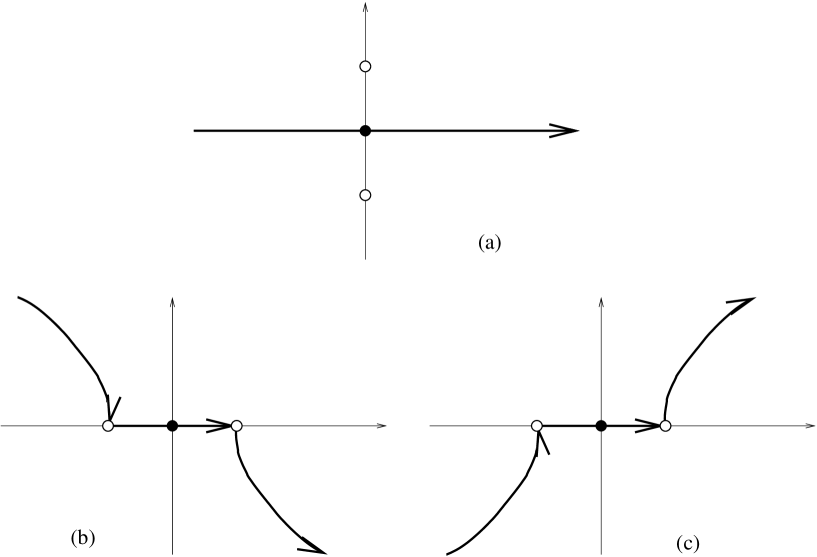
Figure 13: Steepest descent integration path for the global $\varphi$ variable for $\theta=0$ (a), $\theta=\pi$ (b) and $\theta=-\pi$ (c). The black dot represents the classical vacua $\varphi=0$ and the white dots the 2 instanton saddle-points $\varphi=\pm\varphi_{i}$.

Hence the instanton contributes to the imaginary part of an observable by a coefficient

$$\mp{\mathrm{i}\over 2}\left|{\det}^{\prime}(S^{\prime\prime}_{\!l})\right|^{-1/2}\qquad{\mathrm{if}}\qquad\theta=\pm\pi\ .$$ (546)

The rest goes into the real part together with the contribution of the classical vacuum $\varphi_{0}$.

Putting things together, and using Eq. (60) we obtain for the imaginary part at $b<0$ of the e.v. of the O($n$) invariant observable $\cal O$ and for $\mathrm{arg}(b)=\theta=\pm\pi$

$$\mathrm{Im}\langle{O}\rangle \ =\ \mp\,{1\over 2}\,|b|^{-d_{\scriptscriptstyle{O}}/2}\,\mathrm{e}^{-{{1\over|b|}\big{(}S[\varphi_{i}]-S[\varphi_{0}]\big{)}}}\,\left|{{\det}^{\prime}(S^{\prime\prime}_{\!l}[\varphi_{i}])\,\big{(}{\det}^{\prime}(S^{\prime\prime}_{\!\perp}[\varphi_{i})]\big{)}^{n-1}\over\det(S^{\prime\prime}[\varphi_{0}])^{n}}\right|^{-{1\over 2}}\ \times$$

$$\hskip 20.00003pt\,\left[{1\over 2\pi|b|d}\|\vec{\nabla}\varphi_{i}\|_{\scriptscriptstyle{2}}^{2}\right]^{d\over 2}\,\left[{1\over 2\pi|b|}\|\varphi_{i}\|_{\scriptscriptstyle{2}}^{2}\right]^{{n-1\over 2}}\,\Omega_{n}\,\int\mathrm{d}^{d}\mathsf{r}_{\scriptscriptstyle{0}}\,\left(O[\varphi_{i}[\mathsf{r}_{0}]]-O[\varphi_{0}]\right)$$

while of course

$$\mathrm{Re}(\langle{O}\rangle\big{)}\ =\ O(\varphi_{0})\ .$$ (548)

In particular for $n=0$ and $O$ a product of energy operators $E$ defined as

$$O_{1}[\mathsf{r}_{1}]\ = \ \lim_{n\to 0}\,{1\over n}\,\big{(}\vec{\phi}(\mathsf{r}_{1})\big{)}^{2}$$ (549)

$$O_{2}[\mathsf{r}_{1},\mathsf{r}_{2}]\ = \ \lim_{n\to 0}\,{1\over n}\,\big{(}\vec{\phi}(\mathsf{r}_{1})\big{)}^{2}\big{(}\vec{\phi}(\mathsf{r}_{2})\big{)}^{2}$$ (550)

and omitting the $i$ subscript for “instanton”, we obtain

$$\mathrm{Im}\langle O_{1}\rangle = \mp\,\frac{1}{2}\,\ |b|^{-{d+1\over 2}}\,\mathrm{e}^{-{1\over|b|}S_{i}}\,\left|{{\det}^{\prime}S^{\prime\prime}_{\!l}\over{\det}^{\prime}S^{\prime\prime}_{\!\perp}}\right|^{-{\frac{1}{2}}}\,(2\pi)^{{1-d\over 2}}\,\left[{\|\nabla\varphi_{i}\|_{\scriptscriptstyle{2}}^{2}\over d}\right]^{{d\over 2}}\,\|\varphi_{i}\|_{\scriptscriptstyle{2}}$$ (551)

$$\mathrm{Im}\langle O_{1}[\mathsf{r}_{1},\mathsf{r}_{2}]\rangle = \mp\,\frac{1}{2}\,\ |b|^{-{d+3\over 2}}\,\mathrm{e}^{-{1\over|b|}S}\,\left|{{\det}^{\prime}S^{\prime\prime}_{\!l}\over{\det}^{\prime}S^{\prime\prime}_{\!\perp}}\right|^{-{\frac{1}{2}}}\!(2\pi)^{{1-d\over 2}}\,\left[{\|\nabla\varphi\|_{\scriptscriptstyle{2}}^{2}\over d}\right]^{{d\over 2}}\!\!\|\varphi\|_{\scriptscriptstyle{2}}^{-1}\,\varphi^{2}\!\star\varphi^{2}(\mathsf{r}_{1}-\mathsf{r}_{2})$$

$\star$ denotes the usual convolution product $f\star g(\mathsf{r})=\int\mathrm{d}\mathsf{r}^{\prime}f(\mathsf{r}^{\prime})g(\mathsf{r}^{\prime}+\mathsf{r})$. Note also a few useful results

$$\varphi_{0}\ =\ 0\ \rightarrow\ S[\varphi_{0}]\ =\ 0$$ (553)

$$S[\varphi_{i}]\ =\ {1\over 8}\,\int\mathrm{d}^{d}\mathsf{r}\,\varphi_{i}^{4}$$ (554)

$$\int\mathrm{d}^{d}\mathsf{r}\,\big{(}\nabla\varphi_{i}\big{)}^{2}\ =\ -\,t\int\mathrm{d}^{d}\mathsf{r}\,\varphi_{i}^{2}\,+\,{1\over 2}\int\mathrm{d}^{d}\mathsf{r}\,\varphi_{i}^{4}\ .$$ (555)

C.4 Instanton calculus for the SAW model of polymers

Since the Edwards model for SAW is the inverse Laplace transform w.r.t. $t=m^{2}$ of the O($n$) model, instanton calculus must take into account this transformation and is (slightly) modified, as is explained here.

The action for the SAW model is

$$S[\phi]=\int{1\over 4}(\nabla\phi)^{2}+{t\over 2}\phi^{2}-{|b|\over 8}(\phi^{2})^{2}\ .$$ (556)

We have by inverse Laplace transform, for a closed polymer of length $L$

$$\mathcal{Z}(\mathsf{r};L)\ = \ \int_{-\mathrm{i}\infty}^{+\mathrm{i}\infty}{\mathrm{d}t\over 2\mathrm{i}\pi}\,\mathrm{e}^{Lt}\,\langle O_{1}(\mathsf{r};t)\rangle$$ (557)

$$\mathcal{R}(\mathsf{r}_{1},\mathsf{r}_{2};L)\ = \ L\int_{-\mathrm{i}\infty}^{+\mathrm{i}\infty}{\mathrm{d}t\over 2\mathrm{i}\pi}\,\mathrm{e}^{Lt}\,\langle O_{2}(\mathsf{r}_{1},\mathsf{r}_{2};t)\rangle\ .$$ (558)

So we consider the effective action

$$\mathcal{S}[\phi,t]=\int\left[{1\over 4}(\nabla\phi)^{2}+{t\over 2}\phi^{2}-{|b|\over 8}(\phi^{2})^{2}\right]\ -\ t\,L\ .$$ (559)

To factorize $|b|$ and $L$ we must rescale both $\phi$, $t$ and $\mathsf{r}$ with

$$\phi(\mathsf{r})=|b|^{{-d\over 2(d-2)}}\,L^{{-1\over d-2}}\,\sqrt{2}\,\varphi(\mathsf{r}^{\prime})\qquad,\qquad\mathsf{r}=|b|^{{1\over d-2}}\,L^{{1\over d-2}}\,\mathsf{r}^{\prime}\qquad,\qquad t=|b|^{{-2\over d-2}}\,L^{{-2\over d-2}}\tau$$ (560)

The action becomes

$$\mathcal{S}[\phi,t]\ =\ 2\left[|b|L^{\epsilon}\right]^{-{2\over d-2}}{\cal S}[\varphi,\tau]\qquad;\qquad\epsilon={4-d\over 2}\ ,$$ (561)

and the effective action is now

$${\cal S}[\varphi,\tau]\ =\ S[\varphi]-{\tau\over 2}\qquad;\qquad S[\varphi]\ =\ \int\left({1\over 4}(\nabla\vec{\varphi})^{2}+{\tau\over 2}\vec{\varphi}^{2}-{1\over 4}\big{(}\vec{\varphi}^{2}\big{)}^{2}\right)\ .$$ (562)

The effective coupling constant is

$$b_{\mathrm{eff}}={1\over 2}\,\Big{[}|b|L^{\epsilon}\Big{]}^{{2\over d-2}}$$ (563)

instead of $|b|$.

The instanton is given by the saddle point equations

$$\vec{\varphi}\,=\,\varphi\,\vec{u}_{0}\qquad;\qquad-{\Delta\over 2}\varphi+\tau\varphi-\varphi^{3}=0\qquad;\qquad\int\varphi^{2}=1$$ (564)

and the Hessian is

$${\cal S}^{\prime\prime}\ =\ \left[\begin{array}[]{cc }S^{\prime\prime}&\vec{\varphi}\\ \vec{\varphi}^{t}&0\end{array}\right]\ .$$ (565)

It can still be separated into its transverse part, which is $n-1$ times the transverse operator $S^{\prime\prime}_{\!\perp}$

$$S^{\prime\prime}_{\!\perp}=-{\Delta\over 2}+\tau-\varphi^{2}$$ (566)

times the longitudinal part

$${\cal S}^{\prime\prime}_{\!l}\ =\ \left[\begin{array}[]{cc }S^{\prime\prime}_{\!l}&\varphi\\ \varphi^{t}&0\end{array}\right]\qquad;\qquad S^{\prime\prime}_{\!l}=-{\Delta\over 2}+\tau-3\varphi^{2}\ ,$$ (567)

which has $d$ translational zero modes, namely the $\Psi_{\mu}=\left[\begin{array}[]{ c}\psi_{\mu}\\ 0\end{array}\right]$ since $\varphi\cdot\psi_{\mu}=\int\varphi\partial_{\mu}\varphi=\frac{1}{2}\int\partial_{\mu}\varphi^{2}=0$. It is then easy to show, denoting by $P_{0}$ the projector onto the kernel of $S^{\prime\prime}_{\!l}$ generated by its zero modes, and defining the “inverse” of $S^{\prime\prime}_{\!l}$ as

$$\left[{1\over S^{\prime\prime}_{\!l}}\right]^{\prime}\ =\ \big{(}S^{\prime\prime}_{\!l}+P_{0}\big{)}^{-1}\,-\,P_{0}$$ (568)

that

$${\det}^{\prime}{\cal S}^{\prime\prime}_{\!l} = \det\begin{pmatrix}S^{\prime\prime}_{l}+P_{0}&\varphi\\ \varphi^{t}&0\end{pmatrix}\ =\ \det\big{(}S^{\prime\prime}_{l}+P_{0}\big{)}\ \det\big{(}-\varphi^{t}(S^{\prime\prime}_{l}+P_{0})^{-1}\varphi\big{)}$$ (569)

$$= -\,{\det}^{\prime}{S}^{\prime\prime}_{\!l}\,\left(\varphi\cdot\left[{1\over S^{\prime\prime}_{\!l}}\right]^{\prime}\cdot\varphi\right)\ .$$

But it turns out that

$$\left[{1\over S^{\prime\prime}_{\!l}}\right]^{\prime}\cdot\varphi\ =\ -\,{1\over 2\tau}\,(\mathsf{r}\cdot\nabla+1)\varphi\ .$$ (570)

Indeed, one can check that $\mathsf{r}\nabla\varphi$ as well as $\varphi$ are orthogonal to $\psi_{\mu}$ and an explicit calculation shows that

$$\left[-{\Delta\over 2}+\tau-3\varphi^{2}\right](\mathsf{r}\cdot\nabla+1)\varphi\ =\ -2\tau\,\varphi\ .$$ (571)

It follows that the additional factor in the determinant (which comes from the integration over $\tau$ at the saddle point) is

$$-\,\left(\varphi\cdot\left[{1\over S^{\prime\prime}_{\!l}}\right]^{\prime}\cdot\varphi\right)\ =\ {1\over 2\tau}\,\int\varphi(\mathsf{r}\nabla+1)\varphi\ =\ -\,{d-2\over 4\tau}\,\int\varphi^{2}\ =\ -\,{d-2\over 4\tau}$$ (572)

$\tau$ is $>0$ if $d<4$, so this factor is negative for $2<d<4$, but the integration path over $\tau$ is also imaginary (it goes from $-\mathrm{i}\infty$ to $+\mathrm{i}\infty$). Thus the integration over $\tau$ gives the factor

$$(2\pi)^{-1}\,|b|^{{-2\over d-2}}\,L^{{-2\over d-2}}$$ (573)

(coming from the measure ${\mathrm{d}\tau\over 2\mathrm{i}\pi}$) times

$$\left|{2\pi\over{b_{\mathrm{eff}}{d-2\over 4\tau}}}\right|^{1/2}$$ (574)

coming from the Gaussian integration. This gives

$$\left[\pi{d-2\over\tau}\right]^{-1/2}|b|^{{-1\over d-2}}L^{{-d\over 2(d-2)}}\ .$$ (575)

For the observable $\phi^{2}/n$ the integration over the zero modes gives

$$2|b|^{{-d\over d-2}}L^{{-2\over d-2}}\,{\Omega_{n}\over n}\,\int\varphi^{2}\ =\ 2|b|^{{-d\over d-2}}L^{{-2\over d-2}}$$ (576)

times the measure and determinant factors

$$\left[{\|\varphi\|^{2}\over 2\pi b_{\mathrm{eff}}}\right]^{-1/2}\,\left[{\|\nabla\varphi\|^{2}\over 2\pi b_{\mathrm{eff}}d}\right]^{d/2}\,\left|{{\det}^{\prime}S^{\prime\prime}_{l}\over{\det}^{\prime}S^{\prime\prime}_{\perp}}\right|^{-1/2}\ =\ \left[\pi|b|^{{2\over d-2}}L^{{4-d\over d-2}}\right]^{{1-d\over 2}}\,\left[{\|\nabla\varphi\|^{2}\over d}\right]^{d/2}\,\left|{{\det}^{\prime}S^{\prime\prime}_{l}\over{\det}^{\prime}S^{\prime\prime}_{\perp}}\right|^{-1/2}\ .$$ (577)

Putting things together we get

$$\mathrm{Im}\mathcal{Z}(\mathsf{r};L)\ =\ \mp\,{1\over 2}\,L^{{-d\over 2}}\,\big{[}|b|L^{\epsilon}\big{]}^{{-2d\over d-2}}\mathrm{e}^{-{(2S-\tau)\big{[}|b|L^{\epsilon}\big{]}^{{-2\over d-2}}}}\,\left|{\det}^{\prime}S^{\prime\prime}_{\!l}\over{\det}^{\prime}S^{\prime\prime}_{\!\perp}\right|^{-\frac{1}{2}}\,\left[{\|\nabla\varphi\|_{\scriptscriptstyle{2}}^{2}\over\pi d}\right]^{{d\over 2}}\left({d-2\over 4\tau}\right)^{-\frac{1}{2}}\ .$$ (578)

Remember that $|b|L^{\epsilon}$ is dimensionless. We show below that with our normalizations and the equation for the instanton.

$$\tau=(4-d)S\qquad;\qquad\|\vec{\nabla}\varphi\|^{2}=2dS\ .$$ (579)

This simplifies slightly (578)

$$\mathrm{Im}\mathcal{Z}(\mathsf{r};L)\ =\ \mp\,{1\over 2}\,L^{{-d\over 2}}\,\big{[}|b|L^{\epsilon}\big{]}^{{-2d\over d-2}}\mathrm{e}^{-{(d-2)S\,\big{[}|b|L^{\epsilon}\big{]}^{{-2\over d-2}}}}\,\left|{\det}^{\prime}S^{\prime\prime}_{\!l}\over{\det}^{\prime}S^{\prime\prime}_{\!\perp}\right|^{-\frac{1}{2}}\,\left[{2S\over\pi}\right]^{{d\over 2}}\left[{4(4-d)S\over d-2}\right]^{\frac{1}{2}}\ .$$ (580)

C.5 $d\to 4$ limit and scale invariance

The O($n$) model at $d=4$ ($\epsilon=0$) becomes scale invariant and the instanton has an additional zero mode associated with dilations. For the SAW model nothing special occurs when $\epsilon\to 0$ (as far as global scale transformations are concerned). Here we show in detail how the dilation zero mode is absorbed in the transformation O($n$) $\to$ SAW, and the form of the instanton and of the large-order results at $\epsilon=0$.

We first derive a few exact results. If $\varphi$ is the instanton, solution of $(-{\Delta\over 2}+\tau)\varphi-\varphi^{3}=0$ and the Hessian is $S^{\prime\prime}_{\!l}=-{\Delta\over 2}+\tau-{3}\varphi^{2}$ then

$$\left[{1\over S^{\prime\prime}_{\!l}}\right]^{\prime}\varphi = -{1\over 2\tau}(\mathsf{r}\nabla+1)\varphi$$ (581)

$$\left[{1\over S^{\prime\prime}_{\!l}}\right]^{\prime}\varphi^{3} = -\frac{1}{2}\varphi$$ (582)

$$\left(\varphi^{3}\right|\left.(\mathsf{r}\nabla+1)\varphi\right) = \int\varphi^{3}(\mathsf{r}\nabla+1)\varphi=\int\left(1+{\scriptstyle{1\over 4}}\mathsf{r}\nabla\right)\varphi^{4}={\displaystyle{4-d\over 4}}\int\varphi^{4}$$ (583)

$$= -2\tau\left(\varphi^{3}\right.\left[{1\over S^{\prime\prime}_{\!l}}\right]^{\prime}\left.\varphi\right)=-2\tau\left(\varphi\right.\left[{1\over S^{\prime\prime}_{\!l}}\right]^{\prime}\left.\varphi^{3}\right)$$ (584)

$$= \tau\left(\varphi|\varphi\right)=\tau\int\varphi^{2}\ .\ .$$ (585)

The instanton action is

$$S=\int{1\over 4}(\nabla\varphi)^{2}+{\tau\over 2}\varphi^{2}-{{1\over 4}}\varphi^{4}=\int\frac{1}{2}\varphi(-{\Delta\over 2}+\tau)\varphi-{{1\over 4}}\varphi^{4}={{1\over 4}}\int\varphi^{4}\ .$$ (586)

Hence

$$\int\varphi^{2}={4-d\over\tau}S\qquad;\qquad\int(\nabla\varphi)^{2}=2\,d\,S\qquad;\qquad\int\varphi^{4}=4S\ .$$ (587)

Now remember that $\tau$ is fixed by the normalization $\int\varphi^{2}=1$. In the limit $d\to 4$, we must take the limit $\tau\to 0$ to get the finite-action instanton. The general solution of the equation $-\Delta\varphi=2\varphi^{3}$ at $d=4$ is

$$\varphi(\mathsf{r})_{d=4}={2\mathsf{r}_{0}\over\mathsf{r}^{2}+\mathsf{r}_{0}^{2}}\qquad;\qquad\hbox{with corresponding action}\qquad S_{d=4}={2\over 3}\pi^{2}\ .$$ (588)

$\mathsf{r}_{0}$ is the instanton size. The size is arbitrary for the massless $d=4$ theory by scale invariance. For $\mathsf{r}\gg\mathsf{r}_{0}$, $\varphi$ satisfies the linearized equation $-\varphi^{\prime\prime}-{\scriptstyle{d-1\over\mathsf{r}}}\varphi^{\prime}+2\tau\varphi=0$ and is a Bessel function

$$\varphi(\mathsf{r})\propto\mathsf{r}^{1-{d/2}}\mathrm{K}_{d/2-1}(\sqrt{2\tau}\mathsf{r})$$ (589)

and is such that

$$\varphi(\mathsf{r})\simeq C\,\mathsf{r}^{2-d}\qquad{\mathrm{for}}\quad\mathsf{r}_{0}\ll\mathsf{r}\ll 1/\sqrt{\tau}\qquad;\qquad\varphi(\mathsf{r})\propto\mathrm{e}^{-\mathsf{r}\sqrt{2\tau}}\qquad{\mathrm{for}}\quad\mathsf{r}\gg 1/\sqrt{\tau}\ .$$ (590)

To match this behavior with the large-$\mathsf{r}$ behavior of the instanton at $d=4$, the constant $C$ must behave as

$$C(d)=2\mathsf{r}_{0}\,(1+{\cal O}(\varepsilon))\qquad\hbox{with}\qquad\varepsilon=4-d\ .$$ (591)

For fixed $\mathsf{r}_{0}$, we must let $\tau\to 0$, but at which rate? The evaluate this, use the equation (587) which tells us that $\tau\int\varphi^{2}\simeq\varepsilon S_{d=4}$ when $\varepsilon\to 0$. When evaluating $\int\varphi^{2}$ in this limit, it is easy to see that it is the contribution of the domain $\mathsf{r}_{0}\ll\mathsf{r}\ll 1/\sqrt{\tau}$ which dominates the integral, so that

$$\int\varphi^{2} = \Omega_{d}\int_{0}^{\infty}\mathrm{d}\mathsf{r}\,\mathsf{r}^{d-1}\varphi(\mathsf{r})^{2}\simeq 2\,\pi^{2}\int_{\mathsf{r}_{0}}^{1/\sqrt{\tau}}\mathrm{d}\mathsf{r}\,\mathsf{r}^{d-1}\,\left(C\,\mathsf{r}^{2-d}\right)^{2}\simeq 2\,\pi^{2}\,(2\mathsf{r}_{0})^{2}\,\ln(1/\mathsf{r}_{0}\sqrt{\tau})\ .$$

Therefore $\tau$ goes indeed to zero as $d\to 4$ according to

$$\varepsilon=4-d\simeq 6\,\tau\mathsf{r}_{0}^{2}\,\ln\left(1/\tau\mathsf{r}_{0}^{2}\right)\ .$$ (593)

Now if we consider the polymer, we have to keep its length $L=1$ fixed, hence $\int\varphi^{2}=1$. Then the instanton size $\mathsf{r}_{0}$ has to vanish together with $\tau$ as $\varepsilon\to 0$.

$$1={\varepsilon\over\tau}{S}\ \implies\ \tau\simeq{\varepsilon}{2\,\pi^{2}\over 3}\ \implies\ \mathsf{r}_{0}\simeq{1\over 2\pi\sqrt{\ln(1/\varepsilon)}}\ .$$ (594)

Finally, we are interested in the smallest positive eigenvalue $\lambda^{+}$ of the Hessian $S^{\prime\prime}_{\!l}$ and the corresponding eigenvector $\psi^{+}$. As $\varepsilon\to 0$ we expect that $\lambda^{+}\to 0$ and $\psi^{+}\to(\mathsf{r}\nabla+1)\varphi$ the zero-mode for scale transformations. In this limit $\lambda^{+}$ can be estimated as follows

$$(\varphi|\left[{1\over S^{\prime\prime}_{\!l}}\right]^{\prime}\varphi) \simeq (\varphi|\psi^{+}){1\over\lambda^{+}}(\psi^{+}|\varphi){1\over(\psi^{+}|\psi^{+})}\ .$$ (595)

But the l.h.s. is equal to

$$-{2-d\over 4\tau}(\varphi|\varphi)\simeq{1\over 2\,\tau}(\varphi|\varphi)\ =\ {1\over 2\,\tau}\ .$$ (596)

Using the asymptotics obtained for $\varphi$ in the $\varepsilon\to 0$ limit

$$\varphi(\mathsf{r})\simeq 2\,\mathsf{r}_{0}\,\mathsf{r}^{-2}\ \implies\ \psi^{+}(\mathsf{r})\simeq-2\,\mathsf{r}_{0}\,\mathsf{r}^{-2} \qquad\hbox{for}\quad\mathsf{r}_{0}\ll\mathsf{r}\ll 1/\sqrt{\tau}$$ (597)

we obtain

$$(\psi^{+}|\varphi)\simeq-(\varphi|\varphi)=-1\qquad(\psi^{+}|\psi^{+})\simeq(\varphi|\varphi)=1 \qquad\hbox{for}\quad\varepsilon\to 0\ .$$ (598)

Hence the smallest positive eigenvalue of $\mathcal{S}^{\prime\prime}_{\!l}$ vanishes as $\varepsilon$ when $d\to 4$, as expected

$$\lambda^{+}\simeq 2\,\tau\,\simeq\,{4\pi^{2}\over 3}\,\varepsilon\qquad\hbox{for}\quad\varepsilon\to 0\ .$$ (599)

Thus in the limit $d\to 4$ the Hessian $S^{\prime\prime}_{\!l}$ gets an additional zero mode, so that the zero-mode subtracted determinant $\det^{\prime}$ is discontinuous at $d=4$ ($\lim_{d\to 4}{\det}^{\prime}\left[S^{\prime\prime}_{\!l}\right]\neq{\det}^{\prime}\left[\lim_{d\to 4}S^{\prime\prime}_{\!l}\right]$), but we can write in the semiclassical estimates

$${\det}^{\prime}\left[S^{\prime\prime}_{\!l}\right]\quad\simeq_{d\to 4}\quad\lambda^{+}\cdot{\det}^{\prime}\left[S^{\prime\prime}_{\!l}\big{|}_{d=4}\right]\ .$$ (600)

The singular factor $\tau^{\frac{1}{2}}$ in eq. (578), which comes from the integration over $t$, is canceled by the $\lambda^{+}$ in ${\det}^{\prime}S^{\prime\prime}_{\!l}$, as expected, since we cannot have IR divergences in the semiclassical estimate at $d=4$. We get the IR-finite result

$$\mathrm{Im}\,\mathcal{Z}(\mathsf{r};L) = \mp\,\frac{1}{2}\,L^{-2}\,|b|^{-4}\,\mathrm{e}^{-{4\,\pi^{2}\over 3\,|b|}}\left|{{\det}^{\prime}S^{\prime\prime}_{\!l}\over{\det}^{\prime}S^{\prime\prime}_{\!\perp}}\right|^{-\frac{1}{2}}{16\,\pi^{2}\over 9}\ ,$$ (601)

where the IR singular terms coming from the dilation zero mode have disappeared. The UV divergences are contained in the two determinants ${\det}^{\prime}[S^{\prime\prime}]$.

C.6 Comparison SAM versus O($n$) field theory for the coefficient of the instanton

We are now ready to check that the determinant factor for the instanton obtained by our method (non-local SAM model) is equal to the coefficient 601 obtained by instanton calculus in the O($n=0$) local field theory.

We have already checked in DavidWiese1998 that for $D=1$ the instanton corresponds to the instanton for the $\phi^{4}$ field theory.

For $D=1$ the free energy density $\mathcal{E}[V]$ is nothing but the ground state energy $E_{0}$ of a particle with unit mass in the potential $V$, i.e.  the lowest eigenvalue $E_{0}$ of the Hamiltonian operator

$$H\ =\ -\ {\Delta_{\mathsf{r}}\over 2}\,+\,V(\mathsf{r})$$ (602)

acting on functions over $\mathbb{R}^{d}$. We denote $\psi_{0}$ the corresponding ground-state wave function.

$$\mathcal{E}[V]\ =\ E_{0}\qquad;\qquad H\,\psi_{0}\ =\ E_{0}\,\psi_{0}\qquad;\qquad\parallel\psi_{0}\parallel^{2}\ =\ \int_{\mathsf{r}}\psi_{0}^{2}\ =\ 1\ .$$ (603)

The saddle-point equation is (using first order perturbation theory)

$$V(\mathsf{r})\ =\ -\,{\delta\mathcal{E}[V]\over\delta V(\mathsf{r})}\ =\ -\,\langle\psi_{0}|{\delta H\over\delta V(\mathsf{r})}|\psi_{0}\rangle\ =\ -\,|\psi_{0}(\mathsf{r})|^{2}\ .$$ (604)

So it can be written as the non-linear Schrödinger equation $+$ constraint

$$-\frac{1}{2}\,\Delta_{\mathsf{r}}\psi_{0}\,-\,E_{0}\,\psi_{0}\,-\,\psi_{0}^{3}\ =\ 0\qquad;\qquad E_{0}\ \hbox{such that}\ \int_{\mathsf{r}}\psi_{0}^{2}\ =\ 1\ .$$ (605)

This is equivalent to the saddle-point equation for the polymer instanton

$$-\,\Delta\varphi\,+\,\tau\varphi\,-\,\frac{1}{2}\,\varphi^{3}\,=\,0\qquad;\qquad\tau\ \hbox{such that}\ \int\varphi^{2}\,=\,1$$ (606)

by the identification

$$\psi_{0}(\mathsf{r})=\varphi(\mathsf{r})\qquad E_{0}=-\tau\ .$$ (607)

In particular for $L=2$ this gives $\psi_{0}=\varphi/2$, $\mathsf{r}=\mathsf{r}^{\prime}$ and $E_{0}=\tau/2$.

Using second order perturbation theory we have

$${\delta^{2}E_{0}\over\delta V(\mathsf{r}_{1})\delta V(\mathsf{r}_{2})}\ =\ 2\,\psi_{0}(\mathsf{r}_{1})\langle\mathsf{r}_{1}|\left[{1\over E_{0}-H}\right]^{\prime}|\mathsf{r}_{2}\rangle\psi_{0}(\mathsf{r}_{2})\ ,$$ (608)

where as in a previous section the “inverse prime” of an Hermitian operator means the inverse of this operator restricted to the subspace orthogonal to its kernel

$$\left[{1\over E_{0}-H}\right]^{\prime}\ =\ {1\over E_{0}-H+P_{0}}-P_{0}\qquad;\qquad P_{0}\ =\ |\psi_{0}\rangle\langle\psi_{0}|\ .$$ (609)

If we denote by $\phi_{0}$ the operator which multiplies any function $\psi$ by $\psi_{0}$

$$\psi_{0}\ :\ \psi\,\to\,\psi_{0}\psi\ ,$$ (610)

we rewrite (608) as

$${\delta^{2}E_{0}\over\delta V(\mathsf{r}_{1})\delta V(\mathsf{r}_{2})}\ =\ \langle\mathsf{r}_{1}|2\,\psi_{0}\left[{1\over E_{0}-H}\right]^{\prime}\psi_{0}|\mathsf{r}_{2}\rangle\ .$$ (611)

The second derivative of the effective action $\Gamma$ is thus

$$\Gamma^{\prime\prime}\ =\ 1\ +\ 2\,\psi_{0}\left[{1\over E_{0}-H}\right]^{\prime}\psi_{0}\ .$$ (612)

If there where no problems with the zero modes, we could write

$$\det\left[1\ +\ 2\,\psi_{0}\left[{1\over E_{0}-H}\right]\psi_{0}\right]\ =\ {\det(H-E_{0}-2\psi_{0}^{2})\over\det(H-E_{0})}\ =\ {\det(-\Delta/2-E_{0}-3\psi_{0}^{2})\over\det(-\Delta/2-E_{0}-\psi_{0}^{2})}~{}~{}$$ (613)

quite similar to the ratio of determinants

$${\det\left(\mathcal{S}^{\prime\prime}_{\!l}\right)\over\det\left(\mathcal{S}^{\prime\prime}_{\!\perp}\right)}$$ (614)

but the zero modes require some care. Let

$$A = H-E_{0}=-\Delta/2-E_{0}-\psi_{0}^{2}$$ (615)

$$B = H-E_{0}-2\psi_{0}^{2}=-\Delta/2-E_{0}-3\psi_{0}^{2}$$ (616)

$\psi_{0}$ is the zero mode of $A$ and since $\partial_{\mu}A=B$, $V_{\mu}=\partial_{\mu}\psi_{0}$ are the $d$ zero modes of $B$, while $W_{\mu}=\psi_{0}\partial_{\mu}\psi_{0}$ are the $d$ zero modes of $\Gamma^{\prime\prime}$ (as can be seen by using $W_{\mu}=-\partial_{\mu}V/2$, or by direct calculation).

We use the following simple result. Let $E$ be a hermitian operator. If $E$ has zero modes, let $n=dim(Ker(E))$ and $\Phi_{i}$ a basis of $Ker(E)$ and $K_{0}=\sum_{i}|\Phi_{i}\rangle\langle\Phi_{i}|$ the projector on $Ker(E)$. Let $F$ be another hermitian operator such that its restriction to $Ker(E)$, $F^{\prime}=K_{0}FK_{0}$ is invertible. Then

$$\det[E+\epsilon F]=\epsilon^{n}{\det}^{\prime}(E)\det(F^{\prime})\qquad\hbox{with of course}\qquad\det(F^{\prime})=\det\big{[}\langle\Phi_{i}|F|\Phi_{j}\rangle\big{]}\ .$$ (617)

Now we consider

$$\Gamma^{\prime\prime}_{\!\epsilon}=\Gamma^{\prime\prime}+\epsilon 1\ ,$$ (618)

and obviously

$$\det\big{(}\Gamma^{\prime\prime}_{\!\epsilon}\big{)}=\epsilon^{d}{\det}^{\prime}\big{(}\Gamma^{\prime\prime}\big{)}\ .$$ (619)

Rewrite

$$\Gamma^{\prime\prime}_{\!\epsilon}=1+\epsilon-2\psi_{0}{1-P_{0}\over H-E_{0}+\alpha P_{0}}\psi_{0}$$ (620)

(this does not depend on the real number $\alpha$). Then, since we now deal with invertible operators, we have

$$\det\big{(}\Gamma^{\prime\prime}_{\!\epsilon}\big{)} = \det\left[(1+\epsilon)-2\psi_{0}^{2}{1-P_{0}\over H-E_{0}+\alpha P_{0}}\right]$$ (621)

$$= \det\left[\big{(}(1+\epsilon)(H-E_{0}+\alpha P_{0})-2\psi_{0}^{2}(1-P_{0})\big{)}{1\over H-E_{0}+\alpha P_{0}}\right]$$

$$= {\det\left[(1+\epsilon)(H-E_{0})-2\psi_{0}^{2}+((1+\epsilon)\alpha+2\psi_{0}^{2})P_{0}\right]\over\det\left[H-E_{0}+\alpha\right]}\ .$$

Obviously

$$\det\left[H-E_{0}+\alpha\right]=\alpha\,{\det}^{\prime}\left[H-E_{0}\right]\ .$$ (622)

Now consider the (non-hermitian) operator in the numerator

$$B_{\epsilon}=(1+\epsilon)(H-E_{0})-2\psi_{0}^{2}+((1+\epsilon)\alpha+2\psi_{0}^{2})P_{0}\ ,$$ (623)

which is not very different from the hermitian operator

$$C_{\epsilon}=(1+\epsilon)(H-E_{0})-2\psi_{0}^{2}\ .$$ (624)

If $\psi$ is a vector orthogonal to $Ker(H-E_{0})$, i.e. $\langle\psi|\psi_{0}\rangle=0$ (or $P_{0}\psi=0$) we have

$$B_{\epsilon}\psi=C_{\epsilon}\psi\ .$$ (625)

So the only difference between $B_{\epsilon}$ and $C_{\epsilon}$ is when applied to $\psi_{0}$

$$B_{\epsilon}\psi_{0}=(1+\epsilon)\alpha\psi_{0}\qquad;\qquad C_{\epsilon}\psi_{0}=-2\psi_{0}^{3}\ .$$ (626)

In a basis of the eigenvectors $\psi_{i}$ of $H-E_{0}$, $B_{\epsilon}$ and $C_{\epsilon}$ have respectively the form

$$B_{\epsilon}=\begin{pmatrix}(1+\epsilon)\alpha&b_{j}\\ 0&d_{ij}\end{pmatrix}\qquad;\qquad C_{\epsilon}=\begin{pmatrix}a&b_{j}\\ b_{i}&d_{ij}\end{pmatrix}$$ (627)

with

$$a^{\prime}=(1+\epsilon)\alpha\qquad a=-2\int\psi_{0}^{4}\qquad b_{i}=-2\int\psi_{0}^{3}\psi_{i}\qquad d_{ij}=(1+\epsilon)....\ .$$ (628)

Thus

$$\det\big{(}B_{\epsilon}\big{)}=(1+\epsilon)\alpha\det(d_{ij})$$ (629)

while

$$\det\big{(}C_{\epsilon}\big{)}=\big{(}a-b\cdot d^{-1}\cdot b^{t}\big{)}\det(d_{ij})\ .$$ (630)

Now $B=C_{\epsilon=0}$ has $d$ zero modes, the $V_{\mu}=\partial_{\mu}\psi_{0}$, hence

$$\det\big{(}C_{\epsilon}\big{)}=\epsilon^{d}{\det}^{\prime}(B)\det\left[{\langle V_{\mu}|H-E_{0}|V_{\nu}\rangle\over\|V_{\mu}\|^{2}}\right]\ .$$ (631)

We have

$$\|V_{\mu}\|^{2}=\int\big{(}\partial_{\mu}\psi_{0}\big{)}^{2}={1\over d}\,\int|\vec{\nabla}\psi_{0}|^{2}\ ,$$ (632)

and since $(H-E_{0})V_{\mu}=2\psi_{0}^{2}V_{\mu}$

$$\langle V_{\mu}|H-E_{0}|V_{\nu}\rangle=2\int\psi_{0}^{2}\partial_{\mu}\psi_{0}\partial_{\nu}\psi_{0}={2\over d}\int\psi_{0}^{2}\big{|}\vec{\nabla}\psi_{0}\big{|}^{2}\,\delta_{\mu\nu}\ ,$$ (633)

since $\psi_{0}$ is invariant by rotation. Hence

$$\det\left[{\langle V_{\mu}|H-E_{0}|V_{\nu}\rangle\over\|V_{\mu}\|^{2}}\right]\ =\ \left[2\,{\int\psi_{0}^{2}\,|\vec{\nabla}\psi_{0}|^{2}\over\int|\vec{\nabla}\psi_{0}|^{2}}\right]^{d}\ .$$ (634)

It remains to calculate the coefficient $a-b\cdot d^{-1}\cdot b^{t}$. For this we use the fact that

$${1\over a-b\cdot d^{-1}\cdot b^{t}}\ =\ \langle\psi_{0}|{1\over C_{\epsilon}}|\psi_{0}\rangle\ ,$$ (635)

which follows from (627). Now a simple calculation shows that

$$B\big{(}\vec{\mathsf{r}}\cdot\vec{\nabla}\psi_{0}+\psi_{0}\big{)}\ =\ (-\Delta/2-E_{0}-3\psi_{0}^{2}\big{)}\big{(}\vec{\mathsf{r}}\cdot\vec{\nabla}\psi_{0}+\psi_{0}\big{)}\ =\ 2E_{0}\psi_{0}$$ (636)

and since $\psi_{0}$ is orthogonal to the kernel of $B$ we can write

$$\lim_{\epsilon\to 0}{1\over C_{\epsilon}}\psi_{0}\ =\ {1\over B}\psi_{0}\ =\ {1\over 2E_{0}}\big{(}\vec{\mathsf{r}}\cdot\vec{\nabla}\psi_{0}+\psi_{0}\big{)}\ .$$ (637)

Therefore, integrating by part and using the fact that $\|\psi_{0}\|^{2}=\int\psi_{0}^{2}=1$ we obtain

$$\lim_{\epsilon=0}{1\over a-b\cdot d^{-1}\cdot b^{t}}\ =\ {1\over 2E_{0}}\langle\psi_{0}|\vec{\mathsf{r}}\cdot\vec{\nabla}\psi_{0}+\psi_{0}\rangle\ =\ {1\over 2E_{0}}\int\psi_{0}\big{(}\vec{\mathsf{r}}\cdot\vec{\nabla}\psi_{0}+\psi_{0}\big{)}\ =\ {2-d\over 4E_{0}}\ .$$ (638)

Hence finally

$${\det}^{\prime}\big{[}\Gamma^{\prime\prime}\big{]}\ =\ {2-d\over 4E_{0}}\,\left[2\,{\int\psi_{0}^{2}\,|\vec{\nabla}\psi_{0}|^{2}\over\int|\vec{\nabla}\psi_{0}|^{2}}\right]^{d}{{\det}^{\prime}\big{[}H-E_{0}-2\psi_{0}^{2}\big{]}\over{\det}^{\prime}\big{[}H-E_{0}\big{]}}\ .$$ (639)

Putting this result into (98) we get (using the fact that $V=-\psi_{0}^{2}$)

$$\mathrm{Im}Z(b)\ =\ \mp\frac{1}{2}\int\mathrm{d}^{d}\mathsf{r}_{0}\left[{\mathcal{V}\big{\|}\nabla\psi_{0}\big{\|}^{2}\over\pi d}\right]^{d/2}\,\left[{2-d\over 4E_{0}}\right]^{-1/2}\,\mathrm{e}^{-\mathcal{V}S}\,\left|{{\det}^{\prime}B\over{\det}^{\prime}A}\right|^{-1/2}$$ (640)

to be compared to (601).

For this remember that we are dealing with rescaled fields and couplings (with tildes). So we go back to the original variables by rescaling

$$\mathsf{r}\to\big{[}|b|L^{D}\big{]}^{-{2-D\over 2(D-\epsilon)}}\,\mathsf{r}\qquad;\qquad\mathcal{V}\to|b|^{-{D\over D-\epsilon}}L^{-{D\epsilon\over D-\epsilon}}\ .$$ (641)

It gives for $D=1$

$$\mathsf{r}\to\big{[}|b|L\big{]}^{-{1\over d-2}}\,\mathsf{r}\qquad;\qquad\mathcal{V}\to|b|^{-{2\over d-2}}L^{-{4-d\over d-2}}\ .$$ (642)

Since $Z(b)=\int\mathrm{d}^{d}\mathsf{r}\mathcal{Z}(b)$ we obtain

$$\mathrm{Im}\mathcal{Z}(b)\ =\ \mp\frac{1}{2}|b|^{-{2d\over d-2}}L^{-{d(6-d)\over 2(d-2)}}\,\left[{\big{\|}\nabla\psi_{0}\big{\|}^{2}\over\pi d}\right]^{d/2}\,\left[{2-d\over 4E_{0}}\right]^{-1/2}\,\mathrm{e}^{-|b|^{-{2\over d-2}}L^{-{4-d\over d-2}}\,\Gamma}\,\left|{{\det}^{\prime}B\over{\det}^{\prime}A}\right|^{-1/2}\ .$$ (643)

This is the same as (601) since

$$E_{0}=-\tau\quad,\quad B=S^{\prime\prime}_{l}\quad,\quad A=S^{\prime\prime}_{\perp}\quad,\quad\psi_{0}=\varphi\quad,\quad\Gamma=E_{0}+\frac{1}{2}\int\psi_{0}^{4}=(d-2)S$$ (644)

Appendix D Usefull formulas for derivatives of traces and determinants

To compute the Hessian matrix (280) of the variational energy $\mathcal{E}_{\mathrm{var}}$ given by (250) we need to compute the matrix derivatives

$${\partial^{2}\over\partial{\mathbb{M}}\partial{\mathbb{M}}}\mbox{tr}\left[{\mathbb{M}}_{s}^{D/2}\right]\quad\text{and}\quad{\partial^{2}\over\partial{\mathbb{M}}\partial{\mathbb{M}}}\left(\det\left[M_{\mathrm{var}}^{{D-2\over 2}}{1\mathrm{l}}+{\mathbb{M}}_{s}^{{D-2\over 2}}\right]\right)^{-1/2}\quad\text{with}\quad{\mathbb{M}}_{s}={1\over 2}({\mathbb{M}}+{\mathbb{M}}^{t})$$ (645)

the symmetrized of the matrix ${\mathbb{M}}$, at the special value ${\mathbb{M}}=M_{\mathrm{var}}{1\mathrm{l}}$. To compute these derivatives it is useful to define the matrix ${\mathbb{Q}}_{(ij)}=e_{i}\otimes e_{j}$ as the matrix which on the line $i$ and row $j$ is 1 and is 0 elsewhere, so that for any matrix ${\mathbb{A}}=\{A_{ij}\}$

$$\frac{\partial{\mathbb{A}}}{\partial A_{ij}}={\mathbb{Q}}_{(ij)}\quad,\quad\frac{\partial{\mathbb{A}}_{s}}{\partial A_{ij}}={1\over 2}\bigl{(}{\mathbb{Q}}_{(ij)}+{\mathbb{Q}}_{(ji)}\bigr{)}\ .$$ (646)

Using this we can compute the first derivatives

$${\partial\over\partial A_{ij}}\mbox{tr}\bigl{[}{\mathbb{A}}^{\alpha}\bigr{]}=\alpha\,\mbox{tr}\bigl{[}{\mathbb{Q}}_{(ij)}{\mathbb{A}}^{\alpha-1}\bigr{]}\quad,\quad{\partial\over\partial A_{ij}}\det\bigl{[}{\mathbb{A}}\bigr{]}=\det\bigl{[}{\mathbb{A}}\bigr{]}\,\mbox{tr}\bigl{[}{\mathbb{Q}}_{(ij)}{\mathbb{A}}^{-1}\bigr{]}$$ (647)

and using the important formula

$${\mathbb{Q}}_{(ij)}{\mathbb{Q}}_{(kl)}={\mathbb{Q}}_{(il)}\,\delta_{jk}\ .$$ (648)

the second derivatives for the trace

$$\frac{\partial}{\partial A_{ij}}\frac{\partial}{\partial A_{kl}}\mbox{tr}\left[{\mathbb{A}}_{s}^{\alpha}\right]{\raisebox{0.0pt}{\parbox{2.15277pt}{ \begin{picture}(1.0,12.0)\put(0.5,-0.25){\line(0,1){12.0}} \end{picture} }}}_{{\mathbb{A}}=A{1\mathrm{l}}}={\alpha(\alpha-1)\over 2}\,A^{\alpha-2}\left(\delta_{ik}\delta_{jl}+\delta_{jk}\delta_{il}\right)$$ (649)

and for the determinant ($n$ being the dimension of the matrix, so that $\det[A{1\mathrm{l}}]=A^{n}$)

$$\frac{\partial}{\partial A_{ij}}\frac{\partial}{\partial A_{kl}}\left[\det(A^{\alpha}{1\mathrm{l}}+{\mathbb{A}}_{s}^{\alpha})\right]^{-\frac{1}{2}}{\raisebox{0.0pt}{\parbox{2.15277pt}{ \begin{picture}(1.0,12.0)\put(0.5,-0.25){\line(0,1){12.0}} \end{picture} }}}_{{\mathbb{A}}=A{1\mathrm{l}}}=\frac{(2A^{\alpha})^{-\frac{n}{2}}}{16A^{2}}\left({\alpha^{2}}\delta_{ij}\delta_{kl}+{\alpha(2-\alpha)}(\delta_{il}\delta_{jk}+\delta_{ik}\delta_{jl})\right)$$ (650)

Appendix E Instanton condenstates

Here we show that if $V(\mathsf{r})$ is the instanton potential, and $\mathfrak{S}$ its action, we have the exact identities

$${\langle V(\mathsf{r})\rangle}_{V}\,=\,-\int_{\mathsf{r}}V(\mathsf{r})^{2}\ =\ -2\left(1-{\epsilon\over D}\right)^{-1}\mathfrak{S}$$ (651)

$${\langle(\nabla\mathsf{r})^{2}\rangle}_{V}\,=\,-{d\over 2}\int_{\mathsf{r}}V(\mathsf{r})^{2}\ =\ -{d}\left(1-{\epsilon\over D}\right)^{-1}\mathfrak{S}\ ,$$ (652)

where the e.v. $\langle\ \rangle_{V}$ refers to the auxiliary model of a free (non-self-interacting) manifold trapped in the potential $V(\mathsf{r})$, with action

$$S_{V}[\mathsf{r}]\ =\ \int_{\mathsf{x}}{1\over 2}\,(\nabla\mathsf{r})^{2}\,+\,V(\mathsf{r})$$ (653)

The first equality in (651) follows from the instanton equation of motion $\left<\rho\right>+V=0$ and from

$${\langle V(\mathsf{r}(\mathsf{x}_{0}))\rangle}_{V}=\int_{\mathsf{r}}V(\mathsf{r})\,{\langle\delta(\mathsf{r}-\mathsf{r}(\mathsf{x}_{0}))\rangle}_{V}=\int_{\mathsf{r}}V(\mathsf{r})\,{\langle\rho(\mathsf{r})\rangle}_{V}\ ,$$ (654)

while the second equality comes from a simple result of DavidWiese1998 , rederived in Appendix F, see Eqs. (664) and (666).

The first equality in (652) follows from the equations of motion for the auxiliary model with action (653) and the instanton equation. If we made the change of variable

$$\mathsf{r}(\mathsf{x})\,\to\ \lambda\,\mathsf{r}(\mathsf{x})$$ (655)

in the functional integral we obtain (up to contact terms proportional to $\delta^{D}(0)$ which vanishe in dimensional regularization, and which correspond to the normal-product definition of the composite operator $(\nabla\mathsf{r})^{2}={:\!(\nabla\mathsf{r})^{2}\!:}_{0}$)

$${\langle(\nabla\mathsf{r})^{2}\rangle}_{V}\,+\,{\langle\mathsf{r}\!\cdot\!\nabla_{\!\mathsf{r}}V(\mathsf{r})\rangle}_{V}\ =\ 0\ .$$ (656)

Now we can rewrite this second term as

$${\langle\mathsf{r}\!\cdot\!\nabla_{\!\mathsf{r}}V(\mathsf{r})\rangle}_{V}\ =\ \int_{\mathsf{r}}\mathsf{r}\!\cdot\!\nabla_{\!\mathsf{r}}V(\mathsf{r})\ {\langle\delta(\mathsf{r}-\mathsf{r}(\mathsf{x}_{0}))\rangle}_{V}$$ (657)

and using the instanton equation and integrating by part we rewrite it as

$${\langle\mathsf{r}\!\cdot\!\nabla_{\!\mathsf{r}}V(\mathsf{r})\rangle}_{V}\ =\ -\int_{\mathsf{r}}\mathsf{r}\!\cdot\!\nabla_{\!\mathsf{r}}V(\mathsf{r})\times V(\mathsf{r})\ =\ -\,{1\over 2}\int_{\mathsf{r}}\mathsf{r}\!\cdot\!\nabla_{\!\mathsf{r}}\left(V(\mathsf{r})^{2}\right)\ =\ {d\over 2}\int_{\mathsf{r}}V(\mathsf{r})^{2}\ .$$ (658)

Q.E.D.

Then we use (651) to obtain the second equality in (652).

Appendix F A variational bound for the smallest (negative) eigenvalue

In this section we derive a bound for the (negative) smallest eigenvalue $\lambda_{-}$ of the Hessian $\mathcal{S}"$ which is associated to the unstable mode. The basic idea is as follows: The instability is visible by studing a rescaling of $\mathsf{r}$ and correspondingly $\mathsf{x}$, $V$ and $\cal E$. The unstable mode has a non-vanishing overlap with this dilaton, which leads to a variational bound.

First of all, we recall the rescaling

$$\mathsf{r} \quad\longrightarrow\quad r_{\lambda}=\lambda\mathsf{r}$$ (659)

$$\mathsf{x} \quad\longrightarrow\quad x_{\lambda}=\lambda^{\frac{2}{2-D}}\mathsf{x}$$ (660)

$$V(\mathsf{r}) \quad\longrightarrow\quad V_{\lambda}(\mathsf{r})=\lambda^{\frac{2D}{2-D}}V(\lambda\mathsf{r})\ .$$ (661)

Under this rescaling the two terms of the effective action scale as

$${\cal E}[V] \quad\longrightarrow\quad {\cal E}[V_{\lambda}]=\lambda^{\frac{2D}{2-D}}{\cal E}[V]$$ (662)

$${\cal F}[V] \quad\longrightarrow\quad {\cal F}[V_{\lambda}]=\lambda^{\frac{2\epsilon}{2-D}}{\cal F}[V]\ .$$ (663)

Now we consider the full effective action

$${\cal S}[V_{\lambda}]={\cal E}[V_{\lambda}]+{\cal F}[V_{\lambda}]\ .$$ (664)

The saddle-point equations for the instanton inforce

$$0=\lambda\frac{\mathrm{d}}{\mathrm{d}\lambda}{\cal S}[V_{\lambda}]\big{|}_{V=V^{\mathrm{inst}}}=\frac{2D}{2-D}{\cal E}[V^{\mathrm{inst}}]+\frac{2\epsilon}{2-D}{\cal F}[V^{\mathrm{inst}}]\ ,$$ (665)

which implies

$${\cal E}[V^{\mathrm{inst}}]\ =\ -{\epsilon\over D}\,{\cal F}[V^{\mathrm{inst}}]$$ (666)

The dilaton-mode is

$$\left(\lambda\frac{\mathrm{d}}{\mathrm{d}\lambda}\right)^{2}{\cal S}[V_{\lambda}^{\mathrm{inst}}]=\left(\frac{2D}{2-D}\right)^{2}{\cal E}[V^{\mathrm{inst}}]+\left(\frac{2\epsilon}{2-D}\right)^{2}{\cal F}[V^{\mathrm{inst}}]=\frac{4\epsilon(\epsilon-D)}{(2-D)^{2}}{\cal F}[V^{\mathrm{inst}}]\ .$$ (667)

Note that it does not matter, due to (665), of how one exactly defines the dilaton: one could use $\lambda^{2}\mathrm{d}^{2}/\mathrm{d}\lambda^{2}$ instead.

On the other hand

$$\left(\lambda\frac{\mathrm{d}}{\mathrm{d}\lambda}\right)^{2}{\cal S}[V_{\lambda}^{\mathrm{inst}}]=\left(\psi\cdot\mathcal{S}"\cdot\psi\right)\Big{|}_{V=V^{\mathrm{inst}}}$$ (668)

with

$$\psi(r)=\lambda\frac{\mathrm{d}}{\mathrm{d}\lambda}V_{\lambda}^{\mathrm{inst}}(r)\ .$$ (669)

Expanding in eigenmodes,

$$\psi\cdot\mathcal{S}"\cdot\psi\Big{|}_{V=V^{\mathrm{inst}}}=\sum_{i}\left(\psi\cdot e_{i}\right)\lambda_{i}\left(e_{i}\cdot\psi\right)\geq\lambda_{\mathrm{min}}\left(\psi\cdot\psi\right)\ .$$ (670)

Therefore we have the exact bound

$$\lambda_{\mathrm{min}}\leq\frac{\left(\psi\cdot\mathcal{S}"\cdot\psi\right)}{\left(\psi\cdot\psi\right)}=\frac{\left(\lambda\frac{\mathrm{d}}{\mathrm{d}\lambda}\right)^{2}{\cal S}[V_{\lambda}^{\mathrm{inst}}]}{\left(\frac{\mathrm{d}}{\mathrm{d}\lambda}V^{\mathrm{inst}}_{\lambda}(r)\cdot\frac{\mathrm{d}}{\mathrm{d}\lambda}V^{\mathrm{inst}}_{\lambda}(r)\right)}\ .$$ (671)

Using

$$\lambda\frac{\mathrm{d}}{\mathrm{d}\lambda}V_{\lambda}=\frac{2-D}{2D}V+r\nabla V(r)$$ (672)

one obtains the still exact bound

$$\lambda_{\mathrm{min}}\leq-\frac{\epsilon(D-\epsilon)}{2D^{2}}\frac{\int_{r}V^{2}(r)}{\int_{r}\left[V(r)+\frac{2-D}{2D}r\nabla V(r)\right]^{2}}\ .$$ (673)

This bound can of course not be calculated exactly, if we do not know exactly the instanton potential $V$. However, we can use the variational approximation for $V^{\mathrm{inst}}$ to calculate the r.h.s. of (673) approximately. Using for $V(r)$ the Gaussian $V(r)=\exp(-r^{2}/2)$ (all normalizations and the width cancel at the end), one obtains

$$\lambda_{\mathrm{min}}\leq\lambda_{\mathrm{min}}^{\mathrm{var}}=\frac{-\,2\epsilon(D-\epsilon)}{(2-D)(2D-\epsilon)+\epsilon^{2}}\ .$$ (674)

Appendix G Normalization w.r.t. the variational mass $m_{\mathrm{var}}$ in the variational and post-variational calculations

In this appendix we discuss the rescaling used in the variational and large-$d$ calculations of Sect. V, where all quantities are expressed in units of the variational mass scale $m$. This rescaling is in fact quite simple and natural, but it might become confusing in some calculations, so we present it here carefully and thoroughly.

G.1 The rescaling for $\mathsf{x}$, $\mathsf{r}$ and $g$

The variational mass $m$ satisfies the equation (236), which amounts to

$$m^{D-\epsilon}=2c_{0}(4\pi c_{0})^{d/2}\ ,$$ (675)

where $c_{0}=c_{0}(D)$ is the tadpole

$$c_{0}=(4\pi)^{-D/2}\Gamma((2-D)/2)=\includegraphics[width=28.45274pt]{tadpole}\ .$$ (676)

As in DavidWiese1998 we perform the rescalings $\mathsf{x}\to\underline{\mathsf{x}}$ in $D$-space and $\mathsf{r}\to\underline{\mathsf{r}}$ in $d$-space, with

$$\mathsf{x}=m^{-1}\underline{\mathsf{x}}\quad,\quad\mathsf{p}=m\underline{\mathsf{p}}\qquad;\qquad\mathsf{r}=m^{(D-2)/2)}\underline{\mathsf{r}}\quad,\quad\mathsf{k}=m^{(2-D)/2}\underline{\mathsf{k}}$$ (677)

in order to set the variational mass to unity $m\to\underline{m}=1$. In the new units the instanton potential $V$ is and its Fourier transform are rescaled as $V\to\underline{V}$ with

$$V(\mathsf{r})=m^{D}\underline{V}(\underline{\mathsf{r}})\ .$$ (678)

In addition we also redefine the measure over $\mathsf{r}$ in $d$-space (and the corresponding measure over $\mathsf{k}$ in reciprocal space) as

$$\int\mathrm{d}^{d}\mathsf{r}\ \to\ \int_{\underline{\mathsf{r}}}\qquad\text{with}\qquad\int_{\underline{\mathsf{r}}}=m^{\epsilon-D}\int\mathrm{d}^{d}\underline{\mathsf{r}}=m^{D}\int\mathrm{d}^{d}\mathsf{r}$$ (679)

$$\int{\mathrm{d}^{d}\mathsf{k}\over(2\pi)^{d}}\ \to\ \int_{\underline{\mathsf{k}}}\qquad\text{with}\qquad\int_{\underline{\mathsf{k}}}=m^{D-\epsilon}\int{\mathrm{d}^{d}\underline{\mathsf{k}}\over(2\pi)^{d}}=m^{-D}\int{\mathrm{d}^{d}\mathsf{k}\over(2\pi)^{d}}\ .$$ (680)

With this new measure the definition of the Fourier transform $\widehat{\underline{V}}$ of $\underline{V}$ in $d$-space is changed into

$${\widehat{\underline{V}}}(\underline{\mathsf{k}})=\int_{\underline{\mathsf{r}}}\mathrm{e}^{-\mathrm{i}\underline{\mathsf{k}}\underline{\mathsf{r}}}{\underline{V}}(\underline{\mathsf{r}})\quad;\qquad{\underline{V}}(\underline{\mathsf{r}})=\int_{\underline{\mathsf{k}}}\mathrm{e}^{\mathrm{i}\underline{\mathsf{k}}\underline{\mathsf{r}}}\widehat{\underline{V}}(\underline{\mathsf{k}})$$ (681)

and using (678) the rescaling for the Fourier transform $\widehat{V}$ of the potential $V$ is $\widehat{V}\to\widehat{\underline{V}}$ with

$$\widehat{V}(\mathsf{k})=\widehat{\underline{V}}(\underline{\mathsf{k}})\ .$$ (682)

Finally since the functional integration measure $\mathcal{D}[V]$ over $V$ is normalised by (497) which involves the measure over $\mathsf{r}$ and the effective coupling constant $g$, (this is equivalent to state that the metric $G(\delta V,\delta V)=(-\mathrm{e}^{-\mathrm{i}\theta}/4\pi g)\int_{\mathsf{r}}\delta V(\mathsf{r})^{2}$ over the space of $V$ configurations depends on $g$ and the measure over $\mathsf{r}$), the rescaling of the $\mathsf{r}$-integration measure (679) amounts to a rescaling of the effective coupling constant $g\to\underline{g}$ with

$$g=m^{D}\underline{g}$$ (683)

or equivalently of the original coupling constant $b\to\underline{b}$ with

$$b=m^{D-\epsilon}\underline{b}\ .$$ (684)

G.2 Consequences

G.2.1 Normalization for integrals and distributions

With these normalizations all powers of $m$ disappear in the variational and post-variational calculations, but we have to be careful when we perform Gaussian integrals. Indeed the following Gaussian integral gives

$$\int_{\underline{\mathsf{k}}}\mathrm{e}^{-\underline{\mathsf{k}}^{2}c_{0}}=2c_{0}\ ,$$ (685)

where $c_{0}$ is given by (675). Indeed, we have using (680) and the equation (675) for the variational mass

$$\int_{\underline{\mathsf{k}}}\mathrm{e}^{-\underline{\mathsf{k}}^{2}c_{0}}=m^{D-\epsilon}(4\pi c_{0})^{-d/2}=m^{-D}(4\pi G_{m})^{-d/2}=m^{-D}2m^{2}G_{m}=2c_{0}\ .$$ (686)

One has also to take into account the fact that the Dirac distribution in $\mathsf{r}$ space is now

$$\underline{\delta}(\underline{\mathsf{r}})=m^{D-\epsilon}\delta^{d}(\underline{\mathsf{r}})\qquad\text{such that}\qquad\int_{\underline{\mathsf{r}}}\underline{\delta}(\underline{\mathsf{r}})=1\ .$$ (687)

G.2.2 Action and Hessians

Once this is done, all the results for the instanton and the large orders still hold without any factor $m$, in particular (99)-(101). The effective action $\mathcal{S}$ for the potential $V$ is rescaled into $\underline{\mathcal{S}}[\underline{V}]$ given simply by

$$\underline{\mathcal{S}}[\underline{V}]=\mathcal{E}[\underline{V}]+{1\over 2}\int_{\underline{\mathsf{r}}}\underline{V}^{2}\quad\text{, and is such that}\qquad\mathcal{S}[V]=m^{D}\underline{\mathcal{S}}[\underline{V}]\ ,$$ (688)

as well as its functional derivatives $\mathcal{S}^{\prime}[V]=m^{D}\underline{\mathcal{S}}^{\prime}[\underline{V}]$, $\mathcal{S}^{\prime\prime}[V]=m^{D}\underline{\mathcal{S}}^{\prime\prime}[\underline{V}]$, etc. The instanton equation (89) is still

$$\widehat{\underline{V}}(\underline{\mathsf{k}})+\left<\mathrm{e}^{\mathrm{i}\underline{\mathsf{k}}\underline{\mathsf{r}}(\underline{\mathsf{o}})}\right>_{\underline{V}}=0$$ (689)

and the Hessian is still given by (109)- (110), i.e. (in reciprocal space)

$${\underline{\mathcal{S}}^{\prime\prime}}=\underline{{1\mathrm{l}}}-\underline{{\mathbb{O}}}\quad\text{with}\quad{\underline{{1\mathrm{l}}}}_{\underline{\mathsf{x}}_{1},\underline{\mathsf{x}}_{2}}=\underline{\delta}(\underline{\mathsf{x}}_{1}-\underline{\mathsf{x}}_{2})\ ,\quad\underline{{\mathbb{O}}}=-\mathcal{E}^{\prime\prime}\quad\text{i.e.}\quad\widehat{\underline{\mathbb{O}}}_{\underline{\mathsf{k}}_{1},\underline{\mathsf{k}}_{2}}[\underline{V}]=\int_{\underline{\mathsf{x}}}\left<\mathrm{e}^{\mathrm{i}\underline{\mathsf{k}}_{1}\underline{\mathsf{r}}(\underline{\mathsf{o}})}\mathrm{e}^{\mathrm{i}\underline{\mathsf{k}}_{2}\underline{\mathsf{r}}(\underline{\mathsf{x}})}\right>_{\underline{V}}^{\mathrm{conn}}$$ (690)

The logarithm of the Hessian is now

$$\mathfrak{L}\ =\ \underline{\mathfrak{L}}=\log{\det}^{\prime}[{\underline{\mathcal{S}}^{\prime\prime}}]=\mbox{tr}\log\left[\underline{{1\mathrm{l}}}-\underline{{\mathbb{Q}}}\right]=-\sum_{k=1}^{\infty}{1\over k}\,\mbox{tr}\left[\underline{{\mathbb{Q}}}^{k}\right]$$ (691)

with in particular

$$\mbox{tr}\left[\underline{{\mathbb{Q}}}\right]=\int_{\underline{\mathsf{k}}}\underline{\widehat{{\mathbb{Q}}}}_{\underline{\mathsf{k}},-\underline{\mathsf{k}}}\quad,\qquad\mbox{tr}\left[\underline{{\mathbb{Q}}}^{2}\right]=\int_{\underline{\mathsf{k}}_{1}}\int_{\underline{\mathsf{k}}_{2}}\underline{\widehat{{\mathbb{Q}}}}_{\underline{\mathsf{k}}_{1},-\underline{\mathsf{k}}_{2}}\underline{\widehat{{\mathbb{Q}}}}_{\underline{\mathsf{k}}_{2},-\underline{\mathsf{k}}_{1}}\quad,\qquad\text{etc.}\ .$$ (692)

Finally the zero-mode measure factor $\mathfrak{W}$ is rescaled as expected

$$\mathfrak{W}=m^{d}\,\underline{\mathfrak{W}}\quad,\qquad\underline{\mathfrak{W}}=\left[{1\over 2\pi d}\int_{\mathsf{r}}\left(\nabla_{\underline{\mathsf{r}}}\underline{V}\right)^{2}\right]^{d/2}\ .$$ (693)

G.2.3 Instanton

In particular, this gives the variational instanton potential (obtained by replacing the e.v. in the instanton potential ${\langle\quad\rangle}_{\underline{V}}$ by e.v. in the quadratic potential ${\langle\quad\rangle}_{\underline{m}=1}$ in (689))

$$\underline{{\widehat{V}}}\!_{\mathrm{var}}^{\mathrm{\ inst}}(\underline{\mathsf{k}})=-\mathrm{e}^{-\underline{\mathsf{k}}^{2}c_{0}/2}\quad\text{and by Fourier transform}\quad{{\underline{V}}}_{\mathrm{var}}^{\mathrm{inst}}(\underline{\mathsf{r}})=-2c_{0}\,2^{d/2}\,\mathrm{e}^{-\underline{\mathsf{r}}^{2}/(2c_{0})}\ .$$ (694)

The instanton potential expanded in normal products w.r.t. the unit variational mass (i.e. $:\quad:=:\quad:_{\underline{m}=1}$) reads

$$\underline{V}(\underline{\mathsf{r}}) = 2c_{0}\sum_{n=0}^{\infty}{1\over 2^{n}n!}\,\left({-1\over 2c_{0}}\right)^{n}\mu_{n}\,:\!\left(\underline{\mathsf{r}}^{2}\right)^{n}\!:$$ (695)

$$\mu_{n} = {1\over d(d+1)\cdots(d+n-1)}\int_{\underline{\mathsf{k}}}\left(-\underline{\mathsf{k}}^{2}\right)^{n}\widehat{\underline{V}}(\underline{\mathsf{k}})\mathrm{e}^{-{\underline{\mathsf{k}}^{2}\over 2}c_{0}}\ .$$ (696)

G.2.4 Renormalized quantities and counterterms

Finally let us see how the UV counterterms and the renormalized action transform under this rescaling. In Sect. IV.4.2 the one-loop counterterm $\Delta_{1}\mathcal{S}$ for the effective action $\mathcal{S}$ was found to be given by (211)

$$\Delta_{1}\mathcal{S}[V]\ =\ -\,{\mathtt{C_{1}}\over\epsilon}{1\over 2}\left<(\nabla\mathsf{r})^{2}\right>_{V}-{\mathtt{C_{2}}\over\epsilon}{1\over 4}\int_{\mathsf{r}}{V(\mathsf{r})}^{2}$$

and the renormalised effective action $\mathcal{S}_{\mathrm{ren}}[V]$ was

$$\mathcal{S}_{\mathrm{ren}}[V]\ =\ \mathcal{S}[V]-g_{\mathrm{r}}^{{D-\epsilon\over D}}(\mu L)^{-\epsilon}\Delta_{1}\mathcal{S}[V]\ .$$

If we now perform the rescalings it is easy to see that

$$\left<(\nabla_{\mathsf{x}}\mathsf{r})^{2}\right>_{V}=m^{D}\left<(\nabla_{\underline{\mathsf{x}}}\underline{\mathsf{r}})^{2}\right>_{\underline{V}}\quad\text{and}\quad\int_{\mathsf{r}}V(\mathsf{r})^{2}=m^{D}\int_{\underline{\mathsf{r}}}\underline{V}(\underline{\mathsf{r}})^{2}\ .$$ (697)

We define the rescaled renormalized couplings $\underline{b}_{\mathrm{r}}$ and $\underline{g}_{\mathrm{r}}$ as for the bare couplings (683)-(684)

$$g_{\mathrm{r}}=m^{D}\underline{g}_{\mathrm{r}}\quad\text{and}\quad b_{\mathrm{r}}=m^{D-\epsilon}\underline{b}_{\mathrm{r}}\ .$$ (698)

Then the rescaled renormalized effective action $\underline{\mathcal{S}}_{\mathrm{ren}}[\underline{V}]$ defined by

$$\mathcal{S}_{\mathrm{ren}}[V]=m^{D}\underline{\mathcal{S}}_{\mathrm{ren}}[\underline{V}]$$ (699)

is given by

$$\underline{\mathcal{S}}_{\mathrm{ren}}[\underline{V}]\ =\ \underline{\mathcal{S}}[\underline{V}]-\underline{g}_{\mathrm{r}}^{{D-\epsilon\over D}}(\mu L)^{-\epsilon}\Delta_{1}\underline{\mathcal{S}}[\underline{V}]$$ (700)

with the rescaled one-loop counterterm $\Delta_{1}\underline{\mathcal{S}}[\underline{V}]$ given by

$$\Delta_{1}\mathcal{S}[V]=m^{\epsilon}\Delta_{1}\underline{\mathcal{S}}[\underline{V}]$$ (701)

and using (697) we write $\Delta_{1}\underline{\mathcal{S}}[\underline{V}]$ as

$$\Delta_{1}\underline{\mathcal{S}}[V]\ =\ -\,{\mathtt{\underline{C}_{1}}\over\epsilon}{1\over 2}\left<(\nabla_{\underline{\mathsf{x}}}\underline{\mathsf{r}})^{2}\right>_{\underline{V}}-{\mathtt{\underline{C}_{2}}\over\epsilon}{1\over 4}{\underline{V}(\underline{\mathsf{r}})}^{2}$$ (702)

with the rescaled counterterms

$$\mathtt{\underline{C}_{1}}=m^{D-\epsilon}\mathtt{C_{1}}\quad\text{and}\quad\mathtt{\underline{C}_{2}}=m^{D-\epsilon}\mathtt{C_{2}}\ .$$ (703)

Now we use the explicit perturbative results (192)-(194) for the counterterms $\mathtt{C_{1}}$ and $\mathtt{C_{2}}$ and Eq. (675) for the variational mass $m$ and obtain for the counterterms $\mathtt{\underline{C}_{1}}$ and $\mathtt{\underline{C}_{2}}$

$$\mathtt{\underline{C}_{1}}=-{\mathcal{S}_{D}\over 2D}\left[{c_{0}\over d_{0}}\right]^{1+{d\over 2}}\quad,\quad\mathtt{\underline{C}_{2}}={2\,\mathcal{S}_{D}\over(2-D)^{2}}{\Gamma[D/(2-D)]^{2}\over\Gamma[2D/(2-D)]}\left[{c_{0}\over d_{0}}\right]^{1+{d\over 2}}\ ,$$ (704)

where we remind that

$$\mathcal{S}_{D}=2\,\pi^{D/2}/\Gamma[D/2]\quad,\qquad{c_{0}/d_{0}}=-2^{2-D}\,\Gamma[(2-D)/2]/\Gamma[(D-2)/2]$$ (705)

and in the limit $d\to\infty$, $\epsilon$ fixed, $\mathtt{\underline{C}_{1}}$ is of order $\mathcal{O}(1)$ since

$$\mathtt{\underline{C}_{1}}=-\pi\,2^{3-\epsilon}\,\mathrm{e}^{-(4-\epsilon){\gamma}_{\mathrm{\scriptscriptstyle{E}}}}\,[1+\mathcal{O}(1/d)]\quad,\qquad{\gamma}_{\mathrm{\scriptscriptstyle{E}}}\quad\text{Euler's constant}\ .$$ (706)

while $\mathtt{\underline{C}_{2}}$ is exponentially small.

G.3 Final results

With these notations, the final results for the large orders have the same form, with the unrescaled quantities replaced by the rescales ones.

In the bulk of the paper, when we use these normalisations, we rely on (685) and (695) and omit the underlinings $\underline{\ \star\ }$ for all the quantities and the fields such as $\mathsf{x}$, $\mathsf{r}$, $V$, $g$, $\mathcal{S}$ etc.

References

- [1] D. R. Nelson and L. Peliti, J. de Physique 48 (1987) 1085.
- [2] Statistical Mechanics of Membranes and Surfaces, Proceedings of the Fifth Jerusalem Winter School for Theoretical Physics (1987), D. R. Nelson, T. Piran and S. Weinberg Eds., World Scientific, Singapore (1989).
- [3] Statistical Mechanics of Membranes and Surfaces - 2nd Edition, D. R. Nelson, T. Piran and S. Weinberg Eds., World Scientific, Singapore (2004).
- [4] K. J. Wiese, Polymerized membranes, a review, in “Phase Transitions and Critical phenomena”, vol. 19, C. Domb and J. Lebowitz, eds., Academic Press, London, 1999.
- [5] Y. Kantor, M. Kardar and D. R. Nelson, Phys. Rev. Lett. 57 (1986) 791.
- [6] Y. Kantor, M. Kardar and D. R. Nelson, Phys. Rev. A 35 (1987) 3056.
- [7] J. A. Aronovitz and T. C. Lubensky, Phys. Rev. Lett. 60 (1988) 2634.
- [8] M. Kardar and D. Nelson, Phys. Rev. Lett. 58 (1987) 2774.
- [9] M. Kardar and D. Nelson, Phys. Rev. A 58 (1988) 966.
- [10] S. F. Edwards, Proc. Phys. Soc. Lond. 85 (1965) 613.
-
[11]
For a general review see:
J. des Cloizeaux and G. Jannink, Polymers in solution, their modeling and structure, Clarendon Press, Oxford, (1990). - [12] F. David, B. Duplantier and E. Guitter, Phys. Rev. Lett. 72 (1994) 311.
- [13] F. David, B. Duplantier and E. Guitter, Renormalization Theory for the Self-Avoiding Polymerized membranes, Saclay Preprint T/97001, cond-mat/9702136.
- [14] F. David and K. J. Wiese, Nucl. Phys. B 535 (1998) 555-595.
- [15] F. J. Dyson, Phys. Rev. 85 (1952) 631.
- [16] C. S. Lam, Nuovo Cimento, 55A (1968) 258.
- [17] C. M. Bender and T. T. Wu, Phys. Rev. 184 (1969) 1231.
- [18] L. N. Lipatov, JETP Lett. 24 (1976) 157; Sov. Phys. JETP 44 (1976) 1055; JETP Lett. 25 (1977) 104; Sov. Phys. JETP 45 (1977) 216.
-
[19]
For a general review on instanton calculus see:
J. Zinn-Justin, The principles of instanton calculus, in Recent advances in field theory and statistical mechanics, XXXIX Les Houches Summer School 1982, J.-B. Zuber and R. Stora Eds., North Holland (1984) Amsterdam;
J. Zinn-Justin, Quantum Field Theory and Critical Phenomena, Clarendon Press (1993), Oxford. - [20] P.G. de Gennes, Phys. Lett. 38 A (1972) 339.
- [21] J. des Cloizeaux, J. de Physique 42 (1981) 635.
- [22] F. David and K. J. Wiese, Phys. Rev. Lett. 76 (1996) 4564.
- [23] K. J. Wiese and F. David, Nucl. Phys. B 487 (1997) 529.
- [24] B. Duplantier, Phys. Rev. Lett. 58 (1987) 2733; and in Jerusalem87 .