ABSTRACT We propose a new method for carrying out field-theoretic simulations of polymer systems under conditions of prescribed external stress, allowing for shape changes in the simulation box. A compact expression for the deviatoric stress tensor is derived in terms of the chain propagator, and is used to monitor changes in the box shape according to a simple relaxation scheme. The method allows fully relaxed, stress free configurations to be obtained even in non trivial morphologies, and enables the study of morphology transitions induced by external stresses.

last modified

1 Introduction

In particle-based simulations, such as Molecular Dynamics (MD) or Monte Carlo (MC), it has long been realized that the flexibility of the approach could be greatly improved by imposing intensive, rather than extensive, thermodynamic constraints. Schemes to impose pressure are well known in Monte Carlo simulations, and constant temperature and constant pressure algorithms, using various thermostats and barostats, have become common options in Molecular Dynamics simulations [1]. When dealing with solids, however, it was pointed out by Parrinello and Rahman [2] that the study of structural transformations would necessitate a release of the constraints imposed on the symmetry of the simulation cell. They introduced, within the context of MD simulations, a method that treated the cell shape as a dynamical variable, coupled to an externally imposed stress tensor. The method was later slightly modified by Ray and Rahman [3] to account for some subtleties associated with describing large deformations. The Parrinello-Rahman-Ray technique has been used in a variety of contexts, e.g. to describe structural transformations between crystalline phases in solids and to compute elastic constants under pressure, and is still evolving as new applications are identified [5, 6].

In the polymer literature, such variable cell shape methods have been applied in particle based simulations (see e.g. [7]). However, in the other prominent class of simulation methods for complex fluids, i.e. the “field-theoretic” approaches [8], no equivalent of the variable shape simulation cell methods has been proposed up to now. The most familiar type of field-theoretic simulation is a numerical implementation of self consistent field theory (SCFT) [9, 10], which amounts to the computation of a saddle point (mean-field) configuration of a statistical field theory model. Modern SCFT simulations are normally of two types. The so-called large cell calculations are used to address bulk fluid systems with no long-range order, or microphase separated polymeric fluids where the symmetry of the periodic domain structure is not known in advance. Cubic simulation cells with periodic boundary conditions are normally applied for this purpose [11, 12, 13] and large cells must be used to avoid finite-size effects. Often the cell size is adjusted in such calculations to minimize the the free energy, although the cell shape is fixed. In the second type of SCFT simulation, a so-called unit cell calculation, one assumes a particular crystallographic symmetry and applies a simulation cell that corresponds to a primitive cell compatible with that symmetry [10, 14]. In these calculations, the cell size and shape are adjusted to minimize the free energy of a unit cell of the periodic structure [15]. No analogous procedure currently exists for adjusting the cell shape in large cell calculations in order to achieve stress-free conditions.

In view of the growing interest in the computation of the mechanical properties of the complex mesophases that can be formed in copolymer melts [16, 17], it is of interest to formulate a method similar to the Parrinello-Ray-Rahman approach within the framework of field-based polymer simulations. Such a “variable cell shape” approach should provide a useful option in SCFT calculations when dealing with systems subjected to anisotropic stresses (e.g. unaxial extension or shear), or in situations where the optimal symmetry of the simulation box is not a priori obvious. Even more simply, it would provide a simple means of relaxing the box size and shape to an optimal value, simply by imposing a ’zero stress’ external condition. In the present manuscript, we present a first step towards such a simulation methodology in which the cell shape is adjusted at fixed cell volume. Such a formalism is particularly appropriate for field theory models that invoke the incompressible liquid assumption.

The paper is organized as follows. In Section 2, we recall some useful notations and results from elasticity theory. The expression for the stress tensor appropriate for polymeric systems is discussed in Section 3, where we also describe the equations used for evolving the shape of the simulation cell. Some examples of two-dimensional simulations for AB diblock copolymer melts are given in Section 4.

2 General Notations

In this section, we closely follow the description made by Ray and Rahman [3] of the Parrinello-Rahman type methods used in particle simulations. In a system with periodic boundary conditions, the simulation cell can be defined by three (in general nonorthogonal) independent vectors ${\bf h}_{1}$,${\bf h}_{2}$,${\bf h}_{3}$ forming the sides of the parallelepiped cell. The Cartesian coordinates of these vectors can be used to construct a $3\times 3$ matrix ${\underline{h}}$ defined by ${\underline{h}}=({\bf h}_{1},{\bf h}_{2},{\bf h}_{3})$. The Cartesian coordinates of any point ${\bf R}$ in the cell can be expressed as

$${\bf R}={\underline{h}}{\bf X}$$ (1)

where ${\bf X}$ is a rescaled vector whose components lie in $[0,1]$. Integrals on ${\bf R}$ can be converted into integrals over ${\bf X}$ by using a scaling factor $\det{\underline{h}}$, which represents the volume of the cell, $V$. In the case of a particle or monomer number density, for example, one can write

$$\rho({\bf R})=\rho({\bf X})(\det{\underline{h}})^{-1}$$ (2)

The metric tensor ${\underline{G}}$ is constructed from ${\underline{h}}$ as

$${\underline{G}}={\underline{h}^{T}}{\underline{h}}$$ (3)

where ${\underline{h}^{T}}$ is the transpose of ${\underline{h}}$. ${\underline{G}}$ is used in transforming dot products from the original Cartesian to rescaled coordinates, according to

$${\bf R}\cdot{\bf R}^{\prime}={\bf X}\cdot{\underline{G}}\cdot{\bf X}^{\prime}=X_{\alpha}G_{\alpha\beta}X^{\prime}_{\beta}$$ (4)

where here and in the following summation over repeated indexes is implicit.

Elasticity theory describes the deformation of any configuration from a reference configuration in terms of a strain tensor. This tensor is constructed by relating the vector connecting two points in the deformed configuration to the corresponding displacement of the same points in the reference configuration. If the reference configuration of the simulation box is denoted by ${\underline{h}}_{0}$, the strain is given by

$${\underline{\epsilon}}=\frac{1}{2}\left[({\underline{h}^{T}}_{0})^{-1}{\underline{h}^{T}}{\underline{h}}({\underline{h}}_{0})^{-1}-{\underline{1}}\right]=\frac{1}{2}\left[({\underline{h}^{T}}_{0})^{-1}{\underline{G}}({\underline{h}}_{0})^{-1}-{\underline{1}}\right]$$ (5)

where ${\underline{1}}$ denotes the unit tensor. It is important to note that this expression, usually known as the “Lagrangian stress tensor” is not limited to small deformations [18]. Usually, the reference configuration ${\underline{h}}_{0}$ will be defined as a state of the system under zero applied external stress.

The thermodynamic variable conjugate to this strain tensor, in the sense that the elementary work done on the system can be written in the form

$$\delta W=V_{0}\mathrm{Tr}({\underline{\tau}}\ {\underline{\epsilon}}),$$ (6)

is the thermodynamic tension tensor ${\underline{\tau}}\$ [19], also known as Piola-Kirchhoff second stress tensor. $V_{0}\equiv\det{\underline{h}}_{0}$ denotes the volume of the system in the reference configuration. This thermodynamic tension tensor can be related to the more usual Cauchy stress tensor ${\underline{\sigma}}\$ through

$${\underline{\sigma}}\ =\frac{V_{0}}{V}{\underline{h}}\>({\underline{h}}_{0})^{-1}{\underline{\tau}}\ ({\underline{h}^{T}}_{0})^{-1}{\underline{h}^{T}}$$ (7)

The tension is the derivative of the free energy with respect to the strain, which is calculated from the reference configuration. The stress, on the other hand, is the derivative of the free energy with respect to an incremental strain taken with respect to the actual configuration. The difference between these two quantities can be understood, qualitatively, from the fact that the strain is not an additive quantity, as can be seen from the existence of the nonlinear term in eq 5. While the Cauchy stress has a mechanical meaning in terms of forces applied to the sample, the thermodynamic tension is a purely thermodynamic quantity, and does not in general have a simple mechanical interpretation.

It was proposed by Ray and Rahman [3] that, in a particle system, an appropriate ensemble to carry out simulations allowing for shape transformations in the simulation cell is a constant tension, constant temperature, constant number of particles ensemble, usually denoted as a “$\tau$TN” ensemble. In this ensemble, fluctuations in the shape and size of the simulation cell, described by ${\underline{h}}$, are allowed, and the configurational partition function is written as

$$Z=\int d{\underline{h}}\int d^{N}{\bf R}\exp(-\beta V_{0}{\underline{\tau}}\ :{\underline{\epsilon}}-\beta H({\bf R}))$$ (8)

where ${\bf R}$ denotes the coordinates of the $N$ particles, which evolve in the “box” defined by ${\underline{h}}$, $\beta\equiv 1/(k_{B}T)$, and $H({\bf R})$ is the potential energy. In eq 8, no kinetic energy terms in the Hamiltonian associated with either particle or cell motion were included. Such terms are integral in the Parrinello-Rahman method in order to obtain equations of motion for the cell and the particles. In SCFT theory, however, the inertial particle dynamics is replaced by overdamped relaxational dynamics for the density fields, and we will make use of a similar relaxation scheme for the cell coordinates. Thus, the kinetic energy terms prove to be irrelevant.

3 Application to Polymer Field Theory

3.1 Polymer Partition Function

The key step in formulating a polymer field theory is to transform the integral over the particle coordinates appearing in the partition function for a complex fluid (c.f. equation 8) into an integral over density and/or chemical potential fields for the different species. This step has been described in many papers (see e.g. [8, 10]), so we will only highlight here the technical modifications associated with a variable cell shape simulation method. To illustrate the method, it is convenient to work with a standard mesoscopic model of an incompressible AB diblock copolymer melt [10]. In this model, the melt consists of $n$ identical diblock copolymer chains composed of monomer species $A$ and $B$ and contained in a volume $V$. Each of the chains has a total of $N$ statistical segments; a fraction $f$ of these segments are type $A$ and constitute the A block of each macromolecule. For simplicity, the volume occupied by each segment, $v_{0}$, and the statistical segment length, $b$, are assumed to be the same for the A and B type segments. The Hamiltonian for this system can be written

$$H=\sum_{i=1}^{n}\frac{k_{B}T}{4R_{g0}^{2}}\int_{0}^{1}ds\left(\frac{d{\bf R}_{i}(s)}{ds}\right)^{2}+v_{0}\chi_{AB}k_{B}T\int d{\bf r}\>{\hat{\rho}}_{A}({\bf r}){\hat{\rho}}_{B}({\bf r})$$ (9)

where ${\bf R}_{i}(s)$ with $s\in[0,1]$ is a space curve describing the conformation of the $i$th copolymer and $R_{g0}^{2}=b^{2}N/6$ is the radius of gyration of an ideal chain of $N$ statistical segments. Interactions between dissimilar segments A and B are described by the Flory parameter $\chi_{AB}$. The densities ${\hat{\rho}}_{A,B}({\bf r})$ are microscopic segment density fields defined by

$${\hat{\rho}}_{A}({\bf r})=N\sum_{i=1}^{n}\int_{0}^{f}ds\;\delta({\bf r}-{\bf R}_{i}(s))$$ (10)

and

$${\hat{\rho}}_{B}({\bf r})=N\sum_{i=1}^{n}\int_{f}^{1}ds\;\delta({\bf r}-{\bf R}_{i}(s))$$ (11)

A local incompressibility constraint ${\hat{\rho}}_{A}({\bf r})+{\hat{\rho}}_{B}({\bf r})=\rho_{0}$ is imposed in this standard copolymer melt model for all points ${\bf r}$ in the simulation domain. The total segment density $\rho_{0}$ can evidently be expressed as $\rho_{0}=nN/V=1/v_{0}$.

In order to implement the Parrinello-Ray-Rahman method, it is convenient to switch from the Cartesian coordinates ${\bf R}$ to the rescaled coordinates ${\bf X}$, as defined in eq 1. Using the rescaled coordinates, the Hamiltonian of eq 9 is expressed as

$$\beta H = \sum_{i=1}^{n}\frac{1}{4R_{g0}^{2}}\int_{0}^{1}ds\frac{dX_{i\alpha}(s)}{ds}G_{\alpha\beta}\frac{dX_{i\beta}(s)}{ds}$$ (12)

$$+ v_{0}\chi_{AB}(\det{\underline{h}})^{-1}\int d{\bf x}\>{\hat{\rho}}_{A}({\bf x}){\hat{\rho}}_{B}({\bf x})$$

where the coordinates ${\bf X}$ and ${\bf x}$ are taken in $[0,1]^{3}$. The partition function is

$$Z = \int d({\underline{h}})(\det{\underline{h}})^{nN}\delta(\det{\underline{h}}-V_{0})\>\exp(-\beta V_{0}{\underline{\tau}}\ :{\underline{\epsilon}})$$ (13)

$$\times \prod_{i=1}^{n}\int\mathcal{D}X_{i}\exp(-\beta H)\prod_{{\bf x}}\delta({\hat{\rho}}_{A}({\bf x})+{\hat{\rho}}_{B}({\bf x})-nN)$$

The final factor in the above expression imposes the constraint of local incompressibility for the scaled density fields. Moreover, the assumption of incompressibility implies globally that the cell volume remains fixed at its initial value, i.e. $\det{\underline{h}}=V=V_{0}=\det{\underline{h}}_{0}$. This is enforced by the delta function in the first line above. All shape transformations considered in the present work are therefore volume preserving. The practical implementation of this constraint will be discussed below.

Hubbard-Stratonovich transformations are used to convert the particle-based partition function 13 into a statistical field theory [8]. These can be carried out straightforwardly on the polymer partition function for a given cell shape ${\underline{h}}$, $Z({\underline{h}})$, with the result

$$Z({\underline{h}}) \equiv \prod_{i=1}^{n}\int\mathcal{D}X_{i}\exp(-\beta H)\prod_{{\bf x}}\delta({\hat{\rho}}_{A}({\bf x})+{\hat{\rho}}_{B}({\bf x})-nN)$$ (14)

$$= \int\mathcal{D}w\;\exp(n\ln Q[w,{\underline{h}}]-E[w])$$

where $Q[w,{\underline{h}}]$ is the partition function of a single copolymer chain experiencing a chemical potential field $w({\bf x},s)$, $\int\mathcal{D}w$ denotes a functional integral over the field $w$, and $E[w]$ is a local quadratic functional of $w$ that reflects the A-B monomer interactions and the local incompressibility constraint: [8]

$$E[w]=\frac{n}{2}\int d{\bf x}\;\left[\frac{1}{2\chi N}(w_{B}-w_{A})^{2}-(w_{A}+w_{B})\right]$$ (15)

Here we have noted that for an AB diblock copolymer melt, the potential $w({\bf x},s)$ amounts to a two-component potential, i.e. $w({\bf x},s)=w_{A}({\bf x})$ for $s\in[0,f]$ and $w({\bf x},s)=w_{B}({\bf x})$ for $s\in[f,1]$.

The object $Q[w,{\underline{h}}]$ is a normalized partition function for a single copolymer experiencing a potential field $w({\bf x},s)$ and is defined as

$$Q[w,{\underline{h}}]\equiv\frac{\int\mathcal{D}{\bf X}\>e^{-\frac{1}{4R_{g0}^{2}}\int_{0}^{1}ds\>\frac{d{\bf X}}{ds}\cdot{\underline{G}}\cdot\frac{d{\bf X}}{ds}-\int_{0}^{1}ds\>w({\bf X}(s),s)}}{\int\mathcal{D}{\bf X}\>e^{-\frac{1}{4R_{g0}^{2}}\int_{0}^{1}ds\>\frac{d{\bf X}}{ds}\cdot{\underline{G}}\cdot\frac{d{\bf X}}{ds}}}$$ (16)

The path integral in the denominator ensures the normalization $Q[0,{\underline{h}}]=1$, but it depends only on $\det{\underline{h}}=V$, so it remains constant for volume-preserving changes in cell shape ${\underline{h}}$. The partition function $Q$ can be obtained from a single-chain propagator $q({\bf x},s)$ that is the solution of a modified diffusion equation

$$\frac{\partial q}{\partial s}=R_{g0}^{2}({\underline{G}}^{-1})_{\alpha\beta}\frac{\partial^{2}q}{\partial x_{\alpha}\partial x_{\beta}}-w({\bf x},s)q({\bf x},s)$$ (17)

subject to $q({\bf x},0)=1$. The single chain partition function is given by $Q[w,{\underline{h}}]=\int d{\bf x}\;q({\bf x},1)$.

By virtue of the above equations, the partition function for an incompressible diblock copolymer melt confined to a cell of variable shape can be expressed as a field theory in the variables ${\underline{h}}$ and $w$:

$$Z=\int d({\underline{h}})\int\mathcal{D}w\;\delta(\det{\underline{h}}-V_{0})\>\exp(-F[w,{\underline{h}}])$$ (18)

where $F[w,{\underline{h}}]$ is an effective Hamiltonian given by

$$F[w,{\underline{h}}]=\beta V_{0}{\underline{\tau}}\ :{\underline{\epsilon}}+E[w]-n\ln Q[w,{\underline{h}}]$$ (19)

The factor $(\det{\underline{h}})^{nN}=V_{0}^{nN}$, which was present in eq 13, has no thermodynamic significance for a constant volume system, so it has been absorbed into the integration measure in eq 18. This equation provides a rather general starting point for carrying out variable cell shape simulations of polymer field theories. Here we shall invoke the mean-field approximation (SCFT) and, for a given shape ${\underline{h}}$ of the simulation box, approximate the functional integral over $w$ in eq 18 by the saddle point method. For this purpose, the functional $Q[w,{\underline{h}}]$ can be evaluated for any $w$ and ${\underline{h}}$ by solving the modified diffusion equation using a parallel implementation of a pseudospectral operator splitting scheme [20, 11]. The saddle point (mean-field) value of $w$, $w^{*}$, is obtained by applying a relaxation algorithm [8, 11, 21] to solve

$$\left.\frac{\delta F[w,{\underline{h}}]}{\delta w({\bf x},s)}\right|_{w=w^{*}}=0$$ (20)

In the mean-field approximation, $F[w^{*},{\underline{h}}]$ corresponds to the free energy of the copolymer melt (in units of $k_{B}T$).

3.2 Equation of Motion for the Cell

In the Parrinello-Rahman method, the cell is ascribed a fictitious kinetic energy, and the corresponding Hamilton equations are solved along with the equations of motion for the particles. As the equations of motion for the fields in SCFT are overdamped relaxation equations, a reasonable choice is to use a similar relaxational dynamics to evolve the cell coordinates. We have implemented the following dynamics for the evolution of ${\underline{h}}$:

$$\frac{d{\underline{h}}}{dt}=-\lambda_{0}\>{\underline{h}}\underline{D}{\underline{h}}^{-1}\frac{\partial F[w,{\underline{h}}]}{\partial{\underline{h}}}$$ (21)

where the tensor $\underline{D}$ is a projection operator whose action on an arbitrary tensor $\underline{M}$ is a traceless tensor, i.e. $\underline{D}\>\underline{M}\equiv\underline{M}-(1/3)\mathrm{Tr}(\underline{M})\underline{1}$. Equation 21 corresponds to a cell shape relaxation that (for $\lambda_{0}>0$) is down the gradient $\partial F/\partial{\underline{h}}$, approaching a local minimum of the mean-field free energy $F[w^{*},{\underline{h}}]$. The “mobility” tensor ${\underline{h}}\underline{D}{\underline{h}}^{-1}$ is chosen so that the cell shape dynamics described by eq 21 conserves the cell volume. This can be seen from the identity

$$\frac{d}{dt}\ln\det{\underline{h}}=\mathrm{Tr}({\underline{h}}^{-1}\frac{d}{dt}{\underline{h}})$$ (22)

which implies that $\det{\underline{h}}$ is a constant of the motion if ${\underline{h}}^{-1}(d/dt){\underline{h}}$ is traceless.

Application of eq 21 requires an expression for the thermodynamic force $\partial F/\partial{\underline{h}}$. Explicit differentiation, noting the constraint of constant $\det{\underline{h}}$, leads to

$$\frac{\partial F[w,{\underline{h}}]}{\partial{\underline{h}}}=\beta V_{0}\left(\frac{\partial}{\partial{\underline{h}}}\mathrm{Tr}({\underline{\epsilon}}{\underline{\tau}}\ )+{\underline{h}}\underline{\Sigma}\right)$$ (23)

where $\underline{\Sigma}$ is a symmetric tensor defined by

$$\Sigma_{\alpha\beta}[w,{\underline{h}}] = -\frac{2k_{B}Tn}{V}\frac{\partial\ln Q[w,{\underline{h}}]}{\partial G_{\alpha\beta}}$$ (24)

$$= \frac{k_{B}Tn}{2VR_{g0}^{2}}\left<\int_{0}^{1}ds\frac{dX_{\alpha}(s)}{ds}\frac{dX_{\beta}(s)}{ds}\right>$$

The angular brackets in the second expression denote an average over all conformations ${\bf X}(s)$ of a single copolymer chain that is subject to a prescribed chemical potential field $w$ and fixed cell shape ${\underline{h}}$.

The first term on the right hand side of eq 23 can be conveniently rewritten as

$$\frac{\partial}{\partial h_{\alpha\beta}}(\mathrm{Tr}({\underline{\epsilon}}{\underline{\tau}}\ ))=\frac{\partial}{\partial h_{\alpha\beta}}(\mathrm{Tr}{1\over 2}{\underline{h}^{T}}_{0}^{-1}{\underline{h}^{T}}{\underline{h}}\>{\underline{h}}_{0}^{-1}{\underline{\tau}}\ )=({\underline{h}}\>{\underline{h}}_{0}^{-1}{\underline{\tau}}\ {\underline{h}^{T}}_{0}^{-1})_{\alpha\beta}.$$ (25)

Hence, eq 21 can be compactly expressed as

$$\frac{d{\underline{h}}}{dt}=-\lambda{\underline{h}}\underline{D}\left[({\underline{h}}_{0}^{-1}{\underline{\tau}}\ {\underline{h}^{T}}_{0}^{-1})+{\underline{\Sigma}}\ \right]$$ (26)

where $\lambda>0$ is a new relaxation parameter defined by $\lambda=\beta V_{0}\lambda_{0}$.

Equation 26 is a purely relaxational equation that will evolve the cell shape to a configuration of minimum free energy (in the mean-field approximation). This configuration can either be metastable (local minimum) or stable (global minimum). Addition of a noise source to the equation provides a means for overcoming free energy barriers between metastable and stable states, i.e. a simple simulated annealing procedure. Beyond mean-field theory, in order to fully assess the effects of thermal fluctuations in both $w$ and ${\underline{h}}$, a more sophisticated procedure is required that takes into account the non-positive definite nature of the polymer field theory [8].

An equilibrium solution of the cell shape equation 26 is evidently obtained when

$$({\underline{h}}_{0}^{-1}{\underline{\tau}}\ {\underline{h}^{T}}_{0}^{-1})+{\underline{\Sigma}}\ =0$$ (27)

Combining eqs 7, 24 and 27, it is easily seen that this equilibrium condition corresponds to a balance between the externally applied Cauchy stress, ${\underline{\sigma}}\$, and the internal elastic stress, ${\underline{\sigma}}\ ^{int}$, sustained by the polymer chains

$${\underline{\sigma}}\ +{\underline{\sigma}}\ ^{int}=0$$ (28)

where

$$\sigma_{\alpha\beta}^{int}[w,{\underline{h}}]\equiv({\underline{h}}{\underline{\Sigma}}\ {\underline{h}^{T}})_{\alpha\beta}=\frac{k_{B}T}{2VR_{g0}^{2}}\sum_{i=1}^{n}\left<\int_{0}^{1}ds\frac{dR_{i\alpha}}{ds}\frac{dR_{i\beta}}{ds}\right>\ .$$ (29)

This expression for the internal polymer stress is well-known in the polymer literature [22].

Equation 26 drives a change in the shape of the simulation cell (at constant cell volume) to approach the equilibrium condition 27 at which the internal elastic stress of the copolymers balances the imposed external stress. In practice, our numerical strategy consists in implementing a cell shape evolution at regular intervals, typically every 50 to 100 field minimization steps. The magnitude of the coefficient $\lambda$ in eq 26 should ensure that the strain associated with such evolutions remains moderate. As the driving force $({\underline{h}}_{0}^{-1}{\underline{\tau}}\ {\underline{h}^{T}}_{0}^{-1})+{\underline{\Sigma}}\$ is normally of order unity (in the appropriate reduced units used in SCFT calculations, i.e. taking $k_{B}T$ as the unit of energy and $R_{g0}$ as the unit of length), $1/\lambda$ is a number of the order of the interval between cell shape evolutions.

A final technical point is that the change in cell shape should ideally be performed at a fixed spatial resolution for the solution of the diffusion equation. Hence, a change in the cell shape generally involves re-meshing the rescaled simulation cell with a grid that will be finer in the expanded directions and coarser in the compressed directions, in order to keep the mesh size locally invariant.

3.3 Expression for the Stress Tensor

The last step in the implementation is to find an expression for the internal stress tensor ${\underline{\sigma}}\ ^{int}$ (eq 29) or ${\underline{\Sigma}}\$ (eq 24) in terms of the single chain propagator, which is the central object computed in a field-theoretic simulation [8, 23]. In order to obtain such an expression, we return to the definition of ${\underline{\Sigma}}\$

$$\beta V\Sigma_{\alpha\beta}=-2n\frac{1}{Q}\frac{\partial Q[w,G]}{\partial G_{\alpha\beta}}$$ (30)

The derivative of the single chain partition function can be calculated by discretizing the paths with a small contour step $\Delta$.

$$-\frac{2}{Q}\frac{\partial Q[w,G]}{\partial G_{\alpha\beta}}= \frac{1}{2R_{g0}^{2}Q}\int_{0}^{1}ds\int d{\bf X}\int d{\bf X}^{\prime}$$ (31)

$$\int\mathcal{D}{\bf X}(s)\delta({\bf X}-{\bf X}(s))\delta({\bf X}^{\prime}-{\bf X}(s+\Delta))\left(\frac{X_{\alpha}-X_{\alpha}^{\prime}}{\Delta}\right)\left(\frac{X_{\beta}-X_{\beta}^{\prime}}{\Delta}\right)$$ (32)

$$\exp\left(-\frac{1}{4R_{g0}^{2}}\int_{0}^{1}ds\frac{dX_{\alpha}(s)}{ds}G_{\alpha\beta}\frac{dX_{\beta}(s)}{ds}-\int_{0}^{1}ds\>w({\bf X}(s),s)\right)$$ (33)

Except between the points ${\bf X},s$ and ${\bf X}^{\prime},s+\Delta$ one can replace the path integrals with propagators $q$, so that

$$-\frac{2}{Q}\frac{\partial Q[w,G]}{\partial G_{\alpha\beta}}= \frac{1}{2R_{g0}^{2}Q}\int_{0}^{1}ds\int d{\bf X}\int d{\bf X}^{\prime}q({\bf X},s)q({\bf X}^{\prime},1-s-\Delta)$$ (34)

$$\left(\frac{X_{\alpha}-X_{\alpha}^{\prime}}{\Delta}\right)\left(\frac{X_{\beta}-X_{\beta}^{\prime}}{\Delta}\right)\exp\left(-\frac{1}{4\Delta R_{g0}^{2}}G_{\alpha\beta}(X_{\alpha}-X_{\alpha}^{\prime})(X_{\beta}-X_{\beta}^{\prime})\right)$$ (35)

One can then set ${\bf X}^{\prime}={\bf X}+{\bf u}$, and expand for small ${\bf u}$ and $\Delta$ according to

$$q({\bf X}+{\bf u},1-s-\Delta)=q({\bf X},1-s)-\Delta\frac{\partial q}{\partial s}+u_{\gamma}\frac{\partial q}{\partial X_{\gamma}}+\frac{1}{2}u_{\gamma}u_{\delta}\frac{\partial^{2}q}{\partial X_{\gamma}\partial X_{\delta}}$$ (37)

The derivative w.r.t. $s$ can be eliminated by applying the modified diffusion eq 17. One also requires second and fourth moments of the Gaussian distribution of displacements ${\bf u}$,

$$\overline{u_{\alpha}u_{\beta}}=G^{-1}_{\alpha\beta}(2R_{g0}^{2}\Delta)$$

$$\overline{u_{\alpha}u_{\beta}u_{\gamma}u_{\delta}}=(2R_{g0}^{2}\Delta)^{2}(G^{-1}_{\alpha\beta}G^{-1}_{\gamma\delta}+G^{-1}_{\alpha\gamma}G^{-1}_{\beta\delta}+G^{-1}_{\alpha\delta}G^{-1}_{\beta\gamma})$$

By means of these results, we have

$$-\frac{2}{Q}\frac{\partial Q[w,G]}{\partial G_{\alpha\beta}}= G^{-1}_{\alpha\beta}\frac{\int d{\bf X}\rho({\bf X})}{\Delta}+G^{-1}_{\alpha\beta}\int d{\bf X}w({\bf X})\rho({\bf X})$$ (38)

$$- \frac{R_{g0}^{2}}{Q}G^{-1}_{\alpha\beta}G^{-1}_{\gamma\delta}\int d{\bf X}\int_{0}^{1}dsq({\bf X},s)\frac{\partial^{2}q}{\partial x_{\gamma}\delta x_{\beta}}$$ (39)

$$+ \frac{R_{g0}^{2}}{Q}(G^{-1}_{\alpha\beta}G^{-1}_{\gamma\delta}+G^{-1}_{\alpha\gamma}G^{-1}_{\beta\delta}+G^{-1}_{\alpha\delta}G^{-1}_{\beta\gamma})\int d{\bf X}\int_{0}^{1}dsq({\bf X},s)\frac{\partial^{2}q}{\partial x_{\gamma}\partial x_{\delta}}$$ (40)

where $\rho({\bf X})=Q^{-1}\int_{0}^{1}ds\>q({\bf X},s)q({\bf X},1-s)$ is the single-chain total monomer density operator. There is a partial cancellation in the last two terms so that

$$-\frac{2}{Q}\frac{\partial Q[w,G]}{\partial G_{\alpha\beta}}= G^{-1}_{\alpha\beta}\frac{\int d{\bf X}\rho({\bf X})}{\Delta}+iG^{-1}_{\alpha\beta}\int d{\bf X}w({\bf X})\rho({\bf X})$$ (42)

$$+ \frac{2R_{g0}^{2}}{Q}G^{-1}_{\alpha\gamma}G^{-1}_{\beta\delta}\int d{\bf X}\int_{0}^{1}dsq({\bf X},s)\frac{\partial^{2}q}{\partial X_{\gamma}\partial X_{\delta}}$$ (43)

The internal polymer stress is obtained after matrix multiplication by ${\underline{h}}$ on the left and ${\underline{h}^{T}}$ on the right. This implies that the first two terms become a simple isotropic stress contribution, and are therefore not relevant to an incompressible system. The final formula for the internal stress tensor is therefore, apart from this diagonal contribution,

$$\sigma_{\alpha\beta}^{int}=\left(\frac{nk_{B}T}{V}\right)\frac{2R_{g0}^{2}}{Q}h^{-1}_{\gamma\alpha}\int d{\bf X}\int_{0}^{1}ds\;q({\bf X},s)\frac{\partial^{2}q({\bf X},1-s)}{\partial X_{\gamma}\partial X_{\delta}}h^{-1}_{\delta\beta}$$ (45)

The tensor $\Sigma$ appearing in equation 26 is given by an expression similar to 45, with ${\underline{G}}$ replacing ${\underline{h}}$. The factor $k_{B}Tn/V$ accounts for the total number of chains, and produces a stress with the correct dimensions. In practice, the stress will be made dimensionless by dividing by this factor, so that the dimensionless stress is given by

$$\frac{\sigma_{\alpha\beta}^{int}}{(n/V)k_{B}T}=\frac{2R_{g0}^{2}}{Q}h^{-1}_{\gamma\alpha}\int d{\bf X}\int_{0}^{1}ds\;q({\bf X},s)\frac{\partial^{2}q({\bf X},1-s)}{\partial X_{\gamma}\partial X_{\delta}}h^{-1}_{\delta\beta}$$ (46)

An equivalent expression that better reveals the symmetry of the stress tensor is obtained by an integration by parts:

$$\frac{\sigma_{\alpha\beta}^{int}}{(n/V)k_{B}T}=-\frac{2R_{g0}^{2}}{Q}h^{-1}_{\gamma\alpha}\int d{\bf X}\int_{0}^{1}ds\;\frac{\partial q({\bf X},s)}{\partial X_{\gamma}}\frac{\partial q({\bf X},1-s)}{\partial X_{\delta}}h^{-1}_{\delta\beta}$$ (47)

A local (rather than volume averaged) version of this connection between the stress tensor and the polymer propagator was derived previously in [23]. Numerically, $\sigma_{\alpha\beta}$ is evaluated from eq 46 using the pseudo-spectral scheme of [20, 21]. The derivatives with respect to spatial coordinates are obtained by multiplying the propagator by the appropriate components of the wavevector in Fourier space, and transforming back into real space.

4 Examples

4.1 Stress-Strain Relation for Lamellae

As a first example and check of the method, we consider the stress-strain relations for a perfectly aligned lamellar system, with lamellae perpendicular to the $z$ direction. Such a system can support a stress only in the $z$ direction and is therefore described by a single elastic relation, $\sigma_{zz}$ versus $\epsilon_{zz}$ (Other “apparent” elastic constants computed in [17] can be shown to vanish, as is obvious from eq 45 in a system that is translationally invariant along the $x$ and $y$ directions). For such a system, we have computed the stress-strain relation using either an imposed strain method or an imposed stress, as described above. The imposed strain amounts to progressively deforming the simulation cell along the $z$ direction, keeping the topology (i.e. the number of lamellae) fixed. The stress is then evaluated using eq 45. The reference configuration was created by running the variable shape simulation code under zero stress conditions (zero tension), in order to obtain a perfectly relaxed initial configuration. The results, shown in Figure 1, indicate that the two methods produce identical results in this simple situation. Finally, we should mention that lamella under dilational stress should give rise to a “chevron” instability at rather small strains, as described in [24]. In order to avoid the development of this instability, the equations were solved without any added noise, which allows one to preserve the metastable lamellar topology even at large strains.

4.2 Formation of Cylindrical Phase

As a second example, we show how a square cell, quenched into the region of the phase diagram where the equilibrium phase is a hexagonally-packed array of cylinders, naturally evolves under zero tension to a rhombic shape characteristic of a primitive cell of the Bravais lattice. Starting from a random initial field configuration and imposing a quench to $\chi N=15.9$ (for a diblock copolymer with $f=0.64$), successive stages of this transformation are shown in Figure 2. A cylindrical nucleus appears after a few iterations, and the cell progressively deforms from a square to a rhombus consistent with the triangular organisation of the lattice. Relaxation to this equilibrium shape proceeds in typically 1000 iterations, with a change in cell shape implemented every 10 iterations.

4.3 Shift of the Lamellae-Cylinder Transition Under Stress

As a final application example, we attempt to address the following question: how does a compressive stress affect the lamellar to hexagonal transition in a two dimensional system? We first determine the location of this transition for a simple $AB$ diblock copolymer melt with the fraction $f$ of $A$ monomers equal to $f=0.64$ by running a “zero stress” simulation for various values of $\chi N$. As the lamellar spacing or triangular lattice spacing change with $\chi N$, the zero stress simulation represents a convenient way of automatically adjusting the cell dimensions to the minimum free energy, thus obtaining fully relaxed, stress free configurations at each value of $\chi N$. The resulting transition takes place at $\chi N\simeq 18$, as shown in Figure 3, which was obtained by ramping $\chi N$ at zero tension.

As the lamellar spacing at the transition is smaller than the spacing between cylinders of the triangular lattice, it can be expected that the application of a compressive stress will favor the lamellar phase over the hexagonal one. In order to verify this hypothesis, we have carried out simulations in which the hexagonal phase at $\chi N=16$ is subjected to an external uniaxial compressive stress of $1$ in reduced units. Under this imposed compression, the initially almost rectangular cell shape transforms into a parallelogram, until suddenly the structural transformation takes place (see Figure 4). Comparing the free energies under tension, it is found that the lamellar phase has indeed a lower free energy when the transition takes place. However, since the resulting lamella are not aligned with the principal directions of the stress, they cannot sustain the resulting shear so that the cell eventually elongates without bound.

5 Conclusion and perspectives

Variable shape simulations have played, and are still playing, an important role in molecular simulations of solids for the identification of allotropic phase transformations under pressure and of the associated transformation pathways. Here we have shown that the methods used in solids can be generalized to simulations of polymer field theories. In this context, many types of polymeric fluids can be treated as incompressible fluid mixtures. As a first step, we have therefore focused our attention on the incompressible case and developed a methodology by which a simulation cell can be adjusted in shape to attain the lowest free energy in the mean-field (SCFT) approximation. In the case of zero applied stress, the method provides a very convenient way of obtaining mechanical equilibrium in large systems, which may include defects or complex structures. We have also shown that the application of a non-hydrostatic tension can modify the thermodynamic equilibrium among phases, and that a variable shape simulation cell allows the system to explore non-trivial pathways for structural transformations.

The relaxational sampling of cell shapes that we have used in this paper is rudimentary, and there is certainly room for improvement if one is interested in studying, e.g., nucleation barriers between phases. Another interesting perspective is that, although we have been treating the internal stress tensor as a global property of the system, it is clear from eq 45 (see also [23]) that a local value of the stress tensor can be easily identified prior to volume integration. This formula should be useful in assessing the local stress distribution in inhomogeneous systems under strain, including polymer-based composites.

Acknowledgments Useful discussions with Drs. S. Bauerle and K. Katsov are gratefully acknowledged. J-L. Barrat thanks the Materials Research Laboratory for supporting his stay at UCSB, and section 15 of CNRS for the grant of a temporary research position during this visit. This work was supported by the MRSEC Program of the National Science Foundation under Award No. DMR00-80034.

Figure 1: Stress-strain relation for perfectly aligned lamellae, where the stress is expressed in units of $(n/V)k_{B}T$ according to eq 46. The full line is obtained from imposed strain simulations, while the dots are obtained using constant tension simulations. The dashed line corresponds to the linear elastic behavior around the zero stress configuration. The associated elastic constant is $B=4(\rho/N)k_{B}T$

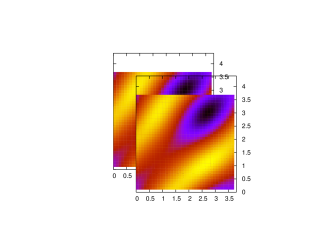
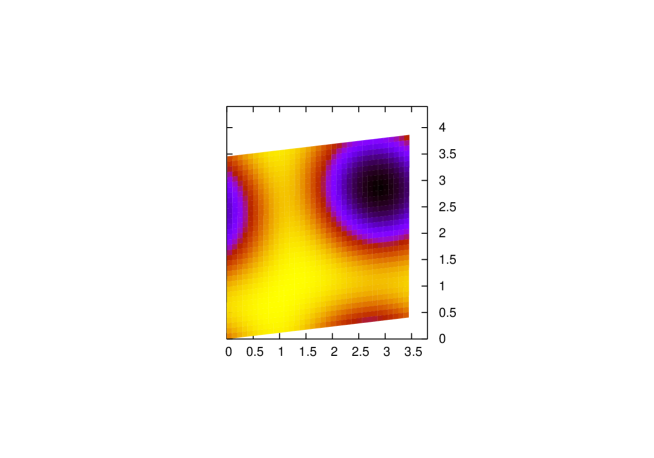
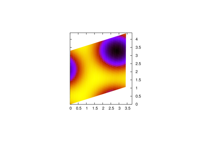
Figure 2: Transformation of a square cell under zero external stress, when the melt is quenched into the stability region of the cylindrical phase ($\chi N=15.9$, $f=0.64$).

Figure 3: Free energies (per chain) of the lamellar (solid) and cylindrical (dashed) phases under zero tension, as a function of $\chi N$, for a diblock with $f=0.64$.

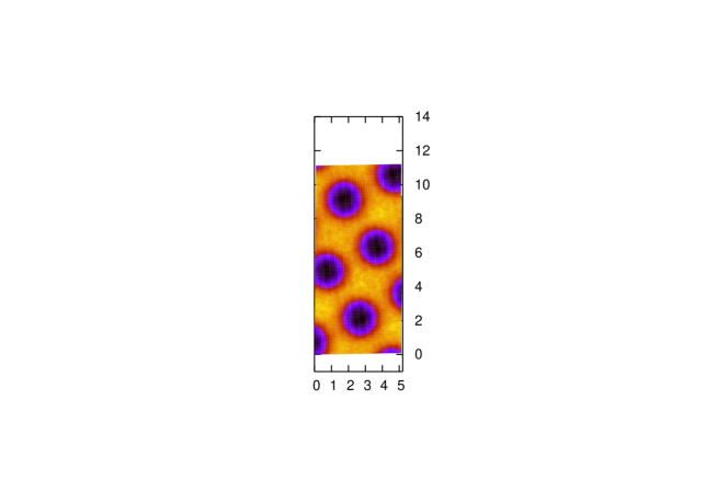
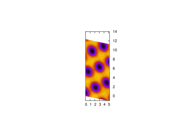
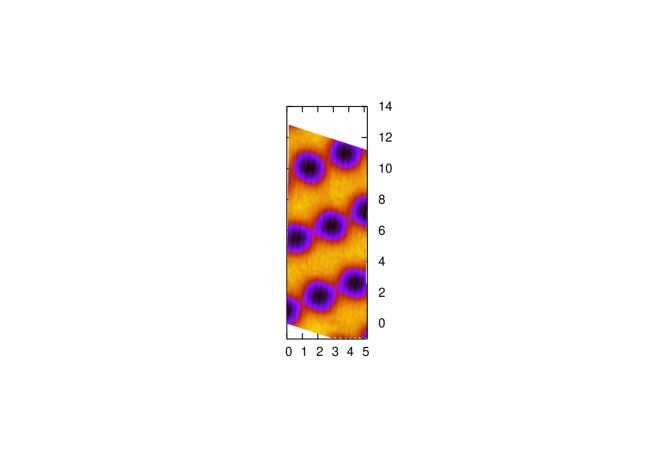
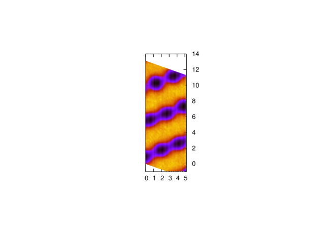
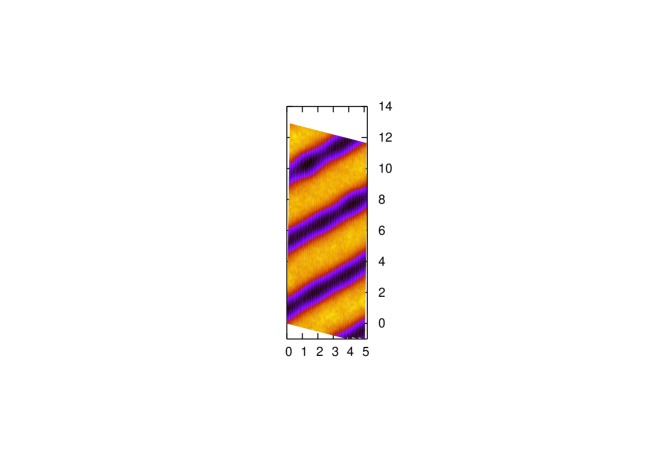
Figure 4: Six stages of the cylindrical-lamellar transformation upon compression of a cylindrical phase at $\chi N=16$ along the horizontal axis ($\sigma_{xx}-\sigma_{yy}=1$).

References

- [1] D. Frenkel and B. Smit, Understanding Molecular Simulation (Academic, New York, 1996)
- [2] M. Parrinello and A. Rahman, J. Appl. Phys. 52, 7182 (1981)
- [3] J. R. Ray and A. Rahman, J. Chem. Phys. 80, 4423 (1984)
- [4] T.H.K. Barron, M.L. Klein, Proc. Phys. Soc. 65, 523 (1965)
- [5] I. Souza, J.L. Martins, Phys. Rev B 55, 8733 (1997)
- [6] R. Marton k, A. Laio, M. Parrinello, Phys. Rev. Lett. 90, 075503 (2003)
- [7] J. I. McKechnie, R. N. Haward, D. Brown, J. H. R. Clarke, Macromolecules, 26, 198 (1993)
- [8] G.H. Fredrickson, V. Ganesan, and F. Drolet, Macromolecules, 35, 16 (2002)
- [9] F. Schmid, J. Phys.: Condens. Matter 10, 8105 (1998)
- [10] M.W. Matsen, M. Schick, Phys. Rev. Lett, 72, 2660 (1994)
- [11] S.W. Sides, G.H. Fredrickson, Polymer, 44, 5859 (2003)
- [12] F. Drolet, G.H. Fredrickson, Phys. Rev. Lett, 83, 4317 (1999)
- [13] N.M. Maurits, J.G.E.M. Fraaije, J. Chem. Phys., 107, 5879 (1997)
- [14] M.W. Matsen, J. Chem. Phys, 106, 7781 (1997)
- [15] C.A. Tyler, D.C. Morse, Macromolecules 36, 8184 (2003).
- [16] C.A. Tyler, D.C. Morse, Macromolecules 36, 3764 (2003).
- [17] R. B. Thompson, K. . Rasmussen, T. Lookman J. Chem. Phys. 101, 3990 (2004)
- [18] L. Landau, E.M. Lifschitz, Theory of Elasticity (Pergamon Press, New-York, 1986)
- [19] D. Wallace, Thermodynamics of crystals (Wiley, New-York 1973)
- [20] K.O. Rasmussen and G. Kalosakas, J. Polym. Sci., Part B: Polym. Phys. 40, 1777 (2002).
- [21] G.H. Fredrickson and S.W. Sides, Macromolecules 36, 5415 (2003).
- [22] M. Doi, S.F. Edwards, The Theory of Polymer Dynamics (Oxford University Press, Oxford, 1988)
- [23] G.H. Fredrickson, J. Chem. Phys, 117, 6810 (2002)
- [24] Z.G. Wang, J. Chem. Phys. 100, 2298 (1993)