Spontaneous spin polarization in doped semiconductor quantum wells

Abstract

We calculate the critical density of the zero-temperature, first-order ferromagnetic phase transition in $n$-doped GaAs/AlGaAs quantum wells. We find that the existence of the ferromagnetic transition is dependent upon the choice of well width. We demonstrate rigorously that this dependence is governed by the interplay between different components of the exchange interaction and that there exists an upper limit for the well width beyond which there is no transition. We predict that some narrow quantum wells could exhibit this transition at electron densities lower than the ones that have been considered experimentally thus far. We use a screened Hartree-Fock approximation with a polarization-dependent effective mass, which is adjusted to match the critical density predicted by Monte Carlo calculations for the two-dimensional electron gas.

I Introduction

The interacting electron gas is one of the fundamental systems of physics. However, in spite of a long tradition of study, the subject still has many open basic questions. Notably, the issue of the existence of a ferromagnetic transition at low density has not been settled bloch . Coulomb correlations play a central role in the low-density regime, and taking them into account theoretically (i.e., going beyond Hartree-Fock) is unfortunately notoriously difficult. This problem has been most reliably tackled with numerically intensive Monte Carlo (MC) techniques ceper ; tancep ; att ; ortiz . For the two-dimensional electron gas (2DEG), MC calculations indicate that, at $T=0$, a first-order phase transition takes place at a certain critical value $r_{sc}$ of the dimensionless average separation between electrons $r_{s}\equiv 1/\sqrt{\pi N_{s}}a^{*}_{B}$, where $N_{s}$ is the surface density and $a^{*}_{B}$ is the effective Bohr radius in the embedding medium ($a^{*}_{B}=98.7$Å for GaAs).

The most widely used methods in MC calculations foulkes are the variational Monte Carlo (VMC), which predicts ceper ; tancep a first-order phase transition at $r_{sc}=13\pm 2$ ($N_{sc}=1.9\times 10^{9}$cm^-2), and fixed-node diffusion Monte Carlo (FN-DMC) with which $r_{sc}=25$ ($N_{sc}=5.2\times 10^{8}$cm^-2) has been found att . The VMC method uses a stochastic integration to evaluate the ground-state energy for a given trial wave function. The other method, which provides lower and more accurate ground-state energies, uses a projection technique to enhance the ground-state component of a trial wave function. In addition, in the FN-DMC method implemented in reference att , backflow correlations kwon are included in the Slater determinant of the trial wave function, i.e. correlations are taken into account at the starting point of the process, for each polarization.

Of course, the ideal, purely two-dimensional electron gas cannot exist in nature. Instead, experimentally one studies quasi-two-dimensional electron gases (quasi-2DEG) like the ones formed in modulation-doped semiconductor quantum wells (QWs) ando . To the best of our knowledge, no Monte Carlo studies comparable to the ones mentioned above have been done for quasi-2DEG, but the ferromagnetic transition in QWs has been studied theoretically in the frame of the local-spin-density approximation tamb . The critical densities predicted with that technique exceed by far the density interval given by MC for the 2DEG.

On the experimental front, the spin susceptibility has recently been measured in GaAs/AlGaAs superlattices zhu , with electron densities as low as $1.7\times 10^{9}$cm^-2. In spite of the fact that this value falls into the density range predicted for a transition by the 2DEG-MC calculations, no transition was observed.

In this work, we study theoretically the possibility of a first-order transition at $T=0$ for the quasi-2DEG confined in GaAs/AlGaAs QWs as a function of the well width. We find that the width and the depth of the well play a crucial role in the existence of the transition. We prove rigorously the origin of the pronounced dependence of the transition density on the well width and predict the existence of an upper limit for this parameter beyond which the polarized phase is energetically unfavorable. We find that the transition should happen at electron densities lower than those attained experimentally so far zhu , for an optimum value of the well width, which we provide below. In our calculations we use a screened Hartree-Fock approximation scheme that includes a polarization-dependent effective mass which is introduced in order to take into account more accurately the effects of Coulomb correlation inside the well. This novel approach has the virtue of allowing us to use the results of the existing numerical Monte Carlo studies in two dimensions and extend them in a reliable way to quasi-2DEG systems.

The paper is organized as follows. In Section II.1 we introduce the basic scheme of the screened Hartree-Fock approximation and obtain the equations for the ground-state energies for the 2DEG and the quasi-2DEG. In Section II.2 we discuss the results of this approximation. In Section III we describe the polarization-dependent effective-mass approximation and we use it in combination with the available 2DEG Monte Carlo data to make predictions for QWs. We end in Section IV with a summary of our conclusions.

II Screened-Hartree-Fock theory with polarization-independent effective mass

II.1 Formalism

In a quasi-2DEG, the HF equation may be written as pk

$$\left[E_{n}^{(\zeta)}(k)-\frac{\hbar^{2}k^{2}}{2m_{b}^{\ast}}\right]\Phi_{nk}^{(\zeta)}(z)=$$ (1)

$$\left[-\frac{\hbar^{2}}{2m_{b}^{\ast}}\frac{d^{2}}{dz^{2}}+V_{ext}(z)+V_{sc}^{(\zeta)}(z)\right]\Phi_{nk}^{(\zeta)}(z)$$

$$-\frac{2\pi e^{2}}{\varepsilon}\frac{1}{A}\int dz^{\prime}\sum_{n^{\prime}occup.}\sum_{|\textbf{k}^{\prime}|<k^{(\zeta)}_{Fn^{\prime}}}\frac{e^{-|\textbf{k}-\textbf{k}^{\prime}||z-z^{\prime}|}}{|\textbf{k}-\textbf{k}^{\prime}|}$$

$$\times\Phi^{(\zeta)\ast}_{n^{\prime}k^{\prime}}(z^{\prime})\Phi_{nk}^{(\zeta)}(z^{\prime})\Phi_{n^{\prime}k^{\prime}}^{(\zeta)}(z),$$

where $\Phi_{nk}^{(\zeta)}(z)$ are the $n$th subband eigenstates and $E_{n}^{(\zeta)}(k)$ the corresponding eigenenergies, $m_{b}^{\ast}=0.067m_{e}$ is the effective mass ($m_{e}$ being the electron rest mass), $\varepsilon=12.5$ is the dielectric constant, $e$ is the electron charge, $A$ is the crystal area, and k is the in-plane wave vector. In all our calculations we take the z-axis as the growth direction of the heterostructure. The self-consistent potential $V_{sc}^{(\zeta)}(z)$ is obtained by integration of the Poisson equation and is expressed as

$$V^{(\zeta)}_{sc}(z)=-\frac{4\pi e^{2}}{\varepsilon}\left(\int_{0}^{z}dz^{\prime}(z-z^{\prime})n^{(\zeta)}(z^{\prime})-\frac{N_{s}}{2}z\right),$$ (2)

where the $\zeta$-dependent electron density is

$$n^{(\zeta)}(z)=\frac{2-\zeta}{2\pi}\sum_{n\ occup.}\int_{0}^{k^{(\zeta)}_{Fn}}kdk|\Phi^{(\zeta)}_{n}(z,k)|^{2}.$$ (3)

Here, $N_{s}$ is the doping sheet density and the external potential $V_{ext}(z)$ is the sum of the confinement potential of the heterostructure plus the electrostatic potential generated by the ionized donors (located symmetrically). The Fermi level $k_{Fn}^{(\zeta)}$ for each subband satisfies $2\pi(1+\zeta)N_{s}=\sum_{n}k_{Fn}^{(\zeta)2}$. The spin polarization index only takes the values $\zeta=0$ and $\zeta=1$ since, at $T=0$, no stable partially-polarized phases are possible in 2DEG att ; dha1 . In contrast, recent calculations in 3DEG show that the transition is not of first order, but rather a continuous one involving partial spin-polarization states ortiz . Here we make the hypothesis that the quasi-2DEG behaves like the 2DEG provided that the well width remains sufficiently small.

We solve equation (1) following a method similar to that developed in reference pk . We expand the eigenfunctions $\Phi_{nk}^{(\zeta)}(z)$ in the single-electron QW-basis functions $\{\phi_{n}(z),\epsilon_{n}\}$, i.e.

$$\Phi_{nk}^{(\zeta)}(z)=\sum_{p}a_{pn}^{(\zeta)}(k)\phi_{p}(z).$$ (4)

This enables us to write the eigenvalue equation

$$\hat{H}^{(\zeta)}(k)\vec{b}_{n}^{(\zeta)}(k)=E_{n}^{(\zeta)}(k)\vec{b}_{n}^{(\zeta)}(k),$$ (5)

with $\vec{b}_{n}^{(\zeta)}(k)=(a_{1n}^{(\zeta)}(k),...,a_{pn}^{(\zeta)}(k),...)^{T}$. The matrix elements of the Hamiltonian operator $\hat{H}^{(\zeta)}(k)$ are

$$H_{tp}^{(\zeta)}(k)=\left[\epsilon_{p}+\frac{\hbar^{2}k^{2}}{2m_{b}^{\ast}}\right]\delta_{tp}+\langle\phi_{t}|V_{sc}^{(\zeta)}|\phi_{p}\rangle$$

$$-V^{(1)(\zeta)}_{tp}(k)-V^{(2)(\zeta)}_{tp}(k),$$ (6)

$$V^{(1)(\zeta)}_{tp}(k)=\frac{e^{2}}{\varepsilon}\sum_{n^{\prime}}\int_{0}^{k^{(\zeta)}_{Fn^{\prime}}}k^{\prime}dk^{\prime}\sum_{qr}G_{tr,qp}(k,k^{\prime})$$

$$\times a_{qn^{\prime}}^{(\zeta)}(k^{\prime})a_{rn^{\prime}}^{(\zeta)}(k^{\prime}),$$ (7)

$$V_{tp}^{(2)(\zeta)}(k)=\frac{e^{2}}{\varepsilon}\sum_{n^{\prime}}\int_{0}^{k^{(\zeta)}_{Fn^{\prime}}}k^{\prime}dk^{\prime}a_{pn^{\prime}}^{(\zeta)}(k^{\prime})a_{tn^{\prime}}^{(\zeta)}(k^{\prime})$$

$$\times\frac{2}{\pi}\int_{0}^{\pi/2}\frac{d\varphi}{\sqrt{(k+k^{\prime})^{2}-4kk^{\prime}\sin^{2}\varphi}+q^{(\zeta)}_{s}},$$ (8)

$$G_{tr,qp}(k,k^{\prime})=\int\int dzdz^{\prime}\phi^{\ast}_{t}(z)\phi_{r}(z)\phi^{\ast}_{q}(z^{\prime})\phi_{p}(z^{\prime})$$

$$\times\int_{0}^{2\pi}\frac{d\varphi}{2\pi}\frac{e^{-|\textbf{k}-\textbf{k'}||z-z^{\prime}|}-1}{|\textbf{k}-\textbf{k'}|}.$$ (9)

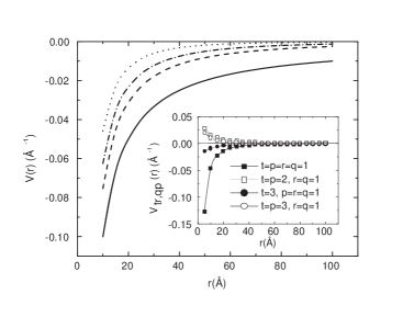
Figure 1: Different Coulomb potentials. The solid line corresponds to the unscreened Coulomb potential $V(r)=1/r$. The dashed (dot-dashed) curve corresponds to the Thomas-Fermi screened Coulomb potential for the polarized (unpolarized) case. The dotted curve represents the potential $V(r,d_{W})$, Fourier transform of equation (9) (with respect to $q=|\textbf{k}-\textbf{k'}|$) for an infinite QW of $d_{W}=100$Å, for $t=r=q=p=1$. Inset: the Fourier transform of equation (9) for an infinite QW of $d_{W}=100$Å for different values of $t,r,q,p$.

We note that equations from reference pk have a number of misprints which are corrected here com1 .

To introduce screening in the HF approximation we note from equations (7) and (8) that $V^{(2)(\zeta)}_{tp}(k)$ is the only term present in the pure 2D case and describes the long-range in-plane Coulomb interaction. Thus, we have dressed the interaction line of the exchange diagram mano by replacing the bare Coulomb potential $V(q=|\textbf{k}-\textbf{k'}|)=(2\pi e^{2}/\varepsilon)(1/q)$ in equation (8) with the statically screened Coulomb potential

$$V^{(\zeta)}_{s}(q)=\frac{2\pi e^{2}}{\varepsilon}\frac{1}{q+q^{(\zeta)}_{s}},$$ (10)

where $q^{(\zeta)}_{s}=(2-\zeta)/a^{\ast}_{B}$ is the $\zeta$-dependent Thomas-Fermi wave number for the 2DEG. Unfortunately, the Fourier transform in 2D real space of equation (10) cannot be obtained analytically but its decay at large $r$ is found to be davies

$$V_{s}^{(\zeta)}(r)=\frac{e^{2}}{\varepsilon}\frac{1}{q^{2(\zeta)}_{s}r^{3}}.$$ (11)

On the other hand, $V^{(1)(\zeta)}_{tp}(k)$ (Eq. (7)) which arises from the intrinsic inhomogeneity of charge distribution in a quasi-2DEG, represents an interaction of short range. To see this, we consider the Fourier transform in 2D real space

$$V(r,|z-z^{\prime}|)=\frac{e^{2}}{\varepsilon}\left(\frac{1}{\sqrt{r^{2}+|z-z^{\prime}|^{2}}}-\frac{1}{r}\right),$$ (12)

of the potential $V(q,z-z^{\prime})=(2\pi e^{2}/\varepsilon)(e^{-q|z-z^{\prime}|}-1)/q$ contained in equation (9). It can be shown that $V(r,|z-z^{\prime}|)$ is of short range in the plane vasko and that at large $r$ it can be approximated as

$$V(r,d_{W})=-0.032\frac{e^{2}}{\varepsilon}\frac{d^{2}_{W}}{r^{3}},$$ (13)

where we calculate the $z$ and $z^{\prime}$ integration of $|z-z^{\prime}|^{2}$ for an infinite QW of well width $d_{W}$ setting the subband indexes equal to one. From equations (11) and (13) we note that both potentials decay at the same rate at large $r$ and that $V(r,d_{W})\approx 0.128V_{s}^{(0)}(r)$ and $V(r,d_{W})\approx 0.032V_{s}^{(1)}(r)$ for $d_{W}=a^{*}_{B}$.

We show in Figure 1 that the potential defined by equation (12), suitably integrated over $z$ and $z^{\prime}$ (dotted line), has a range that is shorter than the range of the Thomas-Fermi screened Coulomb potential for the polarized (dashed line) and unpolarized (dot-dashed line) cases, for $t=r=q=p=1$. In the inset we show that this case dominates over all others (we only show a few relevant examples).

In what follows we assume that only the first subband is occupied, and therefore the summations over the subband index may be omitted.

In solving the eigenvalue equation by iteration, we consider that self-consistency is achieved at the $l$th step when $|a^{(\zeta)(l)}_{pn}(k)-a^{(\zeta)(l-1)}_{pn}(k)|/|a^{(\zeta)(l-1)}_{pn}(k)|<10^{-4}$ for all $p,n$ and $k$. We obtain the set of eigenfunctions and eigenenergies $\{\Phi^{(\zeta)}_{nk}(z),E^{(\zeta)}_{n}(k)\}$ for $\zeta=0$ and $\zeta=1$, which allows us to write the ground-state energy per particle

$$E^{(\zeta)}_{HF}=\frac{2-\zeta}{4\pi N_{s}}\int_{0}^{k^{(\zeta)}_{F}}kdk\left[E^{(\zeta)}_{1}(k)+\tilde{\epsilon}^{(\zeta)}_{1}(k)+\frac{\hbar^{2}k^{2}}{2m_{b}^{\ast}}\right],$$ (14)

with

$$\tilde{\epsilon}^{(\zeta)}_{1}(k)=\sum_{n}\epsilon_{n}|a^{(\zeta)}_{n1}(k)|^{2}.$$ (15)

In order to check our quasi-2DEG calculations in QWs when $d_{W}$ tends to zero, we shall compare our results to the 2DEG screened HF case fw

$$E^{(\zeta)}_{HF2D}=\frac{e^{2}}{2a^{\ast}_{B}\varepsilon}\left\{\frac{1+\zeta}{r_{s}^{2}}-\frac{4}{\pi r_{s}}[2\zeta+\sqrt{2}(1-\zeta)]\textbf{I}(x_{\zeta})\right\},$$ (16)

where $x_{\zeta}=\frac{1}{4}[\zeta+2\sqrt{2}(1-\zeta)]r_{s}$ is the polarization-dependent Thomas-Fermi wave number divided by $2k^{(\zeta)}_{F}$ and

$$\textbf{I}(x_{\zeta})=\int_{0}^{1}\frac{xdx}{x+x_{\zeta}}[\arccos(x)-x\sqrt{1-x^{2}}].$$ (17)

II.2 Results

In this section we present the results obtained with the screened Hartree-Fock approximation with polarization-independent effective masses introduced in the previous section.

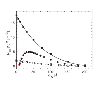
Figure 2: Well-width dependence of the critical density in the screened HF approximation. Solid squares correspond to infinite quantum wells and solid circles to finite QWs with well height $V_{b}$=247 meV. Open squares correspond to infinite QWs with polarization-dependent effective masses with a constant ratio $f\equiv m^{\ast}_{1}/m^{\ast}_{0}=0.65$. The solid and dashed lines are obtained with equations (24) and (27) (with $f=0.65$), respectively, for infinite QWs.

In Figure 2, we plot the critical density for infinite QWs (in which there is no barrier penetration) in the screened HF approximation as a function of well width $d_{W}$ (solid squares). The limiting point at $d_{W}=0$ (2DEG) was calculated with equation (16) and the remaining points with equation (14). The excellent match between these two different equations reflects the correctness of our derivations and calculations com1 . We see that the critical density for the infinite QWs is a rapidly decreasing function of $d_{W}$. This result, which looks superficially correct on the basis of a gradual 2D to 3D transition, can be explained rigorously in terms of the interplay between different components of the exchange interaction in a quasi-2DEG, as follows. We found that the coefficients $a^{(\zeta)}_{p1}(k)$ (Eq. (4)) change very little with $k$ and $a^{(\zeta)}_{11}(k)\approx 1$ whereas $a^{(\zeta)}_{p1}(k)\ll 1$ for $p>1$. This result is a direct consequence of the small-density condition since, if this condition is met, the ground-state wave function must retain the shape of its one-electron counterpart in a QW. Thus, $V_{11}^{(2)(\zeta)}(k)$ (Eq. (8)) is positive and it is the leading matrix element, yielding a negative (see Eq. (6)) and $d_{W}$-independent contribution to the exchange energy (pure 2D case). In contrast, the matrix elements $V^{(1)(\zeta)}_{tp}(k)$ are slowly varying functions of $k$ since we are studying small-width and low-density heterostructures. If these conditions are fulfilled, we can expand the exponential in equation (9) up to first order since the exponent satisfies the following inequality:

$$|\textbf{k}-\textbf{k'}||z-z^{\prime}|\leq 2k^{(\zeta)}_{F}d_{W}=2\sqrt{2(1+\zeta)}\frac{1}{r_{s}}\frac{d_{W}}{a^{*}_{B}}\leq 0.3,$$ (18)

provided that $r_{s}\geq 13$ (lower MC limit for the transition) and the well width $d_{W}\leq a^{*}_{B}$ ($=98.7$Å). Then we perform the integration over $z$ and $z^{\prime}$ (infinite QWs) yielding $G_{11,11}=-0.207d_{W}$. Thus, $V_{11}^{(1)(\zeta)}$ is negative, proportional to $d_{W}$ and $k$-independent. The matrix elements $V_{tp}^{(1)(\zeta)}$ for indices with opposite parity are always zero since due to the symmetry of the wave functions we have $G_{t1,1p}=0$. On the other hand, we have evaluated $G_{t1,1p}$ for indices with equal parity obtaining that these are considerably smaller than $G_{11,11}$ rendering $V_{tp}^{(1)(\zeta)}$ practically diagonal. Also, $\langle\phi_{t}|V_{sc}^{(\zeta)}|\phi_{p}\rangle\approx 0$ (see Eq. (6)) for the non-diagonal elements since, due to the low-density condition, $V_{sc}^{(\zeta)}$ must be a very slowly varying function of $z$. Thus, $H_{tp}^{(\zeta)}(k)$ is almost diagonal, being its first eigenenergy

$$E^{(\zeta)}_{1}(k)\approx\epsilon_{1}+\frac{\hbar^{2}k^{2}}{2m_{b}^{\ast}}+\langle\phi_{1}|V^{(\zeta)}_{sc}|\phi_{1}\rangle-V^{(1)(\zeta)}_{11}-V^{(2)(\zeta)}_{11}(k).$$ (19)

With this expression for $E^{(\zeta)}_{1}(k)$ we can obtain an approximate equation for $N_{sc}$. We only need to make two easily justified additional approximations. From the behavior of the coefficients $a^{(\zeta)}_{p1}(k)$, i.e. $a^{(1)}_{11}(k)\approx a^{(0)}_{11}(k)\approx 1$ and $a^{(1)}_{p1}(k)\approx a^{(0)}_{p1}(k)\approx 0$ for $p>1$ it can be seen (from Eq. (15)) that $\tilde{\epsilon}^{(\zeta)}_{1}(k)\approx\epsilon_{1}$ and (from Eq. (4)) $\Phi^{(\zeta)}_{1k}(z)\approx\phi_{1}(z)$. Using the latter in equation (3) we get $n^{(\zeta)}(z)\approx(2-\zeta)(1+\zeta)N_{s}\phi^{2}_{1}(z)/2=N_{s}\phi^{2}_{1}(z)$, and therefore a $\zeta$-independent $\langle\phi_{1}|V_{sc}|\phi_{1}\rangle$ (see Eq. (2)). By inserting equation (19) in equation (14) we obtain, after some algebra, the following equation for the energy shift between both phases

$$E^{(1)}_{HF}-E^{(0)}_{HF}\approx\frac{\pi N_{s}e^{2}a^{*}_{B}}{2\varepsilon}\left[1+0.207\frac{d_{W}}{a^{*}_{B}}-4F(N_{s})\right],$$ (20)

where

$$F(N_{sc})=\int_{0}^{1}xdx\int_{0}^{1}x^{\prime}dx^{\prime}$$

$$\times\frac{2}{\pi}\int_{0}^{\pi/2}d\varphi[g_{1}(N_{sc},x,x^{\prime},\varphi)$$

$$-g_{0}(N_{sc},x,x^{\prime},\varphi)],$$ (21)

with

$$g_{0}(N_{sc},x,x^{\prime},\varphi)=\left[\sqrt{2\pi N_{sc}}a^{*}_{B}\right.$$

$$\left.\times\sqrt{(x+x^{\prime})^{2}-4xx^{\prime}sin^{2}\varphi}+2\right]^{-1},$$ (22)

and

$$g_{1}(N_{sc},x,x^{\prime},\varphi)=\left[\sqrt{\pi N_{sc}}a^{*}_{B}\right.$$

$$\left.\times\sqrt{(x+x^{\prime})^{2}-4xx^{\prime}sin^{2}\varphi}+q^{(1)}_{s}/q^{(0)}_{s}\right]^{-1},$$ (23)

where $x\equiv k/k^{(0)}_{F}$ in $g_{0}$ and $x\equiv k/k^{(1)}_{F}$ in $g_{1}$. The same holds for $x^{\prime}$ and $k^{\prime}$.

Taking into account that the energy shift $E^{(1)}_{HF}-E^{(0)}_{HF}$ must be zero at the transition density, we may write the following equation that relates $d_{W}$ and $N_{sc}$

$$1+0.207\frac{d_{W}}{a^{*}_{B}}=4F(N_{sc}).$$ (24)

Finally, to demonstrate that the transition density is a decreasing function of the well width, we need to prove that $F(N_{sc})$ is also a decreasing function. To see this, we note firstly that $g_{1}>g_{0}$ for all values of its arguments making the function $F(N_{sc})$ always positive allowing equation (24) to be solvable. Secondly, both $g_{0}$ and $g_{1}$ are decreasing functions of $N_{sc}$ for all values of $x,x^{\prime},\varphi$ and it is straightforward to prove that $g_{1}$ decreases more rapidly than $g_{0}$ making $F(N_{sc})$ a decreasing function. Thus, an increase of $d_{W}$ must be accompanied with a decrease of $N_{sc}$ proving that the monotonically decreasing dependence of $N_{sc}$ on $d_{W}$ is governed by the competing action of the different components of the exchange interaction: the in-plane component represented by $F(N_{sc})$ and the out-of-plane term driven by $d_{W}$. The behavior of $g_{0}$, $g_{1}$ and $F$ that we described can also be recognized in the unscreened HF case indicating that the dependence of $N_{sc}$ on $d_{W}$ is purely due to exchange. The validity of our approximation can be verified in Figure 2 where the solutions of equation (24) are depicted with the solid line. This curve approaches very well the exact values (solid squares) indicating that the approximations we made to derive it are well justified. For low densities (high $r_{s}$) and low well widths, the solid curve fits excellently the solid squares since in these regimes the approximations we made become exact. In the intermediate region ($d_{W}\approx 100$Å) the solid curve fits very well the solid squares.

A look at equation (24) also indicates that there exists an upper limit for the well width. In fact, due to the decrease of $F(N_{sc})$ and since $F(0)$ is finite, it can be seen from equations (22) and (23) that the following relation holds

$$0.207\frac{d_{WL}}{a^{*}_{B}}=\frac{q^{(0)}_{s}}{q^{(1)}_{s}}-\frac{3}{2}.$$ (25)

Thus, it must be $d_{W}<d_{WL}=2.42a^{*}_{B}\approx 239$Å to allow the confined electrons to reach the polarized phase. This new result is entirely due to the Thomas-Fermi screening and is not present in the unscreened HF approximation since $F(0)$ diverges in this case. Furthermore, the ratio of the Thomas-Fermi wave numbers for both polarizations must be $q^{(0)}_{s}/q^{(1)}_{s}>3/2$ (in our case it is $q^{(0)}_{s}/q^{(1)}_{s}=2$). Otherwise, no polarized state could be possible in a QW. These key results indicate that the well width plays a crucial role in the search for spontaneous spin polarization in QWs tutuc .

The implications of the existence, according to our calculations, of an upper limit for the well width must be considered with some care. If one attempts to reach a 3DEG system by increasing the well width one would apparently fall into the paradox that no transition is possible in 3DEG. This conclusion is incorrect for two reasons. First, we must take into account that the 3DEG-MC results are obtained in the jellium model, in which the positive background is taken to be a uniform neutralizing static charge distribution, whereas in our quantum-well calculations the positive charges of the ionized donors are located far away from the electron gas, which results in an important change in the direct Coulomb energy. In other words, wide-enough quantum wells and 3DEG jellium model must be considered as different systems. Secondly, our calculation assumes that only one subband is occupied (a valid assumption in narrow quantum wells at low density) whereas any extrapolation of our conclusions to 3DEG systems would have to contemplate necessarily occupation of many subbands. Thus, we reach the conclusion that the most likely scenario is that there is a phase transition in narrow quantum wells, which disappears for intermediate well widths, and reenters at wider well widths as expected when the 3DEG limit is approached.

We now use the previous result to analyze the critical density for finite QWs, plotted in Figure 2 with solid circles. We set the height of the QWs to $V_{b}=247$ meV, a typical experimental value bastard . This curve exhibits a non-monotonic dependence on the well-width showing a maximum for $d_{W}\approx 35$Å. Also we observe a general reduction of the critical density with respect to the case of infinite QWs. This can be simply understood in terms of the previous result (monotonically decreasing critical density for the infinite wells) and the penetration of the electron wave function into the AlGaAs barriers; the latter causes the wave function to spread beyond the nominal well width, effectively “enlarging” the well. As a consequence, for example, a finite QW of $d_{W}\approx 60$Å has the same critical density as that of an infinite QW of $d_{W}\approx 100$Å. In fact, the penetration depth $d_{B}=\hbar/\sqrt{2m_{b}^{\ast}(V_{b}-E_{1})}$ increases when $E_{1}$ is raised as $d_{W}$ is lowered vasko . This effect produces an inflection point at $d_{W}\approx 75$Å and the mentioned maximum at $d_{W}\approx 35$Å due to the competition between $d_{W}$ and $d_{B}$.

Let us go back to the curve for infinite QWs in Figure 2. The limiting ($d_{W}=0$) value $N_{sc}=17.5\times 10^{9}$cm^-2 corresponds to $r_{sc}=4.32$, showing a sizable increase with respect to the (unscreened) HF value $r_{sc}=2.01$ raja . This increase, however, is not sufficient if we consider the value $r_{sc}=13$ obtained in reference ceper using VMC. This indicates that a significant degree of Coulomb correlation is being left out in the screened HF approximation.

III Polarization-dependent effective masses

III.1 Two-dimensional case

In order to go further and improve our treatment of Coulomb correlation, we need an approximation scheme applicable to the quasi-2DEG such that as $d_{W}$ tends to zero (pure 2DEG) the critical density approaches the values predicted by MC calculations ceper ; tancep ; att . To achieve this, we incorporate phenomenological polarization-dependent effective masses $m_{0}^{\ast}$ (unpolarized) and $m_{1}^{\ast}$ (polarized) in our formalism. Due to the lack of experimental data on effective masses in GaAs/AlGaAs heterostructures for both polarizations and that no calculations on polarized effective masses exist in 2DEG, we resort to calculations of unpolarized effective masses and ground-state energies in pure 2DEG janmin ; krako ; ceper to justify this procedure. Let us summarize the conclusions of those studies relevant in our context:
(a) Coulomb correlation increases the effective mass krako .
(b) The absolute value of the correlation energy of the unpolarized 2DEG ground state is greater than its polarized counterpart ceper .
(c) The absolute value of the correlation energy is greater in 2D than in 3D (both unpolarized), leading to 2D effective masses substantially larger than those of the 3D case at equal $r_{s}$ janmin .
(d) The correlation-energy shift between both phases in 2D is greater than the unpolarized correlation energy shift between 2D and 3D ceper .
Making use of (a) and (b), with the supporting evidence of (c) and (d), we conclude that $m_{0}^{\ast}$ must be substantially larger than $m_{1}^{\ast}$ at equal $r_{s}$.

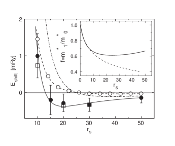
Figure 3: Ground-state energy shift $E_{shift}=E_{HF2D}^{(1)}-E_{HF2D}^{(0)}$ versus $r_{s}$. Solid circles represent the reported values in Table I of reference ceper . The error bars denote the VMC standard errors. Open squares correspond to the values tabulated in Tables I and II for the VMC method in reference tancep . No error bars are plotted for clarity. Open circles belong from reference att . The solid and dot-dashed lines represent our calculations obtained with equation (26) for polarization-dependent effective masses using $f=0.65$ and $f=0.49$ respectively. The dashed curve corresponds to the same calculations but using the values of $f$ that come from $f(r_{s})$ showed in the inset (dashed line). In the inset, solid and dashed lines correspond to the values of $f$ that fit the curves $E_{shift}$ from reference ceper and reference att respectively.

By defining the ratio $f=m^{\ast}_{1}/m^{\ast}_{0}$ and rewriting $x_{\zeta}=\frac{1}{4}[f\zeta+2\sqrt{2}(1-\zeta)]r_{s}$ we may write equation (16) as

$$E^{(\zeta)}_{HF2D}=\frac{e^{2}m_{0}^{\ast}}{2a^{\ast}_{B}\varepsilon}\left\{\frac{1+\zeta}{[(f-1)\zeta+1]r_{s}^{2}}\right.$$

$$\left.-\frac{4}{\pi r_{s}}[2\zeta+\sqrt{2}(1-\zeta)]\textbf{I}(x_{\zeta})\right\}.$$ (26)

We observe from reference janmin that $m^{\ast}_{0}\approx 1.2$ for $r_{s}>5$ in the modified Hubbard approximation. That approximation is an attempt at including correlation effects by means of the introduction of the Thomas-Fermi wave number in the so-called local-field correction factor. Since we have incorporated screening correlations and HF effects within a similar scheme, we take $m^{\ast}_{0}=1$ in equation (26) to avoid an overestimation of the effective mass in the unpolarized phase.

Using equation (26), the lowest 2DEG-VMC value, i.e. $r_{sc}=13$, is obtained with $f=0.65$. With this value of $f$ we calculate $E_{shift}=E^{(1)}_{HF2D}-E^{(0)}_{HF2D}$ and plot it versus $r_{s}$ in Figure 3 (solid line). Here we have taken $e^{2}/2a^{\ast}_{B}\varepsilon=$ 1 Ry to compare our $E_{shift}$ against MC results. The solid circles correspond to the results obtained in reference ceper and the open squares are from reference tancep . We note the excellent agreement between our curve and the MC points: by adjusting only one point our curve meets all the points obtained in reference ceper ; tancep . This agreement implies that the ratio between both effective masses depends weakly on the density and supports the validity of our assumption of a density-independent $f$ factor. This conclusion is consistent with the fact that in the modified Hubbard approximation the unpolarized effective mass is a slowly varying function for $r_{s}>5$ janmin . If this were also the behavior of the polarized effective mass, we could conclude that $f$ would be a slowly varying function of $r_{s}$.

We now repeat the previous analysis but using the data of Attaccalite et al. att . In that paper the authors obtain $r_{sc}=25$ which, as we mentioned in the introduction, is the highest value found in the literature for spontaneous spin polarization in 2DEG at zero temperature. We find that equation (26) reproduces the value $r_{sc}=25$ when $f=0.49$. In Figure 3 (dash-dotted line) we plot the energy shift, $E_{shift}=E^{(1)}_{HF2D}-E^{(0)}_{HF2D}$, versus $r_{s}$, for this value of $f$. This curve does not fit well the data from reference att shown as open circles. Instead, we find that the ratio $f$ now taken as a function of $r_{s}$ (dashed line in the inset) fits very well the MC points calculated in reference att (open circles) when it is used in equation (26) (dashed line in Fig. 3. For completeness, we show in the inset (solid line) the values of $f$ as a function of $r_{s}$ that fit the parametrization of $E_{shift}$ obtained by Ceperley ceper . This curve exhibits a weak dependence on $r_{s}$ for $r_{s}>10$ giving support to our initial assumption of a constant value $f=0.65$.

III.2 Quasi-two-dimensional case

We now apply the polarization-dependent effective-mass approximation to the quasi-2DEG by means of a slight modification in equation (1). We note that the two effective masses $m_{b}^{\ast}$ on both sides of equation (1) belong to different situations vasko : the $m_{b}^{\ast}$ on the l.h.s. represents the in-plane effective mass and therefore is being affected by Coulomb correlations. In contrast, the $m_{b}^{\ast}$ on the r.h.s. reflects the out-of-plane effective mass of one electron moving in the z-direction governed mainly by $V_{ext}(z)$ and $V_{sc}^{(\zeta)}(z)$, and thus not being affected by Coulomb correlations, according to our discussion about screening in Section II.1. Then we solve the eigenvalue equation, equation (1), and use equation (14) for both polarizations incorporating the effective masses $m^{\ast}_{0}=m^{\ast}_{b}$ and $m^{\ast}_{1}=fm^{\ast}_{b}$ (the last one only in the in-plane terms). We plot in Figure 2, with open squares, the results obtained for infinite QWs for $f=0.65$. We calculate the limiting point at $d_{W}=0$ with equation (26) and the remaining points with equation (14) with the above-mentioned replacement giving an excellent match. We show in the Figure 4, in a logarithmic scale for the vertical axis, the results for finite QWs (open circles) and infinite QWs (open squares) where we have taken $f=0.65$. Both curves exhibit the same general characteristics as in Figure 2 (solid squares and solid circles).

Now we obtain an equivalent of equation (24) by incorporating the ratio $f$ that multiplies the band mass $m^{*}_{b}$ for the polarized phase, yielding

$$\frac{2}{f}-1+0.207\frac{d_{W}}{a^{*}_{B}}=4F(N_{sc},f),$$ (27)

where $F(N_{sc},f)$ is the same as in equation (21), but $g_{1}$ now reads

$$g_{1}(N_{sc},x,x^{\prime},\varphi)=\left[\sqrt{\pi N_{sc}}a^{*}_{B}\right.$$

$$\left.\times\sqrt{(x+x^{\prime})^{2}-4xx^{\prime}sin^{2}\varphi}+fq^{(1)}_{s}/q^{(0)}_{s}\right]^{-1}.$$ (28)

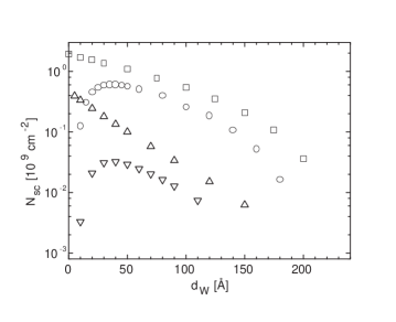
Figure 4: Well-width dependence of the critical density in the screened HF approximation with polarization-dependent effective masses. Open squares (circles) correspond to infinite (finite) QWs with a constant ratio $f\equiv m^{\ast}_{1}/m^{\ast}_{0}=0.65$. Up (down) triangles correspond to infinite (finite) QWs for a ratio $f$ which depends on $r_{s}$ (dashed line in the inset of Fig. 3).

The polarization-dependent effective-mass approximation does not change the previous result regarding the monotonically decreasing dependence of $N_{sc}$ on $d_{W}$ since $f<1$. We show that the solutions of the approximate equation (27) (dashed curve) depicted in Figure 2 for $f=0.65$, fit perfectly the exact values (open squares). We observe that since $F(0,f)=\frac{1}{4}(\frac{2}{f}-\frac{1}{2})$, $d_{WL}$ does not depend on $f$ (see Eq. (27)). Thus, $d_{WL}$ depends on correlations, in our Thomas-Fermi model, via the ratio $q^{(0)}_{s}/q^{(1)}_{s}$ and, consequently, the relation $d_{WL}=2.42a^{*}_{B}$ is a universal one, i.e. it holds for QWs of any material. We note that this interesting result does not depend on the approximations we made to derive equation (27) since those become exact as $N_{s}$ tends to zero.

On the other hand, the location of the observed maximum remains unchanged with respect to the $f=1$ case (solid circles in Fig. 2) in accordance to our initial assumption that screening and correlations manifest only in the plane. Up (down) triangles correspond to infinite (finite) QWs where we have taken the ratio $f$ as the dashed curve in the inset of Figure 3 (Attaccalite et al. att ). We observe a drastic diminution of the transition densities in this case for both infinite and finite QWs. We note that the MC density interval for spontaneous spin polarization mentioned in Section I, appears notoriously shrunk for the finite QWs studied here. In fact, from Figure 4 we obtain a new density interval for the transition densities in finite QWs between $N_{sc}=3.2\times 10^{7}$cm^-2 and $N_{sc}=6.1\times 10^{8}$cm^-2. We take these values from the transition densities at the maximum of the curves related to FN-DMC (down triangles) and VMC (open circles) respectively.

In reference zhu , the spin susceptibility ($=m^{\ast}g^{\ast}$) has been measured in a high quality 200-fold GaAs/AlGaAs superlattice of 100Å of GaAs wells and 30Å barriers of Al_0.32Ga_0.68As, with unprecedented low densities such as $N_{s}=1.7\times 10^{9}\mbox{cm}^{-2}$ ($r_{s}=13.9$) and no transition was observed. According to what we have mentioned above, this is not surprising. There are several possible reasons for this negative result. We first note that the density used, although low enough for a transition in the pure 2DEG, is clearly too high considering the finite well width for finite QWs: for $d_{W}=100$Å (Fig. 4), the electron density achieved in reference zhu is 6.5 times higher than our critical density (open circles) which uses the ratio $f$ that matches the 2DEG value from reference ceper and 50 times higher than the critical density (down triangles) which uses the $r_{s}$-dependent ratio $f$ that matches the 2DEG energy shifts $E_{shift}$ from reference att . Also, due to the tunneling of the electrons into the AlGaAs barriers, the superlattice acts like a single, extremely wide QW. Furthermore, it is possible that if the QW were sufficiently wide, the quasi-2DEG could lose its two-dimensional characteristics, allowing for stable partially-polarized phases like those possible in the 3DEG, turning more difficult the detection of the transition. We note that the effects of in-plane correlations combined with the finite well widths and heights of QWs produce a drastic diminution of the transition densities by a factor that ranges from 3 to 15 depending on which method VMC or FN-DMC turns out to be the best tool to estimate the transition density in pure 2DEG. For the best case, it should become necessary to achieve electron densities lower that the ones studied experimentally thus far by a factor of 3 and by a factor of 53 in the worst case. Very different could be the quasi-two-dimensional hole gas (quasi-2DHG) scenario since in that system, high $r_{s}$ values such as $r_{s}\approx 80$ are already attainable noh . However, our theoretical predictions about the critical transition density in n-doped GaAs/AlGaAs QWs cannot be straightforwardly translated to quasi-2DHG. The adaptation of our formalism to the problem with holes is currently in progress.

Based on the insight gained from our calculations, we propose that the optimal conditions for observing a ferromagnetic transition in multiple QWs are:
(a) well widths between $30$Å and $50$Å 
(b) wide AlGaAs barriers between wells to prevent tunneling, and
(c) well height $V_{b}$ as large as possible to minimize barrier-penetration effects.

In a recent experimental work, Gosh et al. ghosh report a possible spontaneous spin polarization in mesoscopic two-dimensional systems that is at odds with our findings. They have used 2DEGs in Si $\delta$-doped GaAs/AlGaAs heterostructures with densities as low as $N_{s}=5\times 10^{9}$cm^-2 ($r_{s}=7.6$) and the temperature was set at $T=40$ mK or equivalently $T/T_{F}\approx 0.02$ since $T_{F}=2.3$ K at $r_{s}=7.6$. Somewhat surprisingly, according to their interpretation of the data, these authors found partial spin polarization with $\zeta=0.2$. The authors attribute this partial spin polarization to the finite $T$ since no partial spin polarization is possible in 2DEG at $T=0$ att ; dha1 . However, in reference dha1 the authors find partial spin polarization for $T/T_{F}$ between 0.3 and 1.6, i.e. well above $T/T_{F}=0.02$ reported in reference ghosh . On the other hand, $r_{s}=7.6$ is considerably lower than the lowest value for spin polarization in 2DEG ceper .

IV Summary

In summary, we have calculated the ferromagnetic critical density at $T=0$ of the quasi-two-dimensional electron gas confined in semiconductor GaAs-based symmetrically-doped quantum wells. We use the screened Hartree-Fock approximation and prove rigorously that the pronounced decrease of the transition density with the well width is governed by the interplay between the in-plane and the out-of-plane components of the exchange interaction. The combination of these exchange terms with the Thomas-Fermi screening produces a universal upper value for the well width beyond which the polarized state cannot exist. We add different effective masses for both spin polarizations, which are introduced in order to take into account Coulomb correlations beyond screening. Once the value of the effective mass for the polarized phase is adjusted so as to reproduce the transition density for the pure 2D case calculated with the VMC method, our theory gives ground-state energy shifts that agree with those calculated within this method. On the other hand, a density-dependent ratio between both effective masses is required to fit the ground-state energy shifts calculated with the FN-DMC method. Based on our theory and the existing MC calculations for the 2DEG, we predict that narrow quantum wells (with well widths roughly in the range 30Å$\leq d_{W}\leq$ 50Å) should exhibit a ferromagnetic transition at a density range between $N_{sc}=3.2\times 10^{7}$cm^-2 ($r_{s}\approx 100$) and $N_{sc}=6.1\times 10^{8}$cm^-2 ($r_{s}\approx 23$). This range, which looks far from the densities achievable nowadays in GaAs quasi-2DEG, is already within reach in GaAs quasi-2DHG systems.

- (1) F. Bloch, Z. Phys. 57, 545 (1929).
- (2) D. Ceperley, Phys. Rev. B 18, 3126 (1978).
- (3) B. Tanatar and D. M. Ceperley, Phys. Rev. B 39, 5005 (1989).
- (4) C. Attaccalite, S. Moroni, P. Gori-Giorgi, and G. B. Bachelet, Phys. Rev. Lett. 88, 256601 (2002).
- (5) G. Ortiz, M. Harris, and P. Ballone, Phys. Rev. Lett. 82, 5317 (1999).
- (6) W. M. C. Foulkes, L. Mitas, R. J. Needs and G. Rajagopal, Rev. Mod. Phys. 73, 33 (2001).
- (7) Y. Kwon, D. M. Ceperley and R. M. Martin, Phys. Rev. B 48, 12037 (1993).
- (8) T. Ando, A. B. Fowler, and F. Stern, Rev. Mod. Phys. 54, 437 (1982).
- (9) R. J. Radtke, P. I. Tamborenea, and S. Das Sarma, Phys. Rev. B 54, 13832 (1996).
- (10) J. Zhu, H. L. Stormer, L. N. Pfeiffer, K. W. Baldwin, and K. W. West, Phys. Rev. Lett. 90, 056805 (2003).
- (11) M. S. C. Luo, S. L. Chuang, S. Schmitt-Rink, and A. Pinczuk, Phys. Rev. B 48, 11086 (1993).
- (12) M. W. C. Dharma-wardana and François Perrot, Phys. Rev. Lett. 90, 136601 (2003).
- (13) We observe a missing factor in equations (12), (13) and (14) of reference pk and an incorrect factor in equation (14).
- (14) A. Manolescu and R. R. Gerhardts, Phys. Rev. B 56, 9707 (1997).
- (15) J. H. Davies, The Physics of Low-Dimensional Semiconductors (Cambridge University Press, New York, 1998).
- (16) F. T. Vasko and A. V. Kuznetsov, Electronic States and Optical Transitions in Semiconductor Heterostructures (Springer-Verlag, New York, 1999).
- (17) A. L. Fetter and J. D. Walecka, Quantum Theory of Many-Particle Systems (McGraw-Hill, Boston, 1971).
- (18) E. Tutuc, S. Melinte, E. P. De Poortere, M. Shayegan and R. Winkler, Phys. Rev. B 67, 241309(R) (2003).
- (19) G. Bastard, Wave Mechanics Applied to Semiconductor Heterostructures (Halsted Press, New York, 1988).
- (20) A. K. Rajagopal and J. C. Kimball, Phys. Rev. B 15, 2819 (1977).
- (21) Y.-R. Jang and B. I. Min, Phys. Rev. B 48, 1914 (1993).
- (22) A. Krakovsky and J. K. Percus, Phys. Rev. B 53, 7352 (1996).
- (23) H. Noh, M. P. Lilly, D. C. Tsui, J. A. Simmons, E. H. Hwang, S. Das Sarma, L. N. Pfeiffer and K. W. West, Phys. Rev. B 68, 165308 (2003).
- (24) A. Ghosh, C. J. B. Ford, M. Pepper, H. E. Beere, and D. A. Ritchie, Phys. Rev. Lett. 92, 116601 (2004).