Polarization entanglement visibility of photon pairs emitted by a quantum dot embedded in a microcavity

Abstract

We study the photon emission from a quantum dot embedded in a microcavity. Incoherent pumping of its excitons and biexciton provokes the emission of leaky and cavity modes. By solving a master equation we obtain the correlation functions required to compute the spectrum and the relative efficiency among the emission of pairs and single photons. A quantum regime appears for low pumping and large rate of emission. By means of a post-selection process, a two beams experiment with different linear polarizations could be performed producing a large polarization entanglement visibility precisely in the quantum regime.

I Introduction

A quantum dot (QD) embedded in a microcavity (either a pillar or a photonic crystal) can be an efficient emitter of photons when the excitation of an electron-hole pair (usually labeled as an exciton) is close to resonance with an optical mode of the cavity Gerard et al. (1998); Michler et al. (2000); Moreau et al. (2001); Santori et al. (2002); Pelton et al. (2002); Benyoucef et al. (2004). The strong coupling regime between excitons and cavity photons has been recently shown Reithmaier et al. (2004); Yoshie et al. (2004); Peter et al. (2004) which opens a set of possibilities for using this system in quantum information protocols. Up to now, many efforts have been devoted to the controlled emission of single photons. A subsequent manipulation of such single photons has allowed to establish they were indistinguishable by detecting the correlation between photon pairs Santori et al. (2002). This work has a different target. We are interested in studying the possibility of having a source of efficient emission of photon pairs in which quantum information could be stored. For this purpose we consider a neutral QD in a cavity with precise conditions. The lowest part of the QD spectrum is formed by two degenerate (or almost) excitons and one biexciton. One expects the photon pair emission to be favored with respect to that of single photons when there is not any cavity photon in resonance with any single exciton but the energy of the biexciton with respect to the ground state is exactly (or very close to) twice the cavity photon energy. This spectrum makes the QD inside the cavity an excellent candidate as an efficient source of pairs of photons. Moreover, it has the added value of the possible manipulation of the two polarizations of the cavity photons as will be discussed carefully below.

We have performed a theoretical analysis of the photon emission from the system described above in the regime in which cavity modes and QD excitations are strongly coupled to each other. The system is also coupled to the outside which has a number of degrees of freedom so large that can be considered as a reservoir. Three are the processes of interest: the scape of cavity modes from the cavity, the emission of leaky modes due to transitions in the QD and the incoherent pumping of the QD. The magnitudes of interest for describing photon emission are obtained from two-times correlation functions or their Fourier transforms Walls and Milburn (1994). Tracing out in the external degrees of freedom, one can get the time evolution of the density matrix $\rho$ of just the QD and the cavity. By using the quantum regression theorem, correlation functions are obtained from the dynamics of the density matrix. Our study produces two main results:

First, it turns out that the simple picture of looking for the two-photon resonance described above is not describing properly the physics of these systems. The understanding of the actual mechanisms allows us to determine the quantum regime of interest for photon pair emission.

Our second important result concerns to the manipulation of the correlation between the two emitted photons. Since cavity photons can be degenerated (or almost) depending on the shape of the electric and magnetic components Panzarini and Andreani (1999); Yamamoto et al. (2002), one has the possibility of getting correlation between the polarizations of the two emitted photons. This can be addressed by making a Hambury-Brown Twiss-likeWalls and Milburn (1994) or a two-photon interference Hong et al. (1987); Santori et al. (2002) experiment with linearly polarized photons. An important aspect to be pointed out is that the possible entanglement of the photons forming a pair requires two degrees of freedom: The first is, obviously, the photon polarization. The second degree of freedom could be associated with two different frequencies of the photons, but a more interesting alternative is the splitting of the photons in two different beams. To our knowledge, no QD inside cavities emitting in two preferential directions have been fabricated. Therefore, we focus on a less ambitious target and invoke a post-selection procedure by means of a non-polarizing beam splitter. In a probabilistic way, only half of the emitted pairs would have the required double degree of freedom of polarization and direction. After the separation in two beams, these pairs could be used for experiments similar to the ones, performed in other systemsOu and Mandel (1988); Kwiat et al. (1999); Volz et al. (2001); Zwiller et al. (2002), measuring different linear polarizations on each of the beams. Having in mind this fact, our figure of merit is the entanglement visibility, precisely defined below, which gives insight about the availability of storing information in the relative angle between the linear polarizations of the two photons.

The paper is organized as follows: section II presents our theoretical framework while section III contains the results and a discussion of them.

II Theoretical framework

We consider just four levels of the QD: the ground state $G$, the two excitons $X^{+}$, $X^{-}$ with third component of their angular momentum equal to $\pm 1$ and the biexciton $B$. Due to Coulomb interaction between electrons and holes, the energy difference between $B$ and $X^{\pm}$ is different (usually lower) to the one between $X^{\pm}$ and $G$. Excited states of the excitons as p, d, … hydrogen-like states are not included. Although in self-organized grown QD, the actual exciton eigenstates are usually not completely degenerated, each one being a linear combination of $X^{+}$ and $X^{-}$, there is always the possibility of applying an external magnetic field to compensate this geometric effect recovering the exciton basis ($X^{+}$, $X^{-}$) we are working with Bonadeo et al. (1998); Kulakovskii et al. (1999); Bayer et al. (2002). The system formed by the QD and the cavity is described by a Hamiltonian ($\hbar=1$)

$$H_{S}=(\omega_{C}+\Delta_{1})\left[\mid X^{+}\rangle\langle X^{+}\mid+\mid X^{-}\rangle\langle X^{-}\mid\right]$$

$$+(2\omega_{C}+\Delta_{1}+\Delta_{2})\mid B\rangle\langle B\mid$$

$$+\sum_{J=R,L}\left[\omega_{C}\left(a^{\dagger}_{J}a_{J}+1/2\right)+\sum_{i}q_{i,J}\left(\sigma_{i}a^{\dagger}_{J}+a_{J}\sigma^{\dagger}_{i}\right)\right]$$

(1)

where $a_{J}^{\dagger}$ and $a_{J}$ are the creation and annihilation operators for cavity photons, of frequency $\omega_{C}$, with right ($J\equiv R$) and left ($J\equiv L$) circular polarizations. $\sigma_{i}$ are the set of four operators $\mid B\rangle\langle X^{+}\mid$, $\mid X^{+}\rangle\langle G\mid$, $\mid B\rangle\langle X^{-}\mid$ and $\mid X^{-}\rangle\langle G\mid$. Once again this is only an approximation to actual spectra in pillar or photonic crystal cavities. $q_{i,J}$ are the couplings between cavity modes and QD excitations. For simplicity, we have just written in (1) the particular case of degenerate excitons. The generalization to a non-degenerate case is obvious and we will comment below on the results in more general cases. The excitations energies in the QD are detuned with respect to the cavity mode frequency: $E_{X^{\pm}}-E_{G}=\omega_{C}+\Delta_{1}$ and $E_{B}-E_{X^{\pm}}=\omega_{C}+\Delta_{2}$. As discussed above, the case we are interested in is when the detunings verify $\Delta_{1}=-\Delta_{2}$ in order to study processes producing efficient pair photon emission.

The above system is not isolated from the outside world. First of all, an essential point, obviously necessary in any experimental situation, but not considered theoretically before for a four level system Stace et al. (2003), is the external excitation of the system. We consider an incoherent pumping (either optical or electrical), with rate $P$, which implies the lack of any upper restriction in the number of photons inside the cavity. Moreover, the system can emit either cavity photons with a rate $\kappa$ or leaky modes, with a rate $\gamma$, produced by transitions between the QD states. In the total Hamiltonian the pumping and emission processes are described by the generalization of similar terms appearing in the two-level case Benson and Yamamoto (1999); Perea et al. (2004).

The magnitudes of interest for describing photon emission are obtained from two-times correlation functions or their Fourier transforms Walls and Milburn (1994). They can be calculated, by using the quantum regression theoremWalls and Milburn (1994), from the dynamics of the density matrix in which the degrees of freedom of the external reservoir have been traced out. We have computed such dynamics by means of a master equation within the usual rotating wave and Born-Markov approximations based on the fact that $\omega_{C}$ is much larger than any other energy or rate in the problemWalls and Milburn (1994); Cohen-Tannoudji et al. (1992); Scully and Zubairy (1997). Moreover, we consider only stationary regime with $t\to\infty$. The generalization of the method developed for a two-level system Perea et al. (2004) brings to a master equation:

$$\frac{d}{dt}\rho=i\left[\rho,H_{S}\right]+\sum_{J=R,L}\frac{\kappa}{2}\left(2a_{J}\rho a^{\dagger}_{J}-a^{\dagger}_{J}a_{J}\rho-\rho a^{\dagger}_{J}a_{J}\right)$$

$$+\sum_{\begin{array}[]{c}i=j\\ i\oplus j\equiv\mid B\rangle\langle G\mid\end{array}}\left[\frac{\gamma}{2}\left(2\sigma_{i}\rho\sigma^{\dagger}_{j}e^{it(\omega_{i}-\omega_{j})}-\sigma^{\dagger}_{i}\sigma_{j}\rho-\rho\sigma^{\dagger}_{i}\sigma_{j}\right)\right.$$ (4)

$$\left.+\frac{P}{2}\left(2\sigma^{\dagger}_{i}\rho\sigma_{j}e^{it(\omega_{i}-\omega_{j})}-\sigma_{i}\sigma^{\dagger}_{j}\rho-\rho\sigma_{i}\sigma^{\dagger}_{j}\right)\right].$$ (5)

Eq. (5) is represented in a basis $\mid QDS,n_{R},n_{L}\rangle$ where $QDS$ is the set of the four QD states, $n_{R}$ and $n_{L}$ the number of right and left cavity photons respectively. This representation, depicted in figure 1, implies an infinite set of differential equations which we truncate at a maximum number of excitations (excitons plus photons) taken as large as necessary (typically 15). This means solving numerically, by means of a Runge-Kutta method, a set of a few thousands differential equations.

The properties of the photon pairs emitted outside the cavity can be studied from magnitudes inside cavityWalls and Milburn (1994); Stace et al. (2003); Perea et al. (2004). The discussion is simplified by taking $\gamma\ll\kappa$ so that the emission of leaky modes is negligible compared with the rates of cavity photons escaping from the cavity. Then, the probabilities of detecting, outside the cavity, single and two photons are proportional to

$$G_{J}^{(1)}(t,t+\tau) = \langle a_{J}^{\dagger}(t+\tau)a_{J}(t)\rangle,$$ (6)

$$G_{J,J^{\prime}}^{(2)}(t,t+\tau) = \langle a_{J}^{\dagger}(t)a_{J^{\prime}}^{\dagger}(t+\tau)a_{J^{\prime}}(t+\tau)a_{J}(t)\rangle$$ (7)

respectively (with $J\equiv R,L$). The analysis and comparison among these probabilities will produce the first of our main results mentioned above.

As mentioned in the introduction, the second aspect we will concentrate on is two-beam experiments as those performed in other systems Ou and Mandel (1988); Kwiat et al. (1999); Volz et al. (2001); Zwiller et al. (2002) in which one measures linear polarizations which are different on each of the beams. As discussed above, in our case this requires a post-selection (probabilistic) process by a non-polarizing beam splitter separating the photon pair in two beams. After such separation, the experiment is similar to those Ou and Mandel (1988); Kwiat et al. (1999); Volz et al. (2001); Zwiller et al. (2002) measuring coincidences related to a second order correlation function with no delay ($\tau=0$)

$$G_{\theta}^{(2)}=\langle a_{0}^{\dagger}a_{\theta}^{\dagger}a_{\theta}a_{0}\rangle=\frac{G_{R,R}^{(2)}+G_{L,L}^{(2)}}{4}+G_{R,L}^{(2)}\cos^{2}\theta$$ (8)

where $a_{\theta}=\cos\theta(a_{R}+a_{L})/{\sqrt{2}}+i\sin\theta(a_{R}-a_{L})/{\sqrt{2}}$. Making $\tau=0$ in Eq. (7), the second order correlation functions take, in our basis, the form:

$$G_{R,R}^{(2)}= \sum_{QDS,n_{R},n_{L}}n_{R}(n_{R}-1)\langle QDS,n_{R},n_{L}\mid\rho\mid QDS,n_{R},n_{L}\rangle,$$ (9)

$$G_{R,L}^{(2)}= \sum_{QDS,n_{R},n_{L}}n_{R}n_{L}\langle QDS,n_{R},n_{L}\mid\rho\mid QDS,n_{R},n_{L}\rangle,$$ (10)

with an expression for $G_{L,L}^{(2)}$ similar to that of $G_{R,R}^{(2)}$. We have taken the direction of polarization of one the beams as the reference because $G_{\theta}^{(2)}$ is only a function of a continuous unknown, the relative angle $\theta$ between the two polarizations. The visibility

$${\cal V}=\frac{\max G_{\theta}^{(2)}-\min G_{\theta}^{(2)}}{\max G_{\theta}^{(2)}+\min G_{\theta}^{(2)}}=\frac{2G_{R,L}^{(2)}}{2G_{R,L}^{(2)}+G_{R,R}^{(2)}+G_{L,L}^{(2)}}$$ (11)

of the function $G_{\theta}^{(2)}$ characterizes the degree of polarization entanglement in the photon pairOu and Mandel (1988); Kwiat et al. (1999); Volz et al. (2001); Zwiller et al. (2002).

III Results

The first case we consider is one having a set of parameters intermediate between the different systems where strong coupling has been foundReithmaier et al. (2004); Yoshie et al. (2004); Peter et al. (2004). All the couplings are taken equal $q_{i,J}=q=0.1meV$, the rate of emission of leaky modes is very small $\gamma=0.01meV$ and the rate of emission of cavity modes $\kappa=0.1meV$ is equal to $q$. Since in the experiments Reithmaier et al. (2004); Yoshie et al. (2004) the detunings are varied in a range larger than $q$, we take $\Delta_{1}=-\Delta_{2}=\Delta=0.5meV$ as a typical value.

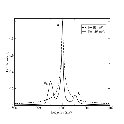
Figure 2: Spectrum (in arbitrary units) of the emission of cavity photons for $\omega_{C}=1000$, $q=0.1$, $\Delta_{1}=-\Delta_{2}=0.5$, $\gamma=0.01$, $\kappa=0.1$ and $P=0.05$ and $P=10.0$ (in dashed line) with all the magnitudes in meV. $\omega_{X}=\omega_{C}+\Delta_{1}$ and $\omega_{B}=\omega_{C}+\Delta_{2}$ label the frequencies for recombination of the exciton and biexciton respectively (see text).

Figure 2 shows the emission spectra

$$S_{J}(\omega)\propto\Re\int_{0}^{\infty}d\tau e^{i\omega\tau}G^{(1)}_{J}(t,t+\tau)$$ (12)

in the stationary limit ($t\rightarrow\infty$). Results for two different pumping rates $P=0.05meV$ and $P=10meV$ are given to show that a strong pumping introduces a strong decoherence Perea et al. (2004) masking the features of the spectrum. The low pumping result shows a strong peak at the cavity mode frequency and a couple of satellites at the exciton and biexciton transition frequencies. Despite we are giving only the spectrum of cavity photons, satellites appear as a signature of the strong coupling regime.

The pair emission efficiency ($\propto G^{(2)}$) compared with the single photon emission probability ($\propto G^{(1)}$) is usually represented by a parameter ($g$ in reference Santori et al. (2002)) which in our case of continuous pumping becomes the second order coherence function at zero delay

$$g^{(2)}_{J,J^{\prime}}(\tau=0)=G^{(2)}_{J,J^{\prime}}(0)/G^{(1)}_{J}(0)G^{(1)}_{J^{\prime}}(0).$$ (13)

Figure 3 shows $g^{(2)}_{R,R}$ and $g^{(2)}_{R,L}$ for values of $q$, $\gamma$ and $\Delta$ considered above as typical of currently available samples. Now $P$ and $\kappa$ are not fixed but vary along the two axis of the figures also in experimentally accessible regimes. The results do not show a very rich structure and, worse than that, the best efficiency for emitting pairs, i.e. the highest value of $g^{(2)}_{R,L}$ is not very high.

Since we do not get the kind of results we were looking for, we consider a second set of parameters not far from the previous ones: one needs either higher values of $q$ or lower regimes for $\kappa$, in a factor of the order of 2 to 5. Therefore, we force a little bit the parameters and consider a second case. Instead of fixing all the values in $meV$, all the rates and energies are given in units of $q$ having in mind that a possible value for this scale could be $0.2meV$ or $0.3meV$. Apart from this, we maintain the ratios $\Delta_{1}=-\Delta_{2}=\Delta=5q$ and $\gamma=0.1q$, while we must change the ratio between $\kappa$ and $q$ in order to really be in a different case. Figure 4 shows $g^{(2)}_{R,R}$ and $g^{(2)}_{R,L}$ for this new set of parameters in a range of $\kappa$ and $P$ that can be reasonably expected to be achievablenot . Apart from getting a structure richer than the one in figure 3, the main advantage is a significantly larger value of $g^{(2)}_{R,L}$. Now the emission efficiency of $RL$ pairs can be considered as satisfactory as compared to the emission of single photons.

Apart from the improvement that figure 4 represents with respect to figure 3, a general trend can be drawn for both cases. For increasing $\kappa$ and decreasing $P$, $g^{(2)}_{R,L}$ increases monotonously while $g^{(2)}_{R,R}$ tends to zero, a value only accessible in the quantum regime. In the whole range of parameters, $g^{(2)}_{R,L}$ is always greater than 1. $R$ and $L$ photons can be distinguish from each other so that, as in the case of classical fields Yamamoto and Imamoglu (1999); Loudon (1973), $G^{(2)}_{R,L}\geq G^{(1)}_{R}G^{(1)}_{L}$. On the contrary, when the two photons have the same polarization, they are indistinguishable introducing the term $-1$ in the parenthesis of Eq. (9). This reduces $G^{(2)}_{R,R}$ and produces the quantum effect of having values lower than 1 for $g^{(2)}_{R,R}$, i.e. quantum sub-Poissonian distributions for the number of photonsWalls and Milburn (1994); Loudon (1973); Yamamoto and Imamoglu (1999). The continuous pumping produces an emission of pairs different to the usual sequential two-photon cascade in which the emission of the second photon is only possible after the emission of the first photonLoudon (1973).

In order to realize the significance of our results for a continuous pumping of a QD within a cavity, one must point out that available experimental results for pulsed excitation of a QD without any cavity and collinear polarization detection ($\theta=0$)Santori et al. (2002) give $g$ and $g^{(2)}$ in the (much smaller) range between 0.01 and 0.1.

Our understanding of the results in figures 3 and 4 allows us to analyze the second aspect we mentioned in the introduction: the polarization entanglement visibility $\cal{V}$ in a experiment with different linear polarizations at the two beams produced by a non-polarizing beam splitter. In order to obtain a large visibility in Eq. (11), one needs a small value of $G_{R,R}^{(2)}$. This is precisely the quantum regime with $g_{R,R}^{(2)}<1$ occurring for low $P$ and large $\kappa$ as observed in our results for $\cal{V}$ shown in figures 5 and 6. Once again, the visibility for the second set of parameters, shown in figure 6, raises up to values closer to 1 than those corresponding to the current samples case shown in figure 5.

Let us try to understand the reason why our system seems to be less efficient than expected concerning to the emission of a photon $RL$ pair (except for the regime with low $P$ and large $\kappa$ in figure 6). The actual situation is not well described by a simple picture considering that emission of one of these $RL$ pairs is significantly improved by the double resonance condition $\Delta_{1}=-\Delta_{2}$. Figure 1 shows that, in our basis, apart from the ground state there are two types of subsets with either two or four states, for instance the lowest subset with four states contains $\mid B00\rangle$, $\mid X^{+}01\rangle$, $\mid X^{-}10\rangle$ and $\mid G11\rangle$. Inside one subset, there are not transitions contributing to the correlation functions $G^{(1)}$ and $G^{(2)}$. Therefore the processes occurring inside each subset are not as important as the simple picture would imply. On the contrary, the main physics behind photon emission is coming from transitions among different subsets as depicted in figure 1.

Finally, we must stress that we have repeated our analysis for QD’s with different characteristics, in particular for two cases: i) when the two excitons $X^{+}$ and $X^{-}$ are not degenerate and ii) when there is not perfect (but close to) double resonance $\Delta_{1}\neq-\Delta_{2}$. We have found quantitative changes, but in all the cases, the results shown here remain qualitatively valid.

One can conclude that, in spite of not being as efficient as expected for emitting $RL$ pairs of photons, the system shows a rather rich and complex behavior including both quantum and classical regimes. Our results suggest that, even though currently available samples are not in the best regime, they are close enough to expect that one can achieve a regime of efficient emission of photon pairs. In the quantum regime, a post-selection procedure would allow to perform a two beams experiment with different linear polarizations in which a large polarization entanglement visibility could be achieved.

IV Acknowledgments

We are indebted to Filippo Troiani for very helpful discussions. This work was supported in part by MCYT of Spain under contract No. MAT2002-00139, CAM under Contract No. GR/MAT/0099/2004 and European Community within the RTN COLLECT.

Figure 1: (Color on line) Ladder of levels (black continuous lines) for a four-state QD coupled to a cavity mode with the two possible ($R,L$) circular polarizations. States are labeled as described in the text with $Gn_{R}n_{L}$ ($n_{R},n_{L}=0,1,2,...$). Double (purple) continuous lines depict the coupling $q_{i,J}$, dashed (red) lines the pumping with rate $P$, dotted (blue) lines the leaky modes emission with rate $\gamma$ and dash-dotted (blue) lines the emission of cavity modes with rate $\kappa$. Pumping and emission lines in the upper part of the diagram are not plotted in order to simplify the figure.

Figure 3: (Color on line) Second order coherence functions $g^{(2)}_{R,R}$ and $g^{(2)}_{R,L}$ describing the photon pair emission efficiency ($\propto G^{(2)}$) compared with the single photon emission probability ($\propto G^{(1)}$). $q=0.1$meV, $\Delta_{1}=-\Delta_{2}=0.5$meV and $\gamma=0.01$meV. The line where $g^{(2)}_{R,R}=1$ is labeled.

Figure 4: (Color on line) Second order coherence functions $g^{(2)}_{R,R}$ and $g^{(2)}_{R,L}$ describing the photon pair emission efficiency ($\propto G^{(2)}$) compared with the single photon emission probability ($\propto G^{(1)}$). $\Delta_{1}=-\Delta_{2}=5$, $\gamma=0.1$ in units of $q$. The line where $g^{(2)}_{R,R}=1$ is labeled.

Figure 5: (Color on line) Polarization entanglement visibility $\cal{V}$ for a pair of photons with two different linear polarizations. $q=0.1$meV, $\Delta_{1}=-\Delta_{2}=0.5$meV, $\gamma=0.01$meV.

Figure 6: (Color on line) Polarization entanglement visibility $\cal{V}$ for a pair of photons with two different linear polarizations. $\Delta_{1}=-\Delta_{2}=5$, $\gamma=0.1$ in units of $q$.

References

- Gerard et al. (1998) J. Gerard, B. Sermage, B. Gayral, B. Legrand, E. Costard, and V. Thierry-Mieg, Phys. Rev. Lett. 81, 1110 (1998).
- Michler et al. (2000) P. Michler, A. Kiraz, C. Becher, W. Schoenfeld, P. Petroff, L. Zhang, E. Hu, and A. Imamoglu, Science 290, 2282 (2000).
- Moreau et al. (2001) E. Moreau, I. Robert, J. Gerard, I. Abram, L. Manin, and V. Thierry-Mieg, App. Phys. Lett. 79, 2865 (2001).
- Santori et al. (2002) C. Santori, D. Fattal, J. Vuckovic, G. Solomon, and Y. Yamamoto, Nature 419, 594 (2002).
- Pelton et al. (2002) M. Pelton, C. Santori, J. Vuckovic, B. Zhang, G. Solomon, J. Plant, and Y. Yamamoto, Phys. Rev. Lett. 89, 233602 (2002).
- Benyoucef et al. (2004) M. Benyoucef, S. Ulrich, P. Michler, J. Wiersig, F. Jahnke, and A. Forchel, New Journal of Phys. 6, 91 (2004).
- Reithmaier et al. (2004) J. Reithmaier, G. Sek, A. L ffler, C. Hofmann, S. Kuhn, S. Reitzenstein, L. Keldysh, V. Kulakovskii, T. Reinecke, and A. Forchel, Nature 432, 197 (2004).
- Yoshie et al. (2004) T. Yoshie, A. Scherer, J. Hendrickson, G. Khitrova, H. Gibbs, C. Ell, O. Shchekin, and D. Deppe, Nature 432, 200 (2004).
- Peter et al. (2004) E. Peter, P. Senellart, D. Martrou, A. Lemaitre, and J. Bloch, quant-ph/04111076 (2004).
- Walls and Milburn (1994) D. Walls and G. Milburn, in Quantum optics (Springer-Verlag, Berlin, 1994).
- Panzarini and Andreani (1999) G. Panzarini and L. Andreani, Phys. Rev. B 60, 16799 (1999).
- Yamamoto et al. (2002) Y. Yamamoto, M. Pelton, C. Santori, G. Solomon, O. Benson, J. Vuckovic, and A. Scerer, in Semiconductor spintronics and quantum, computation, edited by D.D.Awschalom, D.Loss, and N.Samarth (Springer-Verlag, New York, 2002), pp. 277–305.
- Hong et al. (1987) C. Hong, Z. Ou, and L. Mandel, Phys. Rev. Lett. 59, 2044 (1987).
- Ou and Mandel (1988) Z. Ou and L. Mandel, Phys. Rev. Lett. 61, 50 (1988).
- Kwiat et al. (1999) P. Kwiat, E. Waks, A. White, I. Appelbaum, and P. Eberhard, Phys. Rev. A 60, R773 (1999).
- Volz et al. (2001) J. Volz, C. Kurtsiefer, and H. Weinfurter, App. Phys. Lett. 79, 869 (2001).
- Zwiller et al. (2002) V. Zwiller, P. Jonsson, H. Blom, S. Jeppesen, M. Pistol, L. Samuelson, A. Katznelson, E. Kotelnikov, V. Evtikhiev, and G. Borjk, Phys. Rev. B 66, 53814 (2002).
- Bonadeo et al. (1998) N. Bonadeo, J. Erland, D. Gammon, D. Park, D. Katzer, and D. Steel, Science 282, 1473 (1998).
- Kulakovskii et al. (1999) V. Kulakovskii, G. Bacher, R. Weigand, T. Kummell, A. Forchel, E. Borovitskaya, K. Leonardi, and D. Hommel, Phys. Rev. Lett. 82, 1780 (1999).
- Bayer et al. (2002) M. Bayer, G. Ortner, O. Stern, A. Kuther, A. Gorbunov, A. Forchel, P. Hawrylak, S. Fafard, K. Hinzer, T. Reinecke, et al., Phys. Rev. B 65, 195315 (2002).
- Stace et al. (2003) T. Stace, G. Milburn, and C. Barnes, Phys. Rev. B 67, 085317 (2003).
- Benson and Yamamoto (1999) O. Benson and Y. Yamamoto, Phys. Rev. A 59, 4756 (1999).
- Perea et al. (2004) J. I. Perea, D. Porras, and C. Tejedor, Phys. Rev. B 70, 115304 (2004).
- Cohen-Tannoudji et al. (1992) C. Cohen-Tannoudji, J. Dupont-Roc, and G. Grynberg, in Atom-photon interactions (Wiley-Interscience, New Yrok, 1992).
- Scully and Zubairy (1997) M. Scully and M. Zubairy, in Quantum optics (Cambridge University Press, Cambridge, 1997).
- (26) If one takes meV as in figure 3, the range of parameters of figure 4 is below and to the left of the range of figure 3.
- Yamamoto and Imamoglu (1999) Y. Yamamoto and A. Imamoglu, in Mesoscopic quantum optics (Wiley, New York, 1999).
- Loudon (1973) R. Loudon, in The quantum theory of light (Oxford, Oxford, 1973).