On Modelling adiabatic $N$-soliton interactions in external potentials

Abstract

We analyze perturbed version of the complex Toda chain (CTC) in an attempt to describe the adiabatic $N$-soliton train interactions of the perturbed nonlinear Schrödinger equation (NLS). We study perturbations with weak quadratic and periodic external potentials by both analytical and numerical means. The perturbed CTC adequately models the $N$-soliton train dynamics for both types of potentials. As an application of the developed theory we consider the dynamics of a train of matter - wave solitons confined in a parabolic trap and optical lattice, as well as tilted periodic potentials.

1 Introduction

The $N$-soliton train interactions for the nonlinear Schrödinger equation (NLS) and its perturbed versions

$$iu_{t}+{1\over 2}u_{xx}+|u|^{2}u(x,t)=i\epsilon R[u],$$ (1)

started with the pioneering paper [1], by now has been extensively studied (see [2, 3, 4, 5, 6] and references therein). Several other nonlinear evolution equations (NLEE) were also studied, among them the modified NLS equation [8, 9, 10, 11, 12], some higher NLS equations [6], the Ablowitz-Ladik system [7] and others.

Below we concentrate on the perturbed NLS eq. (1). By $N$-soliton train we mean a solution of the (perturbed) NLS fixed up by the initial condition:

$$u(x,t=0) = \sum_{k=1}^{N}u_{k}^{\rm 1s}(x,t=0),\qquad u_{k}^{\rm 1s}(x,t)={2\nu_{k}e^{i\phi_{k}}\over\cosh z_{k}},$$ (2)

$$z_{k}(x,t) = 2\nu_{k}(x-\xi_{k}(t)),\qquad\xi_{k}(t)=2\mu_{k}t+\xi_{k,0}$$ (3)

$$\phi_{k}(x,t) = {\mu_{k}\over\nu_{k}}z_{k}+\delta_{k}(t),\qquad\delta_{k}(t)=W_{k}t+\delta_{k,0},$$ (4)

Each soliton has four parameters: amplitude $\nu_{k}$, velocity $\mu_{k}$, center of mass position $\xi_{k}$ and phase $\delta_{k}$. The adiabatic approximation uses as a small parameter $\varepsilon_{0}\ll 1$ the soliton overlap which falls off exponentially with the distance between the solitons. Then the soliton parameters must satisfy [1]:

$$|\nu_{k}-\nu_{0}|\ll\nu_{0},\quad|\mu_{k}-\mu_{0}|\ll\mu_{0},\quad|\nu_{k}-\nu_{0}||\xi_{k+1,0}-\xi_{k,0}|\gg 1,$$ (5)

where $\nu_{0}={1\over N}\sum_{k=1}^{N}\nu_{k}$, and $\mu_{0}={1\over N}\sum_{k=1}^{N}\mu_{k}$ are the average amplitude and velocity respectively. In fact we have two different scales:

$$|\nu_{k}-\nu_{0}|\simeq\varepsilon_{0}^{1/2},\qquad|\mu_{k}-\mu_{0}|\simeq\varepsilon_{0}^{1/2},\qquad|\xi_{k+1,0}-\xi_{k,0}|\simeq\varepsilon_{0}^{-1}.$$

One can expect that the approximation holds only for such times $t$ for which the set of $4N$ parameters of the soliton train satisfy (5).

Equation (1) finds a number of applications to nonlinear optics and for $R[u]\equiv 0$ is integrable via the inverse scattering transform method [13, 14]. The $N$-soliton train dynamics in the adiabatic approximation is modelled by a complex generalization of the Toda chain [15]:

$$\frac{{\rm d}^{2}Q_{j}}{{\rm d}t^{2}}=16\nu_{0}^{2}\left(e^{Q_{j+1}-Q_{j}}-e^{Q_{j}-Q_{j-1}}\right),\qquad j=1,\dots,N.$$ (6)

The complex-valued $Q_{k}$ are expressed through the soliton parameters by:

$$Q_{k}(t)=2i\lambda_{0}\xi_{k}(t)+2k\ln(2\nu_{0})+i(k\pi-\delta_{k}(t)-\delta_{0}),$$ (7)

where $\delta_{0}=1/N\sum_{k=1}^{N}\delta_{k}$ and $\lambda_{0}=\mu_{0}+i\nu_{0}$. Besides we assume free-ends conditions, i.e., $e^{-Q_{0}}\equiv e^{Q_{N+1}}\equiv 0$.

Note that the $N$-soliton train is not an $N$-soliton solution. The spectral data of the corresponding Lax operator $L$ is nontrivial also on the continuous spectrum of $L$. Therefore the analytical results from the soliton theory can not be applied. Besides we want to treat solitons moving with equal velocities and also to account for the effects of possible nonintegrable perturbations $R[u]$.

The present paper extends the results of several previous ones: see Refs. [2, 3, 4, 5, 12, 16]. Recently with the realization of Bose-Einstein condensation of dilute atomic gases it became important to study NLS equation with additional potential term $iR[u]=V(x)u(x,t)$, see [17, 18]. We continue the analysis in [6] and in our more recent reports [19], of the corresponding perturbed CTC (PCTC) model for quadratic and periodic potentials $V(x)$. Our results give additional confirmation of the stabilization properties of the periodic potentials observed in [20, 21] in a different physical setup.

We also pay attention to the so-called tilted periodic potentials, which are superpositions of periodic and linear potentials. The effect of the linear potential is that it can, if it is strong enough, overcome the confining effect of the periodic potential. As a result we can have one or more of the solitons extracted out of the train. We also demonstrate that the PCTC provides an adequate description also for these types of potentials.

2 The importance of the CTC model

The fact [15, 22] that the CTC, like the (real) Toda chain (RTC), is a completely integrable Hamiltonian system allows one to analyze analytically the asymptotic behavior of the $N$-soliton trains. However unlike the RTC, the CTC has richer variety of dynamical regimes [2, 5, 23] such as:

• asymptotically free motion if $v_{j}\neq v_{k}$ for $j\neq k$; this is the only dynamical regime possible for RTC;

• $N$-s bound state if $v_{1}=\dots=v_{N}$ but $\zeta_{k}\neq\zeta_{j}$ for $k\neq j$;

• various intermediate (mixed) regimes; e.g., if $v_{1}=v_{2}>\dots>v_{N}$ but $\zeta_{k}\neq\zeta_{j}$ for $k\neq j$ then we will have a bound state of the first two solitons while all the others will be asymptotically free;

• singular and degenerate regimes if two or more of the eigenvalues of $L$ become equal, e.g., $\zeta_{1}=\zeta_{2}\dots$ and $\zeta_{j}\neq\zeta_{k}$ for $2<j\neq k$.

By $\zeta_{k}=v_{k}+iw_{k}$ above we have denoted the eigenvalues of the Lax matrix $L$ in the Lax representation $L_{\tau}=[M,L]$ of the CTC where:

$$L = \sum_{k=1}^{N}b_{k}E_{kk}+\sum_{k=1}^{N-1}a_{k}(E_{k,k+1}+E_{k+1,k}),$$ (8)

$$b_{k} \equiv -{1\over 2}{dQ_{k}\over d\tau}={1\over 2}(\mu_{k}+i\nu_{k}),\qquad a_{k}={1\over 2}\exp((Q_{k+1}-Q_{k})/2).$$

and the matrices $E_{kp}$ are defined by $(E_{kp})_{ij}=\delta_{ki}\delta_{pj}$. The eigenvalues $\zeta_{k}$ of $L$ are time independent and complex-valued along with the first components $\eta_{k}=\vec{z}_{1}^{(k)}$ of the normalized eigenvectors of $L$:

$$L\vec{z}^{(k)}=\zeta_{k}\vec{z}^{(k)},\qquad(\vec{z}^{(k)},\vec{z}^{(m)})=\delta_{km}.$$ (9)

The set of $\{\zeta_{k}=v_{k}+iw_{k},\;\eta_{k}=\sigma_{k}+i\theta_{k}\}$ may be viewed as the set of action-angle variables of the CTC.

Using the CTC model one can determine the asymptotic regime of the $N$-soliton train. Given the initial parameters $\mu_{k}(0),\nu_{k}(0),\xi_{k}(0),\delta_{k}(0)$ of the $N$-soliton train one can calculate the matrix elements $b_{k}$ and $a_{k}$ of $L$ at $t=0$. Then solving the characteristic equation on $L|_{t=0}$ one can calculate the eigenvalues $\zeta_{k}$ to determine the asymptotic regime of the $N$-soliton train [2, 5]. Another option is to impose on $\zeta_{k}$ a specific constraint, e.g. that all $\zeta_{k}$ be purely imaginary, i.e. all $v_{k}=0$. This will provide a set of algebraic conditions $L|_{t=0}$, and on the initial soliton parameters $\mu_{k}(0),\nu_{k}(0),\xi_{k}(0),\delta_{k}(0)$ which characterize the region in the soliton parameter space responsible for the $N$-soliton bound states.

3 The perturbed NLS and perturbed CTC

We will consider several specific choices $R^{(p)}[u]$ of perturbations, $p=1,2,\dots$ in (1). In the adiabatic approximation the dynamics of the soliton parameters can be determined by the system (see [1] for $N=2$ and [2, 5] for $N>2$):

$${d\lambda_{k}\over dt} = -4\nu_{0}\left(e^{Q_{k+1}-Q_{k}}-e^{Q_{k}-Q_{k-1}}\right)+M^{(p)}_{k}+iN^{(p)}_{k},$$ (10)

$${d\xi_{k}\over dt} = 2\mu_{k}+\Xi^{(p)}_{k},\qquad{d\delta_{k}\over dt}=2(\mu_{k}^{2}+\nu_{k}^{2})+X_{k}^{(p)},$$ (11)

where $\lambda_{k}=\mu_{k}+i\nu_{k}$ and $X_{k}^{(p)}=2\mu_{k}\Xi_{k}^{(p)}+D_{k}^{(p)}$. The right hand sides of Eqs. (10)–(11) are determined by $R_{k}^{(p)}[u]$ through:

$$N_{k}^{(p)} = {1\over 2}\int_{-\infty}^{\infty}{dz_{k}\over\cosh z_{k}}\,\mbox{Re}\,\left(R_{k}^{(p)}[u]e^{-i\phi_{k}}\right),$$ (12)

$$M_{k}^{(p)} = {1\over 2}\int_{-\infty}^{\infty}{dz_{k}\,\sinh z_{k}\over\cosh^{2}z_{k}}\,\mbox{Im}\,\left(R_{k}^{(p)}[u]e^{-i\phi_{k}}\right),$$ (13)

$$\Xi_{k}^{(p)} = {1\over 4\nu_{k}^{2}}\int_{-\infty}^{\infty}{dz_{k}\,z_{k}\over\cosh z_{k}}\,\mbox{Re}\,\left(R_{k}^{(p)}[u]e^{-i\phi_{k}}\right),$$ (14)

$$D_{k}^{(p)} = {1\over 2\nu_{k}}\int_{-\infty}^{\infty}{dz_{k}\,(1-z_{k}\tanh z_{k})\over\cosh z_{k}}\mbox{Im}\,\left(R_{k}^{(p)}[u]e^{-i\phi_{k}}\right).$$ (15)

Inserting (10), (11) into (7) we derive:

$${dQ_{k}\over dt} = -4\nu_{0}\lambda_{k}+{2k\over\nu_{0}}\mathcal{N}_{0}^{(p)}+2i\xi_{k}\left(\mathcal{M}_{0}^{(p)}+i\mathcal{N}_{0}^{(p)}\right)$$ (16)

$$+ i\left(2\lambda_{0}\Xi_{k}^{(p)}-X_{k}^{(p)}-\mathcal{X}_{0}^{(p)}\right),$$

$$\mathcal{N}_{0}^{(p)} = {1\over N}\sum_{j=1}^{N}N_{j}^{(p)},\qquad\mathcal{M}_{0}^{(p)}={1\over N}\sum_{j=1}^{N}M_{j}^{(p)},\qquad\mathcal{X}_{0}^{(p)}={1\over N}\sum_{j=1}^{N}X_{j}^{(p)}.$$

In deriving eq. (16) we have kept terms of the order $\Delta\nu_{k}\simeq\mathcal{O}(\sqrt{\epsilon_{0}})$ and neglected terms of the order $\mathcal{O}(\epsilon_{0})$. The perturbations result in that $\nu_{0}$ and $\mu_{0}$ may become time-dependent. Indeed, from (10) we get:

$${d\mu_{0}\over dt}=\mathcal{M}_{0}^{(p)},\qquad{d\nu_{0}\over dt}=\mathcal{N}_{0}^{(p)},$$ (17)

The small parameter $\epsilon_{0}$ can be related to the initial distance $r_{0}=|\xi_{2}-\xi_{1}|_{t=0}$ between the two solitons. Assuming $\nu_{1,2}\simeq\nu_{0}$ we find:

$$\epsilon_{0}=\int_{-\infty}^{\infty}dx\left|u_{1}^{\rm 1s}(x,0)u_{2}^{\rm 1s}(x,0)\right|\simeq 8\nu_{0}r_{0}e^{-2\nu_{0}r_{0}}.$$ (18)

In particular, (18) means that $\epsilon_{0}\simeq 0.01$ for $r_{0}\simeq 8$ and $\nu_{0}=1/2$.

We assume that initially the solitons are ordered in such a way that $\xi_{k+1}-\xi_{k}\simeq r_{0}$. One can check [3, 12] that $N_{k}^{(p)}\simeq M_{k}^{(p)}\simeq\exp(-2\nu_{0}|k-p|r_{0})$. Therefore the interaction terms between the $k$-th and $k\pm 1$-st solitons will be of the order of $e^{-2\nu_{0}r_{0}}$; the interactions between $k$-th and $k\pm 2$-nd soliton will of the order of $e^{-4\nu_{0}r_{0}}\ll e^{-2\nu_{0}r_{0}}$.

The terms $\Xi_{k}^{(0)}$, $X_{k}^{(0)}$ are of the order of $r_{0}^{a}\exp(-2\nu_{0}r_{0})$, where $a=0$ or $1$. However they can be neglected as compared to $\widetilde{\mu}_{k}$ and $\widetilde{\nu}_{k}$, where

$$\widetilde{\mu}_{k}=\mu_{k}-\mu_{0}\simeq\sqrt{\epsilon_{0}},\qquad\widetilde{\nu}_{k}=\nu_{k}-\nu_{0}\simeq\sqrt{\epsilon_{0}},$$ (19)

The corrections to $N_{k}^{(p)}$, …, coming from the terms linear in $u$ depend only on the parameters of the $k$-th soliton; i.e., they are ‘local’ in $k$. The nonlinear terms in $u$ present in $iR^{(p)}[u]$ produce also ‘non-local’ in $k$ terms in $N_{k}^{(p)}$, ….

3.1 Nonlinear gain and second order dispersion

Consider the NLS eq. (1) with

$$R[u]=c_{0}u+c_{2}u_{xx}+d_{0}|u|^{2}u,$$ (20)

where $c_{0}$, $c_{2}$ and $d_{0}$ are real constants, see [12]. Another important factor is the order of magnitude of the perturbation coefficients $c_{0}$, $c_{2}$ and $d_{0}$ in (20). If we take them to be of the order of $\epsilon_{0}$ we find that the $N$-soliton train evolves according to:

$$\frac{d^{2}Q_{k}}{dt^{2}}=U_{00}+16\nu_{0}^{2}\left(e^{Q_{k+1}-Q_{k}}-e^{Q_{k}-Q_{k-1}}\right),$$ (21)

where for $\mu_{0}=0$ we get $U_{00}=-{8i\nu_{0}^{2}\over 3}\left(3c_{0}+8\nu_{0}^{2}d_{0}-4c_{2}\nu_{0}^{2}\right)$. This form of perturbed CTC (21) can be solved exactly:

$$Q_{k}(t)=\frac{1}{2}U_{00}t^{2}+V_{00}t+Q^{(0)}_{k}(t),$$

where $Q^{(0)}_{k}(t)$ is a solution of the unperturbed CTC and $V_{00}$ is an arbitrary constant. In this case the effect of the perturbation will be an overall motion of the center of mass of the $N$-soliton train. The relative motion of the solitons will remain the same. For larger values of the coefficients $c_{0}$, $c_{2}$ and $d_{0}$, e.g., of the order of $\sqrt{\epsilon_{0}}$ the corresponding dynamical system is more complicated and has to be treated separately.

3.2 Quadratic and periodic potentials

Let $iR[u]=V(x)u(x,t)$. Our first choice for $V(x)$ is a quadratic one:

$$V^{(1)}(x)=V_{2}x^{2}+V_{1}x+V_{0}.$$ (22)

Skipping the details we get the results:

$$N_{k}^{\rm(1)} = 0,\qquad M_{k}^{\rm(1)}=-V_{2}\xi_{k}-{V_{1}\over 2},$$ (23a)

$$\Xi_{k}^{\rm(1)} = 0,\qquad D_{k}^{\rm(1)}=V_{2}\left({\pi^{2}\over 48\nu_{k}^{2}}-\xi_{k}^{2}\right)-V_{1}\xi_{k}-V_{0},$$ (23b)

and $X_{k}^{\rm(1)}=D_{k}^{\rm(1)}$. As a result the corresponding PCTC takes the form [6]:

$${d(\mu_{k}+i\nu_{k})\over dt}=-4\nu_{0}\left(e^{Q_{k+1}-Q_{k}}-e^{Q_{k}-Q_{k-1}}\right)-V_{2}\xi_{k}-{V_{1}\over 2},$$ (24)

$${dQ_{k}\over dt}=-4\nu_{0}(\mu_{k}+i\nu_{k})-iD_{k}^{\rm(1)}-{i\over N}\sum_{j=1}^{N}D_{j}^{\rm(1)},$$ (25)

If we now differentiate (25) and make use of (24) we get [6]:

$${d^{2}Q_{k}\over dt^{2}} = 16\nu_{0}^{2}\left(e^{Q_{k+1}-Q_{k}}-e^{Q_{k}-Q_{k-1}}\right)+4\nu_{0}\left(V_{2}\xi_{k}+{V_{1}\over 2}\right)-i{dD_{k}^{\rm(1)}\over dt}-{i\over N}\sum_{j=1}^{N}{dD_{j}^{\rm(1)}\over dt}.$$

It is reasonable to assume that $V_{2}\simeq{\cal O}(\epsilon_{0}/N)$; this ensures the possibility to have the $N$-soliton train ‘inside’ the potential. It also means that both the exponential terms and the correction terms $M_{k}^{\rm(1)}$ are of the same order of magnitude. From eqs. (24) and (25) there follows that $d\nu_{0}/dt=0$ and:

$${d\mu_{0}\over dt}=-V_{2}\xi_{0}-{V_{1}\over 2},\qquad{d\xi_{0}\over dt}=2\mu_{0},$$ (26)

where $\mu_{0}$ is the average velocity and $\xi_{0}={1\over N}\sum_{j=1}^{N}\xi_{j}$, is the center of mass of the $N$-soliton train. The system of equations (26) for $V_{2}>0$ has a simple solution

$$\mu_{0}(t)=\mu_{00}\cos(\Phi(t)),\qquad\xi_{0}(t)=\sqrt{2\over V_{2}}\mu_{00}\sin(\Phi(t))-{V_{1}\over 2V_{2}},$$ (27)

where $\Phi(t)=\sqrt{2V_{2}}t+\Phi_{0}$, and $\mu_{00}$ and $\Phi_{0}$ are constants of integration. Therefore the overall effect of such quadratic potential will be to induce a slow periodic motion of the train as a whole.

Another important choice is the periodic potential

$$V^{(2)}(x)=A\cos(\Omega x+\Omega_{0}),$$ (28)

where $A$, $\Omega$ and $\Omega_{0}$ are appropriately chosen constants. NLS equation with similar potentials appear in a natural way in the study of Bose-Einstein condensates, see [17].

For $N=2$ solitons the corresponding Karpman-Solov’ev system was derived in [21]. For $N>2$ we obtain the PCTC where the integrals for $N_{k}$, $M_{k}$, $\Xi_{k}$ and $D_{k}$ are equal to [6]:

$$N_{k}^{(2)} = 0,\qquad M_{k}^{(2)}={\pi A\Omega^{2}\over 8\nu_{k}}{1\over\sinh Z_{k}}\sin(\Omega\xi_{k}+\Omega_{0}),$$ (29)

$$\Xi_{k}^{(2)} = 0,\qquad D_{k}^{(2)}=-{\pi^{2}A\Omega^{2}\over 16\nu_{k}^{2}}{\cosh Z_{k}\over\sinh^{2}Z_{k}}\cos(\Omega\xi_{k}+\Omega_{0}),$$ (30)

where $Z_{k}=\pi\Omega/(4\nu_{k})$. These results allow one to derive the corresponding perturbed CTC models. Again we find that $d\nu_{0}/dt=0$.

4 Analysis of the perturbed CTC and comparison with numerical simulations

The dynamics of an individual soliton in a train is determined by the combined action of external potential and the influence of neighboring solitons. The interaction with neighboring solitons can be either repulsive, or attractive depending on the phase relations between them. Particularly, if their amplitudes are equal and the initial phase difference between neighboring solitons is $\pi$ (as considered below) they repel each other giving rise to expanding motion in the absence of an external field [2, 3].

The external potential counterbalances the expansion, trying to confine solitons in the minima of the potential. It is the interplay of these two factors - the interaction of solitons and the action of the external potential, which gives rise to a rich dynamics of the $N$-soliton train.

To verify the adequacy of the perturbed CTC model for the description of the $N$-soliton train dynamics in external potentials we performed comparison of predictions of corresponding perturbed CTC (PCTC) system and direct simulations of the underlying NLS equation (1). Below we present results pertaining to a matter-wave soliton train in a confining (i) parabolic trap and in (ii) a periodic potential modelling an optical lattice.

Here we present the numerical verification of the PCTC model. The perturbed NLS eq. (1) is solved by the operator splitting procedure using the fast Fourier transform [24]. In the course of time evolution we monitor the conservation of the norm and energy of the N-soliton train. The corresponding PCTC equations are solved by the Runge-Kutta scheme with the adaptive stepsize control [25].

The evolution of a $N$-soliton train in the absence of potential ($V(x)=0$) is well known, see e.g. [3, 5]. These papers propose a method to determine the asymptotic dynamical regime of the CTC for a given set of initial parameters $\nu_{k}(0)$, $\mu_{k}(0)$, $\xi_{k}(0)$ and $\delta_{k}(0)$. Below we will use mainly the following set of parameters:

$$\nu_{k}(0)=1/2,\qquad\mu_{k}(0)=0,\qquad\xi_{k+1}(0)-\xi_{k}(0)=r_{0},\qquad\delta_{k}(0)=k\pi,$$ (31)

$$\nu_{k}(0)=1/2,\qquad\mu_{k}(0)=0,\qquad\xi_{k+1}(0)-\xi_{k}(0)=r_{0},\qquad\delta_{k}(0)=0.$$ (32)

These two types of initial conditions (IC) are most widely used in numeric simulations.

In the absence of potential the IC (31) ensure the so called free asymptotic regime, i.e. each soliton develops its own velocity and the distance between the neighboring solitons increases linearly in time. At the same time the center of mass of the soliton train stays at rest (see the left panel of Fig. 1). Under the IC (32) the solitons attract each other going into collisions whenever the distance between them is not large enough.

From mathematical point of view the IC (31) reduce the CTC into a standard (real) Toda chain for which the free asymptotic regime is the only possible asymptotical regime. On the contrary the IC (32) lead to singular solutions for the CTC (see [2, 5, 23]). The singularities of the exact solutions for the CTC coincide with the positions of the collisions.

Below we will study the effects of the potentials for both types of IC. One may expect that the quadratic potential will prevent free asymptotic regime of IC (31) no matter how small $V_{2}>0$ is and would not be able to prevent collisions in the case of IC (32). The periodic potential, if strong enough should be able to stabilize and bring to bound states both types of IC.

4.1 Quadratic potential

For the quadratic external potential $V(x)=V_{2}x^{2}+V_{1}x+V_{0}$ the perturbed CTC equations in terms of soliton parameters have the form:

$${d\mu_{k}\over dt} = 16\nu_{0}^{3}\left(e^{-2\nu_{0}(\xi_{k+1}-\xi_{k})}\cos\left(2\mu_{0}(\xi_{k+1}-\xi_{k})+\delta_{k}-\delta_{k+1}\right)\right.$$

$$- \left.e^{-2\nu_{0}(\xi_{k}-\xi_{k-1})}\cos\left(2\mu_{0}(\xi_{k}-\xi_{k-1})+\delta_{k-1}-\delta_{k}\right)\right)-V_{2}\xi_{k}-{V_{1}\over 2},$$

$${d\nu_{k}\over dt} = 16\nu_{0}^{3}\left(e^{-2\nu_{0}(\xi_{k+1}-\xi_{k})}\sin\left(2\mu_{0}(\xi_{k+1}-\xi_{k})+\delta_{k}-\delta_{k+1}\right)\right.$$

$$- \left.e^{-2\nu_{0}(\xi_{k}-\xi_{k-1})}\sin\left(2\mu_{0}(\xi_{k}-\xi_{k-1})+\delta_{k-1}-\delta_{k}\right)\right),$$

$${d\xi_{k}\over dt} = 2\mu_{k},$$ (35)

$${d\delta_{k}\over dt} = 2(\mu_{k}^{2}+\nu_{k}^{2})+V_{2}\left({\pi^{2}\over 48\nu_{k}^{2}}-\xi_{k}^{2}\right)-V_{1}\xi_{k}-V_{0}.$$ (36)

where $\mu_{k}$, $\nu_{k}$, $\xi_{k}$ and $\delta_{k}$ for $k=1,\dots,N$ are the $4N$ soliton parameters, see eqs. (2)-(3).

The effect of the quadratic potential on the $N$-soliton train with parameters (31) is to balance the repulsive interaction between the solitons, so that they remain bounded by the potential, as illustrated in figures: the right panel of 1 and in 2. The quadratic potentials are supposed to be weak, i.e. we choose $V_{2}$ so that

$$V_{2}\xi_{N}^{2}(0)\leq\nu_{0},\qquad V_{2}\xi_{1}^{2}(0)\leq\nu_{0}.$$ (37)

Figure 1: Left panel: $9$-soliton train with initial parameters as in eq. (31) with $r_{0}=8$ in the absence of a potential goes into free asymptotic regime. Solid lines: direct numerical simulation of the NLS equation (1); dashed lines: $\xi_{k}(t)$ as predicted by the CTC equations (4.1)-(36) with $V_{0}=V_{1}=V_{2}=0$ and $r_{0}=8$. Right panel: Evolution of a $9$-soliton train with the same initial parameters in the quadratic potential $V(x)=V_{2}x^{2}$ with $V_{2}=0.00005$. Solid lines: direct numerical simulation of the NLS equation (1); dashed lines: solution of the PCTC equations (4.1)-(36). Initially the train is placed symmetrically relative to the minimum of the potential at $x=0$.

  

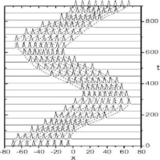
Figure 2: Harmonic oscillations of a N-soliton train initially shifted relative to the minimum of the quadratic potential $V(x)=V_{2}x^{2}$. Left panel: 9-soliton train, $V_{2}=0.00005$. Right panel: 3-soliton train, $V_{2}=0.001$. The IC of the both trains is given by (31) with $r_{0}=8$. In both panels solid lines correspond to direct simulations of the NLS equation (1), and dashed lines to numerical solution of the PCTC equations (4.1) - (36).

Figures 1 and 2 show good agreement between the PCTC model and the numerical solution of the perturbed NLS equation (1). They also show two types of effects of the quadratic potential on the motion of the $N$-soliton train: (i) the train performs contracting and expanding oscillations if its center of mass coincides with the minimum of the potential, (ii) the train oscillates around the minimum of the potential as a whole if its center of mass is shifted. In the last case contracting and expanding motions of the soliton train is superimposed to the center of mass dynamics. As one can see from the figures the period of this motion matches very well the one predicted by formula (27). Indeed, from eq. (27) it follows that the period period of the center of mass motion is $T=2\pi/\sqrt{2V_{2}}$. For the parameters in fig. 2 we have $T\simeq 628$ (for 9-soliton train), $T\simeq 140$ (for $3$-soliton train). Similar is the dynamics also for the $7$-soliton train on Fig. 3; for the parameters choosen there we have $T=314.2$, in good agreement with the numerical simulations.

Figure 3: Dynamics of a 7-soliton train placed asymmetrically relative to the minimum of the trap $V(x)=0.0002x^{2}$. Solid lines: results of direct numerical simulations of the NLS equation (1). Dashed lines: result of solution of the PCTC system (4.1) - (36) for the center of mass $\xi_{i}$. The parameters of solitons are the same as in (31) with $r_{0}=8$. The initial shift of the soliton train relative to the minimum of the parabolic trap is $10\pi$.

The direct simulations of the NLS equation (1) shows that stronger parabolic trap may cause merging of individual solitons at times of contraction, and restoring of the original configuration when the train is expanded. This behavior reminds the phenomenon of ”missing solitons” observed in the experiment [26]. However, this situation is beyond the validity of the PCTC approach.

4.2 Periodic potential

Another external potential in which the $N$-soliton train exhibits interesting dynamics is the periodic potential of the form $V(x)=A\cos(\Omega x+\Omega_{0})$. This case also may have a direct relevance to matter - wave soliton trains confined to optical lattices. The PCTC system in terms of soliton parameters has the form:

$${d\mu_{k}\over dt} = 16\nu_{0}^{3}\left(e^{-2\nu_{0}(\xi_{k+1}-\xi_{k})}\cos\left(2\mu_{0}(\xi_{k+1}-\xi_{k})+\delta_{k}-\delta_{k+1}\right)\right.$$ (38)

$$- \left.e^{-2\nu_{0}(\xi_{k}-\xi_{k-1})}\cos\left(2\mu_{0}(\xi_{k}-\xi_{k-1})+\delta_{k-1}-\delta_{k}\right)\right)+M_{k}^{(2)}(\nu_{k}),$$

$${d\nu_{k}\over dt} = 16\nu_{0}^{3}\left(e^{-2\nu_{0}(\xi_{k+1}-\xi_{k})}\sin\left(2\mu_{0}(\xi_{k+1}-\xi_{k})+\delta_{k}-\delta_{k+1}\right)\right.$$

$$- \left.e^{-2\nu_{0}(\xi_{k}-\xi_{k-1})}\sin\left(2\mu_{0}(\xi_{k}-\xi_{k-1})+\delta_{k-1}-\delta_{k}\right)\right),$$

$${d\xi_{k}\over dt} = 2\mu_{k},$$ (40)

$${d\delta_{k}\over dt} = 2(\mu_{k}^{2}+\nu_{k}^{2})+D_{k}^{(2)}(\nu_{k}),$$ (41)

where $M_{k}^{(2)}(\nu_{k})$ and $D_{k}^{(2)}(\nu_{k})$ are given in (29) and (30).

Each soliton of the train experience confining force of the periodic potential and repulsive force of neighboring solitons. Therefore, equilibrium positions of solitons do not coincide with the minima of the periodic potential. Solitons placed initially at minima of the periodic potential (Fig. 4) perform small amplitude oscillations around these minima, provided that the strength of the potential is big enough to keep solitons confined. As opposed, the weak periodic potential is unable to confine solitons, and repulsive forces between neighboring solitons (at phase difference $\pi$) induces unbounded expansion of the train.

Figure 4: Solitons (continuous line) remain confined around the minima of the periodic potential $V(x)=A\cos(x)$ (dashed line) performing small amplitude oscillations if its strength is big enough $A=0.1$.

In the intermediate region, when the confining force of the periodic potential is comparable with the repulsive forces of neighboring solitons, interesting dynamics can be observed such as the expulsion of bordering solitons from the train, as shown in the left panel of Fig. 5.

  

Figure 5: Left panel: The expulsion of solitons from the train, as obtained from direct simulations of the NLS equation (1) (solid lines), and as predicted by PCTC system (38)-(41) for the center of mass $\xi_{i}$ (dashed lines). The IC of the $7$-soliton train are given by (31) with $r_{0}=8$; the parameters of the periodic potential $V(x)=A\cos(\Omega x+\Omega_{0})$ are $A=0.001,\ \Omega=\pi/4,\ \Omega_{0}=0$. Right panel: Oscillations of the 5-soliton train with IC given by (31) with $r_{0}=9$; in a moderately weak periodic potential, $A=0.0005$, $\Omega=2\pi/9$, $\Omega_{0}=0$. Solid and dashed lines correspond, respectively, to numerical solution of the NLS eq. (1) and PCTC system (38) - (41).

This phenomenon, revealing the complexity of the internal dynamics of the train, can be explained as follows. Each soliton performs nonlinear oscillations within individual potential wells under repulsive forces from neighboring solitons. When the amplitude of oscillations of particular solitons grow and two solitons closely approach each other, a strong recoil momentum can cause the soliton to leave the train, overcoming barriers of the periodic potential. In Fig. 5 this happens with bordering solitons (the other solitons remain bounded under long time evolution). It is noteworthy to stress that this phenomenon is well described by the PCTC model, as is evident from Fig. 5, left panel.

On the right panel of the same figure we have similar IC as in (31) and we have choosen again the initial positions of the solitons to coincide with the minima of the periodic potential $V(x)=A\cos(\Omega x+\Omega_{0})$; i.e. $r_{0}=2\pi/\Omega$. The values of $A=0.0005$ and $r_{0}=9$ in the right panel of Fig. 5 now are such that the solitons form a bound state. Therefore for any given initial distance $r_{0}$ there is a critical value $A_{\rm cr}(r_{0})$ for $A$ such that for $A>A_{\rm cr}(r_{0})$ the soliton train with IC (31) will form a bound state.

In contrast to the quadratic potentials, the weak periodic potential is unable to confine solitons, and repulsive forces between neighboring solitons (at $\nu_{k}(0)=1/2,\ \delta_{k}(0)=k\pi$) induces unbounded expansion of the train similar to what was shown in the left panel of Fig. 1.

The periodic potential can play stabilizing role also for the IC (32), when the zero phase difference between neighboring solitons correspond to their mutual attraction. If the periodic potential is strong enough, solitons do not experience collision. The weak periodic potential cannot prevent solitons from collisions, which eventually leads to destruction of the soliton train, as illustrated in Fig. 6. Again for any given initial distance $r_{0}$ there will be a critical value $A_{\rm cr}^{\prime}(r_{0})$ for $A$ such that for $A>A^{\prime}_{\rm cr}(r_{0})$ the soliton train with IC (32) will form a bound state avoiding collisions.

  

Figure 6: Dynamics of a 5-soliton train with zero phase difference between neighboring solitons, in the periodic potential $V(x)=A\cos(\Omega x+\Omega_{0})$ with $\Omega=\pi/4$, $\Omega_{0}=0$, and $r_{0}=8$. Left panel: When the periodic potential is strong enough $A=0.02$, the N-soliton train remain confined, each soliton performing small amplitude oscillations around the minima of individual cells. Right panel: Weaker periodic potential $A=0.01$ cannot prevent solitons from collisions, which destroy the train. Solid and dashed lines correspond, respectively, to numerical solution of the NLS eq. (1) and PCTC system (38) - (41).

4.3 Tilted periodic potential

Now we consider the dynamics of a N - soliton train in a tilted periodic potential, which is the combination of periodic and linear potentials

$$V(x)=A\cos(\Omega x+\Omega_{0})+Bx.$$ (42)

This potential is of particular interest in studies of Bose-Einstein condensates. A train of repulsive BEC loaded in such a potential (where the periodic potential was a 1D optical lattice and the linear one was due to the gravitation) exhibited Bloch oscillations [27]. At each period of these oscillations condensate atoms residing in individual optical lattice cells coherently tunneled through the potential barriers. This was the first experimental demonstration of a pulsed atomic laser [27]. Recently a new model of a pulsed atomic laser was theoretically developed in [28], where the solitons of attractive BEC were considered as carriers of coherent atomic pulses.

Controlled manipulation with matter - wave solitons is important issue in these applications. Below we demonstrate that solitons of attractive BEC confined in tilted optical lattice can be flexibly manipulated by adjustment of the strength of the linear potential. In Fig. 7 we show the extraction of different number of solitons from the 5-soliton train by increasing the strength of the linear potential $B$, as obtained from direct simulations of the NLS equation (1) and numerical integration of the PCTC system (38) - (41) with

$$M_{k}^{(2)} = {\pi A\Omega^{2}\over 8\nu_{k}}{1\over\sinh Z_{k}}\sin(\Omega\xi_{k}+\Omega_{0})-\frac{1}{2}B,$$ (43)

$$D_{k}^{(2)} = -{\pi^{2}A\Omega^{2}\over 16\nu_{k}^{2}}{\cosh Z_{k}\over\sinh^{2}Z_{k}}\cos(\Omega\xi_{k}+\Omega_{0})-B\xi_{k}.$$ (44)

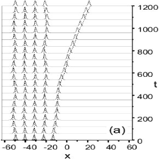
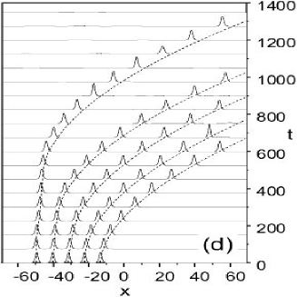
Figure 7: Controlled withdrawal of solitons from the 5-soliton train by adjusting the strength of the linear potential (42) with parameters: $A=0.0005$, $\Omega=2\pi/9$, $\Omega_{0}=0$. Depending on the tilt, different number of solitons can be pulled out of the train: (a) one soliton at $B=-0.00003$, (b) two at $B=-0.00011$, (c) four at $B=-0.0002$ and (d) five at $B=-0.0003$. The initial phase difference and separation between neighboring solitons in the train are, respectively, $\pi$ and $9$. Initially the train is shifted by $-10\pi$ with respect to $x=0$ for graphical convenience. Solid and dashed lines correspond, respectively, to direct simulations of the NLS equation (1) and numerical integration of the PCTC system (38) - (41) .

As is evident from Fig. 7, the PCTC model provides adequate description of the dynamics of a N-soliton train in a tilted periodic potential. A small divergence between predictions for the trajectory of the left border soliton in Fig. 7 (d), is due to the imperfect absorption of solitons from the right end of the integration domain. Reflected waves enter the integration domain and interact with solitons, which causes the discrepancy.

5 Conclusions

We have studied the dynamics of the $N$-soliton train confined to external fields (quadratic and periodic potentials). Both the analytical treatment in the framework of the PCTC model, and numerical analysis by direct simulations of the underlying NLS equation show that the PCTC is adequate for description of the $N$-soliton interactions in external potentials. Relevance of this study to the research on matter-wave soliton trains in magnetic traps and optical lattices is briefly mentioned.

Like any other model, the predictions of the CTC should be compared with the numerical solutions of the corresponding NLEE. Such comparison between the CTC and the NLS has been done thoroughly in [2, 3, 5] and excellent match has been found for all dynamical regimes. This means that the CTC may be viewed as an universal model for the adiabatic $N$-soliton interactions for several types of NLS.

For the perturbed CTC equations such comparison has been just started; the good agreement shown in the figures above supports the hope that the region of applicability of PCTC can be widened.

More detailed investigation of the $N$-soliton train interactions under different types of external potentials and for diffetent types of initial soliton parameters will be published in subsequent papers.

References

• [1] V. I. Karpman, V. V. Solov’ev, Physica D 3D, 487-502, (1981).
• [2] V. S. Gerdjikov, D. J. Kaup, I. M. Uzunov, E. G. Evstatiev, Phys. Rev. Lett. 77, 3943-3946 (1996).
• [3] V. S. Gerdjikov, I. M. Uzunov, E. G. Evstatiev, G. L. Diankov, Phys. Rev. E 55, No 5, 6039-6060 (1997).
• [4] J. M. Arnold, JOSA A 15, 1450-1458 (1998); Phys. Rev. E 60, 979-986 (1999).
• [5] V. S. Gerdjikov, E. G. Evstatiev, D. J. Kaup, G. L. Diankov, I. M. Uzunov, Phys. Lett. A 241, 323-328 (1998).
• [6] V. S. Gerdjikov, On Modelling Adiabatic $N$-soliton Interactions. Effects of perturbations. In ”Nonlinear Waves: Classical and Quantum Aspects”, Eds.: F. Kh. Abdullaev and V. Konotop. (Kluwer, 2004), 15 - 28.
• [7] E. V. Doktorov, N. P. Matsuka, V. M. Rothos. Phys. Rev. E 69, 056607 (2004).
• [8] Y. Kodama, A. Hasegawa, IEEE J. of Quant. Electron. QE-23, 510 - 524 (1987).
• [9] V. S. Gerdjikov, M. I. Ivanov, P. P. Kulish, Theor. Math. Phys. 44, No.3, 342–357, (1980), (In Russian). V. S. Gerdjikov, M. I. Ivanov, Bulgarian J. Phys. 10, No.1, 13–26; No.2, 130–143, (1983), (In Russian).
• [10] V. S. Shchesnovich and E. V. Doktorov, Physica D 129, 115 (1999); E. V. Doktorov and V. S. Shchesnovich, J. Math. Phys. 36, 7009 (1995).
• [11] V. S. Gerdjikov, E. V. Doktorov, J. Yang, Phys. Rev. E 64, 056617 (2001).
• [12] V. S. Gerdjikov, I. M. Uzunov, Physica D 152-153, 355-362 (2001).
• [13] V. E. Zakharov, S. V. Manakov, S. P. Novikov, L. P. Pitaevskii, Theory of solitons: the inverse scattering method. (Plenum, N.Y.: Consultants Bureau, 1984).
• [14] L. A. Takhtadjan and L. D.  Fadeev, Hamiltonian Approach to Soliton Theory  (Springer Verlag, Berlin, 1986).
• [15] S. V. Manakov, JETPh 67, 543 (1974); H. Flaschka. Phys. Rev. B9, 1924–1925, (1974);
• [16] V. S. Gerdjikov, Complex Toda Chain – an Integrable Universal Model for Adiabatic $N$-soliton Interactions. In Proc. of the Workshop ”Nonlinear Physics: Theory and Experiment. II”, Gallipoli, June-July 2002; Eds.: M. Ablowitz, M. Boiti, F. Pempinelli, B. Prinari. p. 64-70 (2003).
• [17] J. C. Bronski, L. D. Carr, B. Deconinck, J. N. Kutz, Phys. Rev. E 63, 036612 (2001); Phys. Rev. Lett. 86, 1402–1405 (2001); J. C. Bronski, L. D. Carr, R. Carretero-Gonzales, B. Deconinck, J. N. Kutz, K. Promislow, Phys. Rev. E 64, 056615 (2001); F. Kh. Abdullaev, B. B. Baizakov, S. A. Darmanyan, V. V. Konotop, M. Salerno, Phys. Rev. A 64, 043606 (2001).
• [18] R. Carretero-Gonzalez and K. Promislow, Phys. Rev. A 66, 033610 (2002).
• [19] V. S. Gerdjikov, B. B. Baizakov, M. Salerno, Modelling adiabatic N-soliton interactions and perturbations. In: Proceedings of the workshop ”Nonlinear Physics: Theory and Experiment. III”, Gallipoli, 2004;
Eds.: M. Ablowitz, M. Boiti, F. Pempinelli, B. Prinari (In press).
V. S. Gerdjikov, B. B. Baizakov, On Modelling Adiabatic $N$-soliton Interactions and Perturbations. Effects of external potentials. Report at the International Conference ”Gravity, astrophysics and strings at the Black sea”, Kiten, Bulgaria, June 10 - 16 (2004).
• [20] S. Wabnitz. Electron. Lett. 29, 1711 (1993);
• [21] I. M. Uzunov, M. Gölles, F. Lederer, JOSA B 12, No. 6, 1164 (1995);
I. M. Uzunov, M. Gölles, F. Lederer, Phys. Rev. E 52, 1059-1071 (1995).
• [22] J. Moser, In Dynamical Systems, Theory and Applications. Lecture Notes in Physics, v. 38, Springer Verlag, (1975), p. 467.
• [23] V. S. Gerdjikov, E. G. Evstatiev, R. I. Ivanov, The complex Toda chains and the simple Lie algebras – solutions and large time asymptotics, J. Phys. A: Math & Gen. 31, 8221-8232 (1998).
• [24] T. R. Taha and M. J. Ablowitz, J. Comp. Phys. 55, 203 (1984).
• [25] W. H. Press, S. A. Teukolsky, W. T. Vetterling, and B. P. Flannery, Numerical Recipes. The Art of Scientific Computing. (Cambridge University Press, 1996).
• [26] K. E. Strecker, G. B. Partridge, A. G. Truscott, and R. G. Hulett, Nature, 417, 150 (2002).
• [27] B. P. Anderson, M. A. Kasevich, Science, 282, 1686 (1998).
• [28] L. D. Carr and J. Brand, Phys. Rev. A 70, 033607 (2004).