[

Thermopower in superconductors

Abstract

The thermopower of superconductors measured via the magnetic flux in bimetallic loop is evaluated. It is shown that by a standard matching of the electrostatic potential, known as the Bernoulli potential, one explains the experimentally observed amplitude and the divergence in the vicinity of the critical temperature.

]

The thermopower is a widely used tool to study electronic properties of conductive materials. An exception are superconductors, where the supercurrent cancels any diffusive current so that the zero net current or voltage are observed. This feature is known from 1935 [1] and since then there were a number of attempts to access diffusive currents in an indirect way.

Already in 1944 Ginzburg [2] noticed that in inhomogeneous systems like bimetallic loops, the counter-flowing supercurrent creates a magnetic flux. The boom in this field came thirty years later. In 1974 Garland and Van Harlingen proposed a simple phenomenological theory [3] and Gal’perin, Gurevich and Kozub published a microscopic treatment [4] based on the Boltzmann-type approach. These theories predicted fluxes of similar amplitudes and temperature dependences.

In the same year Zavaritskii presented first experimental data [5] and he was soon followed by others [6, 7, 8]. Experimental results were a surprise. Zavaritskii [5] and Falco [7] observed the expected temperature dependence, but Pegrum, Guénault and Pickett [6] and Van Harlingen and Garland [8] monitored a thermally induced magnetic flux by five orders of magnitude larger. Moreover, the theory predicts that close to $T_{c}$ the flux $\Phi$ diverges as ${d\Phi\over dT}\propto(T_{\rm c}-T)^{-1}$, while a steeper divergence ${d\Phi\over dT}\propto(T_{\rm c}-T)^{-3/2}$ was observed [6, 8]. The experimental situation in the late 1970 is reviewed in Ref. [9].

The giant flux stimulated a number of theoretical studies [10, 11, 12, 13, 14, 15] that explored various additional components ranging from a trapped flux, over impurities, over interfaces, to an influence of supercurrent flow. Most of these ingredients bring only a minor correction to the original prediction. It was speculated, that the only sizable contribution can come from the trapped flux, which increasingly leaks into the ring as the temperature approaches its critical value. All these speculations were terminated by measurements of Van Harlingen, Heidel and Garland [16]. To avoid the penetration of the external magnetic field they used the toroidal geometry and convincingly demonstrated that the large magnetic flux with the ${d\Phi\over dT}\propto(T_{\rm c}-T)^{-3/2}$ divergence is a genuine effect. By comparing a number of samples they could conclude that the flux is proportional to the thermopower in the normal state and therefore that it is indeed caused by the thermal diffusion of electrons.

The lack of at least a qualitative theory has discouraged further measurements in this direction and the thermopower joined the family of puzzling transport properties in superconductors. Alternative measurements of the thermopower via the superconducting fountain effect [17] or the charge imbalance in the conversion region [18] yield theoretically expected values but they have a rather low accuracy. In result, the values of the thermoelectric coefficients of superconductors are still not available, what contrasts with extensive data gathered for superconducting materials above $T_{\rm c}$.

New theoretical interest in the giant magnetic flux emerged after seventeen years. Marinescu and Overhauser [19] have analyzed the theory of Gal’perin, Gurevich and Kozub [4] and concluded, that its failure indicates a conceptual mistake in the underlying Boltzmann type transport theory developed by Bardeen, Rickayzen and Tewordt [20]. They made an ad hoc modification of the transport theory by including the momentum exchange between the condensate and quasiparticles. With this modification, a good agreement between theory and experimental data was reached.

The modified transport theory, however, is in conflict with other properties of superconductors as discussed recently by Gal’perin, Gurevich, Kozub and Shelankov [21]. From the time-reversal symmetry they showed that this theory predicts dissipative currents also in equilibrium systems with inhomogeneous chemical composition, i.e., in any real superconductor.

Here we show that explanation of the thermopower does not require any changes in the theory of transport in superconductors. The legitimate request of Marinescu and Overhauser to cover properly the balance of forces between the superconducting and normal electrons is naturally covered by the theory of electrostatic potential in superconductors known as the Bernoulli potential. Unlike forces ad hoc added to the kinetic equation, forces derived from a scalar potential cannot result in an artificial dissipation.

Below we demonstrate that the giant magnetic flux can be described in a simple manner with the help of the Bernoulli potential. Our approach parallels the textbook theory of thermopower in normal metals in that we evaluate the net current in the sample from the requirement of the electrostatic potential matching.

We will use notation related to the experimental setup of Van Harlingen, Heidel and Garland [16] shown in Fig. 1. The sample is a toroid with the internal cylinder from the Lead and the external one from the Indium. The magnetic flux $\Phi$ in question is restricted to the volume between cylinders, i.e., it is inside the toroidal cavity. The diamagnetic current $J$ corresponding to the flux $\Phi$ flows on the outer surface of Lead and the inner surface of Indium. The flux is linear in the current,

$$\Phi=J{1\over 2\pi}\mu_{0}D\ln{r_{\rm In}\over r_{\rm Pb}},$$ (1)

where $D$ is the length of the sample, and $r_{\rm In,Pb}$ are the radii which enclose the flux.

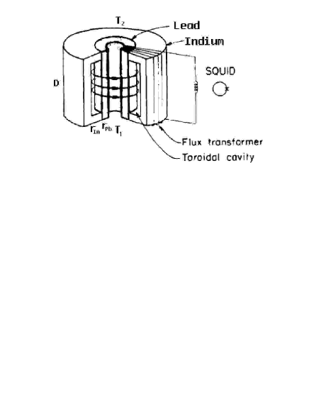
FIG. 1.: The toroidal sample of Van Harlingen at al [16]. The measured flux $\Phi$ is in the toroidal cavity.

The experiment is aimed to measure the transport coefficient $L_{T}$ which determines the diffusive electric current ${\bf j}_{\rm dif}=-L_{T}\nabla T$ caused by the temperature gradient $\nabla T$. As already mentioned, ${\bf j}_{\rm dif}$ is not observable since it is cancelled by the supercurrent ${\bf j}=-{\bf j}_{\rm dif}$. The theory of Garland and Van Harlingen [3] uses the London gauge to find the vector potential ${\bf A}=-\mu_{0}\lambda^{2}{\bf j}$, where $\lambda$ is the London penetration depth. The flux is then an integral along the bimetallic loop, $\Phi_{\rm G}=\oint d{\bf rA}=-\mu_{0}\oint d{\bf r}\lambda^{2}L_{T}\nabla T$.

The London gauge is justified only for small fluxes. The data from [16] show, however, that the flux is large so that it is of form $\Phi=N\Phi_{0}+\Phi_{\rm G}$, where $N$ is an integer quantum number of the superconducting condensate and $\Phi_{0}$ is the elementary flux. Estimates [16] indicate that $\Phi_{\rm G}\ll\Phi_{0}$, therefore to understand the giant flux, we have to find which state $N$ is the most favorable for the system with the imposed temperature gradient. Measured values of $N$ in [16] range up to 250. These values are sufficiently large for the classical approximation, where $N$ is treated as a continuous variable. Accordingly, we will not assume quantum restrictions of the flux $\Phi$.

The mechanism by which the flux arises is as follows. The diffusive current generates magnetic field, which is screened by the counterflowing supercurrent. In the surface layer of the London penetration depth thickness, the cancellation is not complete. Accordingly, the supercurrent density is a sum of the counter-flow $-{\bf j}_{\rm dif}$ and a missing counter-flow $j{\rm e}^{-x/\lambda}$, where $x$ is a distance from the surface enclosing the cavity. We call it a diamagnetic current, as it screens the bulk of superconductor from the magnetic field, which is present in the toroidal cavity.

Our aim is to find amplitudes $j$ in the Indium and the Lead. The total current $J=\int d^{2}{\bf r}({\bf j}+{\bf j}_{\rm dif})$ is the integral of the current density across each cylinder, i.e., $J=2\pi r_{\rm In}\lambda_{\rm In}j_{\rm In}$, and due to continuity condition also $J=-2\pi r_{\rm Pb}\lambda_{\rm Pb}j_{\rm Pb}$. Since $\lambda$ depends on the temperature, the surface values of the diamagnetic current densities $j_{\rm In,Pb}$ change along the temperature gradient, while the product $\lambda j$ stays constant.

Now we specify the condition for the total current $J$ from the requirement of the scalar potential matching. As was observed by Bok and Klein [23] and with a higher precision by Morris and Brown [24, 25], current in the superconductor induces perpendicular electric field. It is well approximated by the electrostatic potential of Bernoulli type [22]

$$\varphi={n_{s}\over n}{1\over 2}mv^{2},$$ (2)

where $n_{s}$ is the density of superconducting electrons. The velocity of the superconducting electrons at the surface is given by the current density,

$$v={{\bf j}\over en_{s}}={L_{T}\nabla T\over en_{s}}\pm{J\over 2\pi r\lambda en_{s}},$$ (3)

where plus applies for the Indium and minus for the Lead, in which the total current flows in opposite direction. The first term is due to the compensating supercurrent $-{\bf j}_{\rm diff}$, the second term is caused by the diamagnetic current $j$.

The electrostatic potential has to be continuous, therefore the potential differences created by the temperature gradient in the Lead and the Indium has to be equal,

$$\varphi_{\rm Pb}(T_{2})-\varphi_{\rm Pb}(T_{1})=\varphi_{\rm In}(T_{2})-\varphi_{\rm In}(T_{1}).$$ (4)

This is the central equation in our approach. From the set (2-4) one can directly evaluate the current $J$ and the magnetic flux (1).

Condition (4) is a simple quadratic equation, which includes material parameters of both, the Lead and Indium. The experiment [16] explores temperatures close to critical temperature of Indium $T_{c}^{\rm In}=3.4$ K, therefore only a small fraction of electrons remain superconducting $n_{s}^{\rm In}\ll n^{\rm In}$ in the Indium arm. Since the critical temperature of Lead $T_{c}^{\rm Pb}=7.19$ K is considerably higher, the majority of electrons are superconducting, $n_{s}^{\rm Pb}\sim n^{\rm Pb}$, and consequently the difference of Bernoulli potential in the Lead is much smaller than the potential difference in the Indium. Briefly, the Lead effectively short-circuits ends of the Indium, so that (4) reduces to $\varphi_{\rm In}(T_{2})=\varphi_{\rm In}(T_{1})$ and material parameters of Lead drop out.

The second simplification follows from the relation between the superconducting density and the London penetration depth, $\lambda^{2}=m/(\mu_{0}e^{2}n_{s})$. This allows us to express the condition (4) on the potential as $v_{\rm In}(T_{1})/\lambda_{\rm In}(T_{1})=-v_{\rm In}(T_{2})/\lambda_{\rm In}(T_{2})$. The net current is now a solution of a linear relation and the resulting magnetic flux reads

$$\Phi=-{1\over 2}\mu_{0}L_{T}(T_{2}-T_{1})\left(\lambda(T_{1})+\lambda(T_{2})\right)r_{\rm In}\ln{r_{\rm In}\over r_{\rm Pb}}.$$ (5)

In this expression, the thermoelectric coefficient $L_{T}$ and the London penetration depth $\lambda$ are of the Indium. To make the expression compact we write $D\nabla T=T_{2}-T_{1}$.

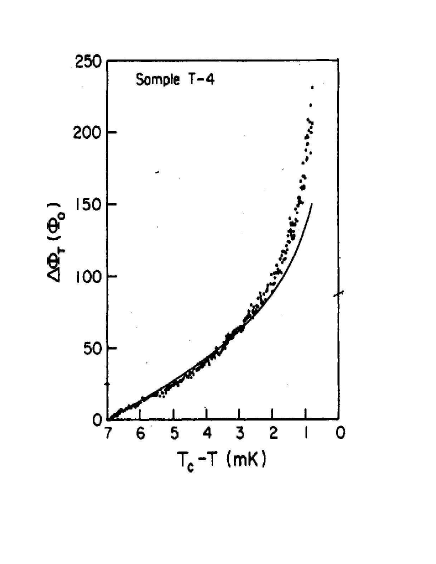
FIG. 2.: Thermally induced magnetic flux in a toroid. The dots are the experimental data of Van Harlingen, Heidel and Garland [16], the line is according to formula (5) of this paper with $T_{1}=T_{\rm c}-7$mK and $T_{2}\equiv T$.

In Fig. 2 we compare experimental data of Van Harlingen, Heidel and Garland [16] with formula (5). The diameters of toroid are $r_{\rm In}=3$ mm and $r_{\rm In}=1$ mm. Material parameters are the thermoelectric coefficient of the normal metal, $L_{T}=9.82~{}10^{3}$ A/Km, and the London penetration depth at the zero temperature, $\lambda_{0}=400$ Å. All the parameters are from Ref. [16] as values for the sample T-4. The only open question is the temperature dependence of the London penetration depth close to the critical temperature $T_{\rm c}^{\rm In}=3.4$ K. We use the asymptotic BCS relation $\lambda=\lambda_{0}/\sqrt{2-2T/T_{\rm c}}$.

In the linear region, $T_{1}-T_{2}\ll T_{\rm c}-T_{2}$, the theory agrees with the experimental data within experimental errors. Perhaps we should return to the original aim of the measurement and conclude that experimental data from [16] confirm that the thermoelectric coefficient $L_{T}$ close below $T_{\rm c}$ has the same value as close above.

In the non-linear region the theory deviates from data. This is no surprise since the presented theory is locally linear in the temperature gradient. Moreover, additional non-linear effects are caused by the so called thermodynamic correction to the electrostatic potential [26, 27]. We aim to discuss these corrections in a next paper.

We should mention that formula (5) has been derived under a tacit assumption that a width $w_{\rm In}$ of the Indium cylinder is sufficiently larger than the London penetration depth $\lambda$. For $\lambda(T_{2})\to w_{\rm In}$ the magnetic flux given by formula (5) approaches $\Phi\to{1\over 2}\Phi_{\rm n}$, where $\Phi_{\rm n}=-\mu_{0}L_{T}(T_{2}-T_{1})w_{\rm In}r_{\rm In}\ln{r_{\rm In}\over r_{\rm Pb}}$. The flux $\Phi_{\rm n}$ develops when the Indium makes transition to the normal (non-superconductive) state, while the Lead remains superconducting. The factor ${1\over 2}$ results from the unrestricted integration of the diamagnetic current into the bulk of Indium valid only for $\lambda\ll w$. Assuming the upper integration limit, $J=\int_{0}^{w}dx\,j$, one finds that $\Phi\to\Phi_{\rm n}$. Unfortunately, details of the flux in the narrow vicinity of $T_{\rm c}$ have not been measured. One can merely speculate that $\Phi_{\rm n}$ is the upper limit of the diverging flux $\Phi$.

Finally, we want to clarify the simple potential matching used above. First, the potential has to match across the whole sample while equation (4) was obtained by matching only at the inner surface. At the outer surface the Bernoulli potential (2) is zero everywhere so that the matching is clearly satisfied. The potential profile between the inner and outer surfaces is nontrivial since the current profile is complicated by itself. Indeed, the screening currents in the Indium and in the Lead spread over different London penetration depths, and they have to match across the whole interface with the current continuity satisfied at each point. We plan to evaluate the current and potential profiles in future. The present theory is based on our believe that the matching at the surface points of the interface is sufficient.

Second, we have ignored the role of the flat pieces in the upper and lower end of sample. In these pieces, the temperature gradient is absent, nevertheless, the potential difference across each piece is nonzero since the current density at the matching corner to the Lead is higher than the current density at the Indium corner. Sending $\nabla T$ to zero in (3) and using obtained velocities in (2), we find that the potential differencies across the upper and the lower flat pieces are identical and thus cancel.

Third, the Bernoulli potential (2) is the simplest approximation of the electrostatic potential. Why we ignore more sophisticated potentials that include the thermodynamic corrections [26] and non-local corrections due to the finite Ginzburg-Landau coherence length [28]? Both these corrections result in a surface dipole [29] which makes the potential matching more complex. On the other hand, with the surface dipole there also appears a dipole at the interface of Indium and Lead. We expect that these dipoles tend to cancel in the final matching condition.

In conclusion, we would like to encourage measurements of thermoelectric coefficients in superconductors. Since the detection of magnetic fluxes is extremely sensitive and fluxes $10^{-3}\Phi_{0}$ can be conveniently monitored, it should be possible to access $L_{T}$ in a wider temperature region, not merely few mK’s bellow $T_{\rm c}$.

Far from $T_{\rm c}$ the present theory is not valid, since the magnetic flux becomes small and it has to exhibit the quantization. Fluxes smaller than the elementary flux are covered by the former theory [3, 4], as confirmed by Zavaritskii [5] and Falco [7], who monitored fluxes of the order of $10^{-2}\Phi_{0}$ and $10^{-1}\Phi_{0}$, respectively.

Interesting features might appear at the intermediate region, where fluxes are comparable to the elementary flux. For instance, the above discussed sample has the classical estimate of thermally induced flux equal to $1\Phi_{0}/$mK at the temperature $T=T_{\rm c}-65$ mK. It should be thus in an access of experiment to observe whether the flux increases in steps $\Phi_{0}$ or smoothly.

We are grateful to Van Harlingen for a kind permission to reproduce their figures. This work was supported by MŠMT program Kontakt ME601 and GAČR 202/03/0410, GAAV A1010312 grants. The European ESF program VORTEX is also acknowledged.

REFERENCES

- [1] von K. Steiner and P. Grassmann, Phys. Z. 36, 527 (1935).
- [2] V. L. Ginzburg, Zh. Eskp. Teor. Phys. 14, 177 (1944) [Sov. Phys. JETP 8, 148 (1944)].
- [3] J. C. Garland and D. J. Van Harlingen, Phys. Lett. 47A, 423 (1974).
- [4] Yu. Gal’perin, V. L. Gurevich and V. I. Kozub, Zh. Eskp. Teor. Phys. 66, 1387 (1974) [Sov. Phys. JETP 39, 680 (1975)].
- [5] N. V. Zavaritskii, Pis’ma Zh. Eskp. Teor. Phys. 19, 205 (1974).
- [6] C. M. Pegrum, A. M. Guénault and G. R. Pickett, in Proceedings of the 14th International Conference Low Temperature Physicsm Otaniemi, Finland 1975, edited by M. Krusius and M. Vurio (Noth-Holland, Amsterdam 1975), Vol. 2, p. 513.
- [7] C. M. Falco, Solid State Commun. 19, 623 (1976).
- [8] D. J. Van Harlingen and J. C. Garland, Solid State Commun. 25, 419 (1978).
- [9] A. A. Matsinger, R. de Bruyn Outboter and H. van Beelen, Physica 93B, 63 (1977).
- [10] C. M. Pegrum and A. M. Guénault, Phys. Lett. 59A, 393 (1976).
- [11] L. Z. Kon, Zh. Eskp. Teor. Phys. 70, 286 (1976) [Sov. Phys. JETP 43, 149 (1976)].
- [12] S. N. Artemenko and A. F. Volkov, Zh. Eskp. Teor. Phys. 70, 1051 (1976) [Sov. Phys. JETP 43, 548 (1976)].
- [13] V. I. Kozub, Zh. Eskp. Teor. Phys. 74, 344 (1978) [Sov. Phys. JETP 47, 178 (1978)].
- [14] D. F. Heidel and J. C. Garland, J. Phys. (Paris) 39, C6-492 (1978).
- [15] R. A. Sacks, J. Low. Temp. Phys. 34, 393 (1979).
- [16] D. J. Van Harlingen, D. F. Heidel and J. C. Garland, Phys. Rev. B 21, 1842 (1980).
- [17] C. M. Falco, Phys. Rev. Lett. 39, 660 (1977).
- [18] H. J. Mamin, J. Clarke and D. J. Van Harlingen, Phys. Rev. B 29, 3881 (1984).
- [19] D. C. Marinescu and A. W. Overhauser, Phys. Rev. B 55, 11637 (1997).
- [20] J. Bardeen, G. Rickayzen and L. Tewordt, Phys. Rev. 113, 982 (1959).
- [21] Y. M. Gal’perin, V. L. Gurevich, V. I. Kozub and A. L. Shelankov, Phys. Rev. B 65, 064531 (2002).
- [22] A. G. van Vijfeijken and F. S. Staas, Phys. Lett. 12, 175 (1964).
- [23] J. Bok and J. Klein, Phys. Rev. Lett. 20, 660 (1968).
- [24] J. B. Brown and T. D. Morris, Proc. 11th Int. Conf. Low. Temp. Phys., Vol. 2, 768 (St. Andrews, 1968).
- [25] T. D. Morris and J. B. Brown, Physica 55, 760 (1971).
- [26] G. Rickayzen, J. Phys. C 2, 1334 (1969).
- [27] P. Lipavský, J. Koláček, K. Morawetz and E. H. Brandt, Phys. Rev. B 65, 144511 (2002).
- [28] P. Lipavský, K. Morawetz, J. Koláček, J. J. Mareš, E. H. Brandt and M. Schreiber, Phys. Rev. B 69, 024524 (2004).
- [29] P. Lipavský, J. Koláček and J. J. Mareš, K. Morawetz, Phys. Rev. B 65, 012507 (2001).