Formation of charge-stripe phases in a system of spinless fermions or hardcore bosons

Abstract

We consider two strongly correlated two-component quantum systems, consisting of quantum mobile particles and classical immobile particles. The both systems are described by Falicov–Kimball-like Hamiltonians on a square lattice, extended by direct short-range interactions between the immobile particles. In the first system the mobile particles are spinless fermions while in the second one they are hardcore bosons. We construct rigorously ground-state phase diagrams of the both systems in the strong-coupling regime and at half-filling. Two main conclusions are drawn. Firstly, short-range interactions in quantum gases are sufficient for the appearance of charge stripe-ordered phases. By varying the intensity of a direct nearest-neighbor interaction between the immobile particles, the both systems can be driven from a phase-separated state (the segregated phase) to a crystalline state (the chessboard phase) and these transitions occur necessarily via charge-stripe phases: via a diagonal striped phase in the case of fermions and via vertical (horizontal) striped phases in the case of hardcore bosons. Secondly, the phase diagrams of the two systems (mobile fermions or mobile hardcore bosons) are definitely different. However, if the strongest effective interaction in the fermionic case gets frustrated gently, then the phase diagram becomes similar to that of the bosonic case.

and

1 Introduction

In the passing decade, some specific phases, having quasi-one-dimensional structure, the so called striped phases, have been a highly debated subject in condensed-matter physics. Apparently, a broad interest in such phases was initiated by reports presenting experimental evidence for the existence of charge strips in doped layered perovskites, some of which constitute materials exhibiting high-temperature superconductivity [1, 2].

However, striped phases had been observed much earlier, for instance on metallic surfaces covered with an adsorbate, see [3] and references therein. Theoretical descriptions of these phenomena involved various kinds of lattice gas models [4]. Many other instances of experimental observations of stripe-ordered phases are listed in [5], where Monte-Carlo studies of formation of striped phases in a continuous gas with hardcore and short-range repulsive interactions are reported.

Quite interestingly, theoretical studies of striped phases in systems of strongly correlated electrons have preceded experimental observations of such phases [6, 7]. But only after those observations, the discussion became much more vigorous, and the nature of stripe-ordered phases started to attract attention of numerous researchers. In the context of the Hubbard model, a comprehensive review of the problem can be found in [8]. The existence of the same kind of striped phases was investigated also in the $t$–$J$ model [9, 10]. A bird’s eye view on the problem of stripe-ordered phases in high-temperature superconductors, but emphasizing its general relevance for contemporary condensed-matter physics can be found in [11]. The general relevance of striped phases is underlined also in [12], where they are viewed as an emergent phenomenon resulting from collective motions of microscopic particles, somewhat analogous to quasi-particles like phonons. Striped phases have been also studied in the framework of quantum-spin models, like $XY$ model for instance [13].

The Hubbard or $t$–$J$-like models belong to the most realistic models, in the framework of which the problem of striped-ordered phases in doped layered perovskites can be investigated. In the both models, the spin and the charge degrees of freedom are taken into account, and it is believed that it is the competition between these degrees of freedom that is decisive for the formation of striped phases. The question of formation of striped phases is closely related to the question of relative stability of these phases against mixtures of an electron-reach phase and a hole-reach phase. Due to the tiny energy differences between both phases, the results obtained by means of approximate methods, which introduce hardly-controllable errors, are disparate. And this can be said despite, as emphasized in [8], a spectacular consensus of results concerning half-filled stripes, obtained by means of various approximate methods. Therefore, as pointed out in [12, 15] further careful studies are necessary to settle the problem of formation of stripe-ordered phases. One of possible ways of attacking this problem is to formulate analog problems in less realistic but simpler models, where some control over the results obtained by means of various methods of many-body physics can be gained. This leads hopefully to a deeper insight into the, mentioned above, stability problem.

Such an approach has been adopted by many researchers, see for instance [12, 14, 15, 16, 17]. Buhler et al [14] have found, by means of Monte Carlo simulations, that upon hole doping antiferromagnetic spin domains and charge stripes, whose properties are in very good agreement with experiments, appear in a spin-fermion model for cuprates. Using the so called restricted phase diagrams, the stability problem of charge-stripe phases has been studied in the spinless Falicov–Kimball model by Lemanski et al [15, 16]. In their study the formation of charge stripe-ordered phases can be looked upon as a way the system interpolates between a periodic charge-density wave phase (the chessboard phase) and the segregated phase (a mixture of completely filled and completely empty phases), as the degree of doping varies. A considerable reduction of the Hilbert space dimension in a spinless fermion model with infinite nearest-neighbor repulsion (as compared to a Hubbard model) has been exploited by Zhang and Henley [12, 17] to study carefully, by means of an exact diagonalization technique, the formation of charge stripe-ordered phases upon doping. They addressed also an interesting question of the role of quantum statistics in the problem of striped phases, by replacing fermion particles with hardcore boson ones.

Our work has been inspired mainly by the recent studies of Lemański et al [15, 16] and by Zhang and Henley [12, 17]. To investigate the key question, whether charge stripe-ordered phases are stable compared to a phase-separated state, we study rigorously the strong-coupling limit of an extended spinless Falicov–Kimball model on a square lattice, with mobile particles being spinless fermions or hardcore bosons. The usual spinless Falicov–Kimball Hamiltonian (such as that studied in [18]) has been augmented by a direct, Ising-like, interaction between the immobile particles.

To explain the role played by the extra interaction we have to make a few remarks. Firstly, for technical reasons, our analysis is restricted to the case of half-filling. Secondly, it is now well established (proven) [18, 19] that, in the fermion spinless Falicov–Kimball model the phase-separated state, the segregated phase, is stable only off the half-filling. Thus, an additional interaction is needed to stabilize the segregated phase at half-filling. Thirdly, in the regime of singly occupied sites and for strong-coupling, the strongest effective interaction in the Hubbard model is the Heisenberg antiferromagnetic interaction. Doping of holes can be seen as means to weaken the strong tendency toward antiferromagnetic ordering and to make possible a phase separated state with hole-reach and electron-reach regions. Under similar conditions, in the spinless Falicov–Kimball model an analogous role is played by the Ising-like nearest-neighbor (n.n.) repulsive interaction between the immobile particles that favors a chessboard-like ordering. The effect of weakening of the strong tendency toward chessboard ordering can be achieved by an extra Ising-like n.n. interaction that compensates the strongest repulsive interaction, and consequently permits the system to reach a phase-separated state, the segregated phase. On varying, in a suitable interval of values, the corresponding interaction constant, which is our control parameter, we can study how the both systems “evolve” from the crystalline chessboard phase to the segregated one.

We prove that by varying the interaction constant of the direct n.n. interaction between the immobile particles, the both systems (fermion and boson) can be driven, via a sequence of phase transitions, from a crystalline state (the chessboard phase) to a phase-separated state (the segregated phase). Moreover, these transitions occur necessarily via charge-stripe phases: via a diagonal striped phase in the case of fermions and via vertical (horizontal) striped phases in the case of hardcore bosons. Thus, short-range interactions in quantum gases are sufficient for the appearance of charge stripe-ordered phases.

In our studies, we include also a subsidiary direct interaction between the immobile particles, an Ising-like next nearest-neighbor (n.n.n.) interaction, much weaker than the n.n. interaction. This interaction can reinforce or frustrate the n.n. interaction, depending on the sign of its interaction constant. It appears that on varying the control parameter (the strength of n.n. interactions), the systems (fermion or boson) characterized by different values of n.n.n. interactions, may undergo different sequences of transitions between the chessboard phase and the segregated one. We find, in particular, that if we set appropriate values of the n.n.n. interaction in the fermion system and in the boson one, then the both systems settle in the same phases, for typical values of the control parameter. On the other hand, the n.n.n. interaction enables us to demonstrate that the ground-state phase diagrams in the cases of mobile fermions and mobile hardcore bosons are definitely different.

As a byproduct of our considerations, we obtain an Ising-like short-range Hamiltonian, with pair interactions at distance of two lattice constants and four-site (plaquette) interactions, whose ground states consist of stripe-like configurations or chessboard-like configurations, depending on the sign of the unique coupling constant. These ground states are stable with respect to perturbations by n.n. and n.n.n. interactions.

The paper is organized as follows. In the next section we present the considered models and general properties of the corresponding Hamiltonians. Then, in section 3 we construct phase diagrams due to truncated effective interactions. After that, in section 4, we analyze the phase diagrams due to complete interactions (without truncation) of the both quantum systems studied here and formulate our conclusions. Finally, in section 5, we summarize our results.

2 The model and its basic properties

The model to be studied is a simplified version of the one band, spin $1/2$ Hubbard model, known as the static approximation (one sort of electrons hops while the other sort is immobile), augmented by a direct Ising-like interaction $V$ between the immobile particles. Thus the total Hamiltonian of the system reads:

$$H_{0}=H_{FK}+V,$$ (1)

$$H_{FK}=-t\sum\limits_{\langle x,y\rangle_{1}}\,\left(c^{+}_{x}c_{y}+c^{+}_{y}c_{x}\right)+U\sum\limits_{x}\left(c^{+}_{x}c_{x}-\frac{1}{2}\right)s_{x},$$ (2)

$$V=\frac{W}{8}\sum\limits_{\langle x,y\rangle_{1}}s_{x}s_{y}-\frac{\tilde{\varepsilon}}{16}\sum\limits_{\langle x,y\rangle_{2}}s_{x}s_{y}.$$ (3)

In the above formulae, the underlying lattice is a square lattice, denoted $\Lambda$, consisting of sites $x,y,\ldots$, whose number is $|\Lambda|$, having the shape of a $\sqrt{|\Lambda|}\times\sqrt{|\Lambda|}$ torus. In (2,3) and below, the sums $\sum_{\langle x,y\rangle_{i}}$, $i=1,2,3$, stand for the summation over all the $i$-th order n.n. pairs of lattice sites in $\Lambda$, with each pair counted once.

The subsystem of mobile spinless particles is described in terms of creation and annihilation operators of an electron at site $x$: $c^{+}_{x}$, $c_{x}$, respectively, satisfying the canonical anticommutation relations (spinless electrons) or the commutation relations of spin $1/2$ operators $S^{+}_{x},S^{-}_{x},S^{z}_{x}$ (hardcore bosons). The total electron-number (boson-number) operator is $N_{e}=\sum_{x}c^{+}_{x}c_{x}$, and (with a little abuse of notation) the corresponding electron (boson) density is $\rho_{e}=N_{e}/|\Lambda|$. There is no direct interaction between mobile particles. Their energy is due to hopping, with $t$ being the n.n. hopping intensity, and due to the interaction with the localized particles, whose strength is controlled by the coupling constant $U$.

The subsystem of localized particles (here-after called ions), is described by a collection of pseudo-spins $\left\{s_{x}\right\}_{x\in\Lambda}$, with $s_{x}=1,-1$ ($s_{x}=1$ if the site $x$ is occupied by an ion and $s_{x}=-1$ if it is empty), called the ion configurations. The total number of ions is $N_{i}=\sum_{x}(s_{x}+1)/2$ and the ion density is $\rho_{i}=N_{i}/|\Lambda|$. In our model the ions interact directly, with energy given by $V$.

Clearly, in the composite system, whose Hamiltonian is given by (1), with arbitrary electron-ion (boson-ion) coupling $U$, the particle-number operators $N_{e}$, $N_{i}$, and pseudo-spins $s_{x}$, are conserved. Therefore the description of the classical subsystem in terms of the ion configurations $S=\left\{s_{x}\right\}_{x\in\Lambda}$ remains valid. Whenever periodic configurations of pseudo-spins are considered, it is assumed that $\Lambda$ is sufficiently large, so that it accommodates an integer number of elementary cells.

Nowadays, $H_{FK}$ is widely known as the Hamiltonian of the spinless Falicov–Kimball model, a simplified version of the Hamiltonian put forward in [20]. To the best of our knowledge, the spinless-fermion Falicov–Kimball model is the unique system of interacting fermions, for which the existence of a long-range order (the chessboard phase) [21, 22] and of a phase separation (the segregated phase) [18, 19] have been proved. A review of other rigorous results and an extensive list of relevant references can be found in [23, 24]).

In what follows, we shall study the ground-state phase diagram of the system defined by (1) in the grand-canonical ensemble. That is, let

$$H\left(\mu_{e},\mu_{i}\right)=H_{0}-\mu_{e}N_{e}-\mu_{i}N_{i},$$ (4)

where $\mu_{e}$, $\mu_{i}$ are the chemical potentials of the electrons (bosons) and ions, respectively, and let $E_{S}\left(\mu_{e},\mu_{i}\right)$ be the ground-state energy of $H\left(\mu_{e},\mu_{i}\right)$, for a given configuration $S$ of the ions. Then, the ground-state energy of $H\left(\mu_{e},\mu_{i}\right)$, $E_{G}\left(\mu_{e},\mu_{i}\right)$, is defined as $E_{G}\left(\mu_{e},\mu_{i}\right)=\min\left\{E_{S}\left(\mu_{e},\mu_{i}\right):S\right\}$. The minimum is attained at the set $G$ of the ground-state configurations of ions. We shall determine the subsets of the $\left(\mu_{e},\mu_{i}\right)$-plane, where $G$ consists of periodic configurations of ions, uniformly in the size of the underlying square lattice.

In studies of grand-canonical phase diagrams an important role is played by unitary transformations (hole–particle transformations) that exchange particles and holes, $c^{+}_{x}c_{x}\rightarrow 1-c^{+}_{x}c_{x}$, $s_{x}\rightarrow-s_{x}$, and for some $\left(\mu^{0}_{e},\mu^{0}_{i}\right)$ leave the Hamiltonian $H\left(\mu_{e},\mu_{i}\right)$ invariant. For the mobile particles such a role is played by the transformations: $c_{x}^{+}\rightarrow\epsilon_{x}c_{x}$, where $\epsilon_{x}=1$ for bosons while for fermions $\epsilon_{x}=1$ at the even sublattice of $\Lambda$ and $\epsilon_{x}=-1$ at the odd one. Clearly, since $H_{0}$ is invariant under the joint hole–particle transformation of mobile and localized particles, $H\left(\mu_{e},\mu_{i}\right)$ is hole–particle invariant at the point $(0,0)$. At the hole–particle symmetry point, the system under consideration has very special properties, which simplify studies of its phase diagram [22]. Moreover, by means of the defined above hole-particle transformations one can determine a number of symmetries of the grand-canonical phase diagram [25]. The peculiarity of the model is that the case of attraction ($U<0$) and the case of repulsion ($U>0$) are related by a unitary transformation (the hole-particle transformation for ions): if $S=\left\{s_{x}\right\}_{x\in\Lambda}$ is a ground-state configuration at $\left(\mu_{e},\mu_{i}\right)$ for $U>0$, then $-S=\left\{-s_{x}\right\}_{x\in\Lambda}$ is the ground-state configuration at $\left(\mu_{e},-\mu_{i}\right)$ for $U<0$. Consequently, without any loss of generality one can fix the sign of the coupling constant $U$. Moreover (with the sign of $U$ fixed), there is an inversion symmetry of the grand-canonical phase diagram, that is, if $S$ is a ground-state configuration at $\left(\mu_{e},\mu_{i}\right)$, then $-S$ is the ground-state configuration at $\left(-\mu_{e},-\mu_{i}\right)$. Therefore, it is enough to determine the phase diagram in a half-plane specified by fixing the sign of one of the chemical potentials.

Our aim in this paper is to investigate the ground-state phase diagrams of our systems, for general values of the energy parameters that appear in $H\left(\mu_{e},\mu_{i}\right)$. According to the state of art, this is feasible only in the strong-coupling regime, i.e. when $|t/U|$ is sufficiently small. Therefore, from now on we shall consider exclusively the case of a large positive coupling $U$, and we express all the parameters of $H\left(\mu_{e},\mu_{i}\right)$ in the units of $U$, preserving the previous notation.

In the strong-coupling regime, the ground-state energy $E_{S}\left(\mu_{e},\mu_{i}\right)$ can be expanded in a power series in $t$. One of the ways to achieve this, for fermions and for hardcore bosons, is a closed-loop expansion [26, 27]. The result, with the expansion terms up to order four shown explicitly, reads:

$$E^{fermion}_{S}\left(\mu_{e},\mu_{i}\right) = -\frac{1}{2}\left(\mu_{i}-\mu_{e}\right)\sum\limits_{x}s_{x}-\frac{1}{2}\left(\mu_{i}+\mu_{e}+1\right)|\Lambda|+$$ (5)

$$\left[\frac{t^{2}}{4}-\frac{9t^{4}}{16}+\frac{W}{8}\right]\sum\limits_{\langle x,y\rangle_{1}}s_{x}s_{y}+\left[\frac{3t^{4}}{16}-\frac{\tilde{\varepsilon}}{16}\right]\sum\limits_{\langle x,y\rangle_{2}}s_{x}s_{y}+$$

$$\frac{t^{4}}{8}\sum\limits_{\langle x,y\rangle_{3}}s_{x}s_{y}+\frac{t^{4}}{16}\sum\limits_{P}\left(1+5s_{P}\right)+R^{(4)},$$

for fermions, and

$$E^{boson}_{S}\left(\mu_{e},\mu_{i}\right) = -\frac{1}{2}\left(\mu_{i}-\mu_{e}\right)\sum\limits_{x}s_{x}-\frac{1}{2}\left(\mu_{i}+\mu_{e}+1\right)|\Lambda|+$$ (6)

$$\left[\frac{t^{2}}{4}-\frac{5t^{4}}{16}+\frac{W}{8}\right]\sum\limits_{\langle x,y\rangle_{1}}s_{x}s_{y}+\left[\frac{5t^{4}}{16}-\frac{\tilde{\varepsilon}}{16}\right]\sum\limits_{\langle x,y\rangle_{2}}s_{x}s_{y}+$$

$$\frac{t^{4}}{8}\sum\limits_{\langle x,y\rangle_{3}}s_{x}s_{y}-\frac{t^{4}}{16}\sum\limits_{P}\left(5+s_{P}\right)+{\tilde{R}}^{(4)},$$

for hardcore bosons, up to a term independent of the ion configuration and the chemical potentials. In (5) and (6), $P$ denotes the $(2\times 2)$-plaquette of the square lattice $\Lambda$, $s_{P}$ stands for the product of pseudo-spins assigned to the corners of $P$, and the remainders $R^{(4)}$, ${\tilde{R}}^{(4)}$, which are independent of the chemical potentials and the parameters $W$ and $\tilde{\varepsilon}$, collect those terms of the expansion that are proportional to $t^{2m}$, with $m=3,4,\ldots$. It can be proved that the above expansions are absolutely convergent, uniformly in $\Lambda$, provided that $t<1/16$ and $\left|\mu_{e}\right|<1-16t$ [26, 27]. Moreover, under these conditions the particle densities satisfy the half-filling relation: $\rho_{e}+\rho_{i}=1$.

3 Phase diagrams according to truncated expansions

We note that on taking into account the inversion symmetry of the phase diagram in the $\left(\mu_{e},\mu_{i}\right)$-plane and the fact that the ground-state energies depend only on the difference of the chemical potentials, in order to determine the phase diagram in the stripe $\left|\mu_{e}\right|<1-16t$ it is enough to consider the phase diagram at the half-line $\mu_{e}=0$, $\mu_{i}<0$ (or $\mu_{i}>0$). At this half-line we set $\mu_{i}\equiv\mu$.

Due to the convergence of the expansions (5) and (6), it is possible to establish rigorously a part of the phase diagram (that is the ground-state configurations of ions are determined everywhere in the $\left(\mu_{e},\mu_{i}\right)$-plane, except some small regions), by determining the phase diagram of the expansion truncated at the order $k$, that is according to the $k$-th order effective Hamiltonians $(E^{fermion}_{S})^{(k)}\left(0,\mu\right)$ and $(E^{boson}_{S})^{(k)}\left(0,\mu\right)$. In order to construct a phase diagram according to a $k$-th order effective Hamiltonian, we use the $m$-potential method introduced in [28], with technical developments described in [25, 29, 27].

3.1 The zeroth and second order ground-state phase diagrams

An inspection of (5) and (6) reveals that up to the second order the effective Hamiltonians for fermions and hardcore bosons are the same. Hence, the discussion that follows applies to the both cases, and the common effective Hamiltonians are denoted as $E_{S}^{(0)}\left(0,\mu\right)$, $E_{S}^{(2)}\left(0,\mu\right)$.

In the zeroth order,

$$E_{S}^{(0)}\left(0,\mu\right) = -\frac{\mu}{2}\sum\limits_{x}\left(s_{x}+1\right)+\frac{W}{8}\sum\limits_{\langle x,y\rangle_{1}}s_{x}s_{y}-\frac{\tilde{\varepsilon}}{16}\sum\limits_{\langle x,y\rangle_{2}}s_{x}s_{y}$$ (7)

$$= \sum\limits_{P}H_{P}^{(0)},$$

where

$$H_{P}^{(0)}=-\frac{\mu}{8}\sideset{}{{}^{\prime}}{\sum}\limits_{x}\left(s_{x}+1\right)+\frac{W}{16}\sideset{}{{}^{\prime}}{\sum}\limits_{\langle x,y\rangle_{1}}s_{x}s_{y}-\frac{\tilde{\varepsilon}}{16}\sideset{}{{}^{\prime}}{\sum}\limits_{\langle x,y\rangle_{2}}s_{x}s_{y},$$ (8)

and the primed sums in (8) are restricted to a plaquette $P$. For any $\tilde{\varepsilon}>0$, the plaquette potentials $H_{P}^{(0)}$ are minimized by the restrictions to a plaquette $P$ of a few periodic configurations of ions on $\Lambda$. Namely, $S_{-}$ — the empty configuration ($S_{+}$ — the completely filled configuration), where $s_{x}=-1$ at every site ($s_{x}=+1$ at every site), and the chessboard configurations $S_{cb}^{e}$, where $s_{x}=\epsilon_{x}$, and $S_{cb}^{o}$ (where $s_{x}=-\epsilon_{x}$), with $\epsilon_{x}=1$ if $x$ belongs to the even sublattice of $\Lambda$ and $\epsilon_{x}=-1$ otherwise. Moreover, out of the restrictions of those configurations to a plaquette $P$, $S_{-|P}$, $S_{+|P}$, $S^{e}_{cb|P}$, and $S_{cb|P}^{o}$, only four ground-state configurations on $\Lambda$ can be built, which coincide with the four configurations named above. Clearly, this is due to the direct n.n.n. attractive interaction between the ions. The section of the phase diagram in the $(W,\mu,\tilde{\varepsilon})$ space by a plane with $\tilde{\varepsilon}>0$, according to the effective Hamiltonian $E^{(0)}_{S}\left(0,\mu\right)$, is shown in Fig. 2.

Figure 1: Ground-state phase diagram of $E^{(0)}_{S}\left(0,\mu\right)$ for fermion and hard-core boson systems.

Figure 2: Ground-state phase diagram of $E^{(2)}_{S}\left(0,\mu\right)$ for fermion and hard-core boson systems.

In the second order,

$$E_{S}^{(2)}\left(0,\mu\right) = -\frac{\mu}{2}\sum\limits_{x}\left(s_{x}+1\right)+\left[\frac{t^{2}}{4}+\frac{W}{8}\right]\sum\limits_{\langle x,y\rangle_{1}}s_{x}s_{y}-\frac{\tilde{\varepsilon}}{16}\sum\limits_{\langle x,y\rangle_{2}}s_{x}s_{y}$$ (9)

$$= \sum\limits_{P}H_{P}^{(2)},$$

where $H_{P}^{(2)}$,

$$H_{P}^{(2)}=-\frac{\mu}{8}\sideset{}{{}^{\prime}}{\sum}\limits_{x}\left(s_{x}+1\right)+\left[\frac{t^{2}}{8}+\frac{W}{16}\right]\sideset{}{{}^{\prime}}{\sum}\limits_{\langle x,y\rangle_{1}}s_{x}s_{y}-\frac{\tilde{\varepsilon}}{16}\sideset{}{{}^{\prime}}{\sum}\limits_{\langle x,y\rangle_{2}}s_{x}s_{y},$$ (10)

and the primed sums are restricted to a plaquette $P$. Since $E_{S}^{(2)}$ differs from $E_{S}^{(0)}$ by the strength of n.n. interactions, the only effect on the phase diagram is that the coexistence lines are translated by the vector $(-2t^{2},0,0)$. The section of the phase diagram in the $(W,\mu,\tilde{\varepsilon})$ space by a plane with $\tilde{\varepsilon}>0$, according to the effective Hamiltonian $E^{(2)}_{S}\left(0,\mu\right)$, is shown in Fig. 2.

3.2 The fourth order ground-state phase diagrams

It follows from the investigation of the phase diagram up to the second order that the degeneracy is finite, independently of the size of $\Lambda$, everywhere except the coexistence lines in the ($\tilde{\varepsilon}=0$)-plane, where it grows exponentially with $|\Lambda|$. Only there the effect of the fourth order interactions can be most significant. The meeting point of the coexistence lines in the ($\tilde{\varepsilon}=0$)-plane, where the coexistence line of $S_{+}$ and $S_{-}$ sticks to the stability domain of chessboard configurations, appears to be particularly interesting. In that point, the energies of all the configurations are the same. In what follows, we shall study the phase diagrams of spinless fermions and spinless hardcore bosons up to the fourth order, in a neighborhood of radius $O(t^{4})$ of the point $(-2t^{2},0,0)$. In this neighborhood, it is convenient to introduce new coordinates, $(W,\mu,\tilde{\varepsilon})\to(\omega,\delta,\varepsilon)$,

$$W=-2t^{2}+t^{4}\omega,\hskip 14.22636pt\mu=t^{4}\delta,\hskip 14.22636pt\tilde{\varepsilon}=t^{4}\varepsilon,$$ (11)

and a new (equivalent to $(E^{fermion}_{S})^{(4)}$) $t$-independent effective Hamiltonian, $(H^{fermion}_{{\mathrm{eff}}})^{(4)}$,

$$(E^{fermion}_{S})^{(4)}\left(0,\delta\right)=\frac{t^{4}}{2}(H^{fermion}_{{\mathrm{eff}}})^{(4)}.$$ (12)

Then, in the spirit of the $m$-potential method, we express $(H^{fermion}_{{\mathrm{eff}}})^{(4)}$ by the potentials $(H^{fermion}_{T})^{(4)}$,

$$(H^{fermion}_{{\mathrm{eff}}})^{(4)}=\sum\limits_{T}(H^{fermion}_{T})^{(4)},$$ (13)

where, in terms of the new variables,

$$(H^{fermion}_{T})^{(4)} = -\delta\left(s_{5}+1\right)+\frac{1}{24}\left(\omega-\frac{9}{2}\right)\sideset{}{{}^{\prime\prime}}{\sum}\limits_{\langle x,y\rangle_{1}}s_{x}s_{y}+\frac{1}{32}\left(3-\varepsilon\right)\sideset{}{{}^{\prime\prime}}{\sum}\limits_{\langle x,y\rangle_{2}}s_{x}s_{y}+$$ (14)

$$\frac{1}{12}\sideset{}{{}^{\prime\prime}}{\sum}\limits_{\langle x,y\rangle_{3}}s_{x}s_{y}+\frac{1}{32}\sideset{}{{}^{\prime\prime}}{\sum}\limits_{P}\left(5s_{P}+1\right).$$

In (13) and (14), $T$ stands for a $(3\times 3)$-plaquette (later on called the $T$-plaquette) of a square lattice, whose sites are labeled from the left to the right, starting at the bottom left corner and ending in the upper right one. Consequently, $s_{5}$ is the pseudo-spin of the central site. The double-primed sums are restricted to a $T$-plaquette. For bosons, we introduce $(H^{boson}_{{\mathrm{eff}}})^{(4)}$ and $(H^{boson}_{T})^{(4)}$ in the same manner as for fermions, with

$$(H^{boson}_{T})^{(4)} = -\delta\left(s_{5}+1\right)+\frac{1}{24}\left(\omega-\frac{5}{2}\right)\sideset{}{{}^{\prime\prime}}{\sum}\limits_{\langle x,y\rangle_{1}}s_{x}s_{y}+\frac{1}{32}\left(5-\varepsilon\right)\sideset{}{{}^{\prime\prime}}{\sum}\limits_{\langle x,y\rangle_{2}}s_{x}s_{y}+$$ (15)

$$\frac{1}{12}\sideset{}{{}^{\prime\prime}}{\sum}\limits_{\langle x,y\rangle_{3}}s_{x}s_{y}-\frac{1}{32}\sideset{}{{}^{\prime\prime}}{\sum}\limits_{P}\left(s_{P}+5\right).$$

By the remark at the begining of this section, we have to search for the lowest-energy configurations of $(E^{fermion}_{S})^{(4)}$ and $(E^{boson}_{S})^{(4)}$ among all the configurations. Consequently, the potentials $(H^{fermion}_{T})^{(4)}$ and $(H^{boson}_{T})^{(4)}$ have to be minimized over all the $T$-plaquette configurations. There are (up to the symmetries of $H_{0}$) 102 different $T$-plaquette configurations, shown in Fig. 3.

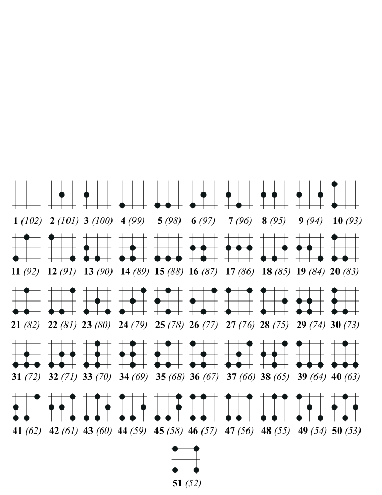
Figure 3: All the $T$-plaquette configurations, up to the symmetries of $H_{0}$. The configurations that can be obtained from the displayed ones by the hole-particle transformation are not shown, only the numbers assigned to them are given in brackets.

Unfortunately, in contrast to the lower-order cases, the potentials $(H^{fermion}_{T})^{(4)}$ and $(H^{boson}_{T})^{(4)}$ turn out to be the $m$-potentials only in a small part of $(\omega,\delta,\varepsilon)$-space. This difficulty can be overcome by introducing the so called zero-potentials [25, 29, 27], denoted $K_{T}^{(4)}$, that are invariant with respect to the symmetries of $H_{0}$ and satisfy the condition

$$\sum\limits_{T}K_{T}^{(4)}=0.$$ (16)

Following [29], $K_{T}^{(4)}$ are chosen in the form

$$K^{(4)}_{T}=\sum\limits_{i=1}^{5}\alpha_{i}k_{T}^{(i)},$$ (17)

where the coefficients $\alpha_{i}$, depending on $(\omega,\delta,\varepsilon)$ in general, have to be determined in the process of constructing the phase diagram, and the potentials $k_{T}^{(i)}$ are defined by

$$k_{T}^{(1)} = s_{1}+s_{3}+s_{7}+s_{9}-4s_{5},$$

$$k_{T}^{(2)} = s_{2}+s_{4}+s_{6}+s_{8}-4s_{5},$$

$$k_{T}^{(3)} = s_{1}s_{2}+s_{2}s_{3}+s_{3}s_{6}+s_{6}s_{9}+s_{8}s_{9}+s_{7}s_{8}+s_{4}s_{7}+s_{1}s_{4}$$

$$-2s_{2}s_{5}-2s_{5}s_{6}-2s_{5}s_{8}-2s_{4}s_{5},$$

$$k_{T}^{(4)} = s_{1}s_{5}+s_{3}s_{5}+s_{5}s_{9}+s_{5}s_{7}-s_{2}s_{4}-s_{4}s_{8}-s_{8}s_{6}-s_{2}s_{6},$$

$$k_{T}^{(5)} = s_{1}s_{3}+s_{3}s_{9}+s_{7}s_{9}+s_{1}s_{7}-2s_{4}s_{6}-2s_{2}s_{8}.$$ (18)

Note that the potentials $k_{T}^{(i)}$ are invariant with respect to the symmetries of $H_{0}$ and they satisfy (16), therefore these properties are shared by the potentials $K^{(4)}_{T}$.

By means of the zero-potentials $K^{(4)}_{T}$, new candidates for $m$-potentials can be introduced,

$$(H^{fermion}_{{\mathrm{eff}}})^{(4)}=\sum\limits_{T}\left((H^{fermion}_{T})^{(4)}+K^{(4)}_{T}\right),$$ (19)

with an analogous representation of $(H^{boson}_{{\mathrm{eff}}})^{(4)}$, and now the task is to minimize the potentials $(H^{fermion}_{T})^{(4)}+K^{(4)}_{T}$and $(H^{boson}_{T})^{(4)}+K^{(4)}_{T}$ over all the $T$-plaquette configurations.

In our study of the ground-state phase diagrams we limit ourselves to the ($\delta=0$)-plane, where the both considered systems are hole-particle invariant, and to the ($\varepsilon=0$)-plane. Our analysis of the minima of the $T$-plaquette potentials, $(H^{fermion}_{T})^{(4)}$ and $(H^{boson}_{T})^{(4)}$ augmented by the zero-potentials $K^{(4)}_{T}$, shows that these planes are partitioned into a finite number of open domains ${\mathcal{S}}_{D}$, each with its unique set of periodic ground-state configurations on $\Lambda$, denoted also by ${\mathcal{S}}_{D}$. There is a finite number, independent of $|\Lambda|$, of configurations in ${\mathcal{S}}_{D}$ and they are related by the symmetries of $H_{0}$. The last two statements do not apply to only one of the domains, denoted ${\mathcal{S}}_{d2}$, which will be described in the sequel.

The domains ${\mathcal{S}}_{D}$ are characterized as follows: at each point $p$ ($p=(\omega,\varepsilon)$ or $p=(\omega,\delta)$) of a domain ${\mathcal{S}}_{D}$, there exist a set of coefficients $\left\{\alpha_{i}(p)\right\}$ such that the corresponding potentials are minimized by a set ${\mathcal{S}}_{TD}(p)$ of $T$-plaquette configurations. Moreover, from the configurations in ${\mathcal{S}}_{TD}(p)$ one can construct only the configurations in ${\mathcal{S}}_{D}$. The set of the restrictions to $T$-plaquettes of the configurations from ${\mathcal{S}}_{D}$, ${\mathcal{S}}_{D|T}$, is contained in each set ${\mathcal{S}}_{TD}(p)$ with $p\in{\mathcal{S}}_{D}$. In Table 4 of Appendix we mark by asterisk the cases, where the set ${\mathcal{S}}_{TD}(p)$ contains, besides ${\mathcal{S}}_{D|T}$, some additional $T$-plaquette configurations.

Specifically, for $\delta=0$ the ground-state phase diagrams due to the effective Hamiltonians $(H^{fermion}_{{\mathrm{eff}}})^{(4)}$ and $(H^{boson}_{{\mathrm{eff}}})^{(4)}$ are shown in Fig. 5 and Fig. 5,

Figure 4: The ($\mu=0$)-phase diagram of the effective Hamiltonian $(H^{fermion}_{{\mathrm{eff}}})^{(4)}$. The numbers in curly brackets, displayed by the symbols of open domains ${\mathcal{S}}_{D}$, denote the $T$-plaquette configurations that minimize the $m$-potential in ${\mathcal{S}}_{D}$. The numbers in curly brackets, displayed by the boundary-line segments or by the arrows pointing towards boundary segments (or their crossing points) identify the additional minimizing $T$-plaquette configurations. For more comments see the text. The boundary-line segments can be determined by means of their intersection points: ${\bf a}=(9/2,12)$, ${\bf b}=(-5/2,-2)$, ${\bf c}=(23/2,-2)$, ${\bf d}=(-5/2,-6)$, ${\bf e}=(23/2,-6)$, and by the slope $1$ of the boundary of ${\mathcal{S}}_{v1}$, and the slope $-1$ of the boundary of ${\mathcal{S}}_{d1}$.

Figure 5: The ($\mu=0$)-phase diagram of the effective Hamiltonian $(H^{boson}_{{\mathrm{eff}}})^{(4)}$. The boundary-line segments can be determined by means of their intersection points: ${\bf a}=(5/2,9)$, ${\bf b}=(1/2,5)$, ${\bf c}=(9/2,5)$, ${\bf d}=(1/2,1)$, ${\bf e}=(9/2,1)$, and by the slope $1$ of the boundary of ${\mathcal{S}}_{v1}$, and the slope $-1$ of the boundary of ${\mathcal{S}}_{d1}$. For more explanations see the description of Fig. 5.

respectively, while the corresponding ground-state phase diagrams for $\varepsilon=0$, in Fig. 7 and Fig. 7.

Figure 6: The ($\varepsilon=0$)-phase diagram of the effective Hamiltonian $(H^{fermion}_{{\mathrm{eff}}})^{(4)}$. The boundary-line segments can be determined by means of their intersection points: ${\bf a}=(1/2,-1)$, ${\bf b}=(7/2,-3/2)$, ${\bf c}=(15/2,-3/2)$, and by the slope $-1$ of the boundaries of ${\mathcal{S}}_{1}$, ${\mathcal{S}}_{2}$, ${\mathcal{S}}_{3}$. For more comments see the description of Fig. 5.

Figure 7: The ($\varepsilon=0$)-phase diagram of the effective Hamiltonian $(H^{boson}_{{\mathrm{eff}}})^{(4)}$. The boundary-line segments can be determined by means of their intersection points: ${\bf a}=(-5/2,-1/2)$, ${\bf b}=(11/2,-1)$, ${\bf c}=(7/2,-2)$, ${\bf d}=(3/2,-5/2)$, ${\bf e}=(15/2,-5/2)$, ${\bf f}=(19/2,-3)$, ${\bf g}=(11/2,-7/2)$, ${\bf h}=(7/2,-4)$, and by the slope $-1$ of the boundaries of ${\mathcal{S}}_{1}$ and ${\mathcal{S}}_{3}$. For more comments see the description of Fig. 5

In Fig. 8 we display the representatives of the sets ${\mathcal{S}}_{D}$ of ground-state configurations.

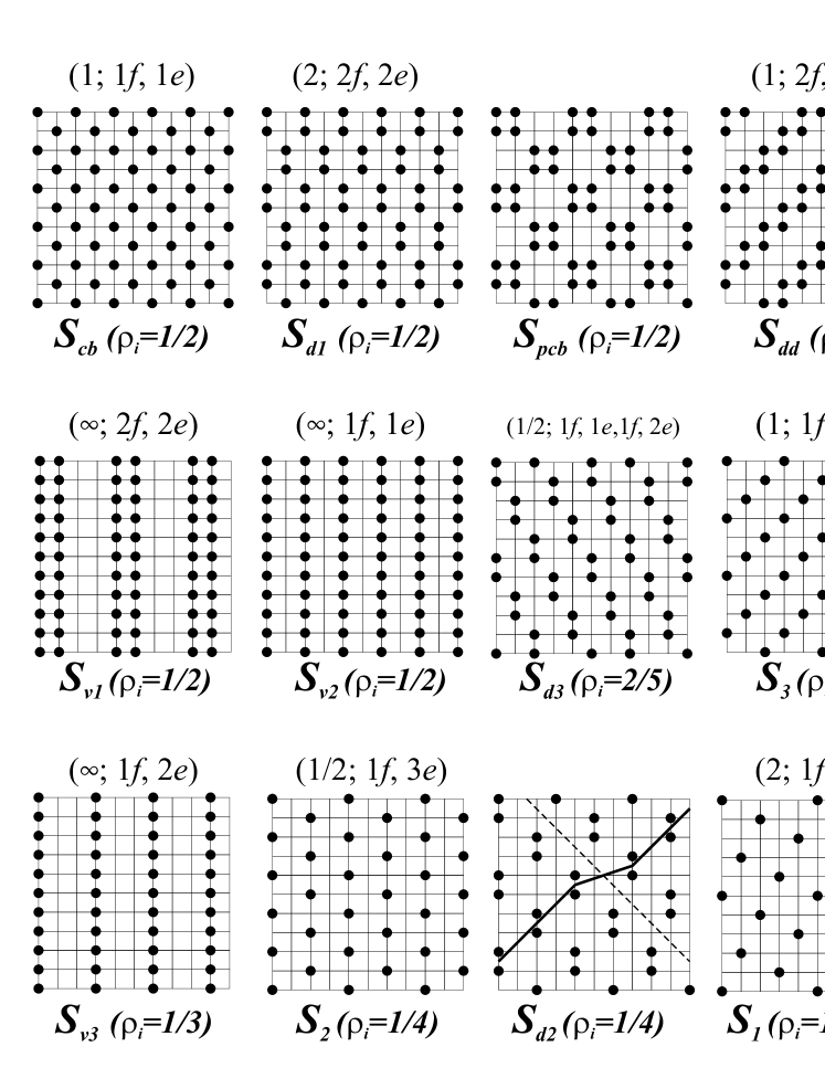
Figure 8: Representative configurations of the sets ${\mathcal{S}}_{D}$ of ground-state configurations. The remaining configurations of ${\mathcal{S}}_{D}$ can be obtained by applying the symmetries of $H_{0}$ to the displayed configurations. As a representative configuration of ${\mathcal{S}}_{d2}$, we show a configuration with one defect line (the dashed line). The continuous line is a guide for the eye. For more comments see the text.

That is, the remaining configurations of ${\mathcal{S}}_{D}$ can be obtained easily by applying the symmetries of $H_{0}$ to the displayed configurations. The domain ${\mathcal{S}}_{seg}$, having no representative in Fig. 8, consists of the two translation-invariant configurations $S_{+}$ and $S_{-}$, related by the hole-particle transformation.

Only in the domain ${\mathcal{S}}_{d2}$, which appears in the phase diagrams shown in Fig. 7, 7, that is off the hole-particle symmetry plain, the situation is not that simple. In ${\mathcal{S}}_{d2}$ one can distinguish two classes, ${\mathcal{S}}_{d2a}$ and ${\mathcal{S}}_{d2b}$, of periodic configurations with parallelogram elementary cells. A configuration in ${\mathcal{S}}_{d2a}$ consists of vertical (horizontal) dimers of filled sites that form a square lattice, where the sides of the elementary squares have the length $2\sqrt{2}$ and the slope $\pm 1$. In a configuration of ${\mathcal{S}}_{d2b}$, the elementary parallelograms formed by dimers have the sides of the length $2\sqrt{2}$ and the slope $\pm 1$, and the sides of the length $\sqrt{10}$ and the slope $\pm 1/3$. Two configurations, one from ${\mathcal{S}}_{d2a}$ and one from ${\mathcal{S}}_{d2b}$, having the same kind of dimers (vertical or horizontal), can be merged together along a “defect line” of the slope $\pm 1$ (dashed line in Fig. 8), as shown in Fig. 8, without increasing the energy. By introducing more defect lines one can construct many ground-state configurations whose number scales with the size of the lattice as $\exp{(const\sqrt{\Lambda})}$. While for a finite lattice all the configurations are periodic, many of them become aperiodic in the infinite volume limit.

As mentioned above, except ${\mathcal{S}}_{d2}$ all the other sets ${\mathcal{S}}_{D}$ contain exclusively periodic configurations. The set ${\mathcal{S}}_{pcb}$ (of plaquette-chessboard configurations) contains configurations built out of elementary plaquettes with filled sites, forming a square lattice according to the same rules as filled sites form a square lattice in the chessboard configurations from ${\mathcal{S}}_{cb}$. The remaining sets ${\mathcal{S}}_{D}$ consist of configurations that have a quasi-one-dimensional structure. That is, they are built out of completely filled and completely empty lattice lines of given slope. Such a configuration can be specified by the slope of the filled lattice lines of the representative configuration and the succession of filled (f) and empty (e) consecutive lattice lines in a period. For instance, the representative configuration of ${\mathcal{S}}_{d1}$ (see Fig. 8) is built out of filled lines with the slope $2$ and, in the period, two consecutive filled lines are followed by two consecutive empty lines, which is denoted $(2;2f,2e)$. Similar description of the remaining quasi-one-dimensional configurations is given in Fig. 8.

The coefficients $\{\alpha_{i}\}$ for which the fourth order potentials, $(H^{fermion}_{T})^{(4)}+K^{(4)}_{T}$ and $(H^{boson}_{T})^{(4)}+K^{(4)}_{T}$, become $m$-potentials are given in the tables collected in the Appendix.

Finally, a remark concerning ground-state configurations at the boundaries between the open domains ${\mathcal{S}}_{D}$ is in order. Let ${\mathcal{S}}_{D}$ and ${\mathcal{S}}_{D^{\prime}}$ be two domains of the considered phase diagram, sharing a boundary. At this boundary, the set of the minimizing $T$-plaquette configurations contains always the subset ${\mathcal{S}}_{TD}\cup{\mathcal{S}}_{TD^{\prime}}$, but it may contain also some additional $T$-plaquette configurations of minimal energy. Consequently, the set of the ground-state configurations at the boundary contains always the subset ${\mathcal{S}}_{D}\cup{\mathcal{S}}_{D^{\prime}}$ and typically a great many of other ground-state configurations, whose number grows indefinitely with the size of the lattice. In the considered diagrams, the only exception is the boundary between ${\mathcal{S}}_{seg}$ and ${\mathcal{S}}_{cb}$, where the set of the ground-state configurations amounts exactly to ${\mathcal{S}}_{seg}\cup{\mathcal{S}}_{cb}$.

4 Discussion of the phase diagrams and conclusions

We start with a few comments concerning the phase diagrams due to the fourth order effective interactions. In the fourth order effective interaction, the parameters $\omega$ and $\varepsilon$ control the strength of n.n. and n.n.n. interactions, respectively. The n.n. interaction is repulsive and favors the chessboard configurations if $\omega>9/2$, for fermions ($\omega>5/2$, for bosons). In the opposite case (attraction) it favors the $S_{+}$, $S_{-}$ configurations. In turn, the n.n.n. interaction is attractive if $\varepsilon>3$, for fermions ($\varepsilon>5$, for bosons), and then it reinforces the tendency towards chessboard and uniform, $S_{+}$, $S_{-}$, configurations. When it becomes repulsive, it frustrates the n.n. interaction: the more negative it is the larger $\omega$ is needed to stabilize the chessboard configurations and the smaller $\omega$ is needed to stabilize the $S_{+}$, $S_{-}$ configurations. Therefore, whatever the value of $\varepsilon$ is, there is a sufficiently large $\omega$ such that $(\varepsilon,\omega)\in{\mathcal{S}}_{cb}$ and a sufficiently small $\omega$ such that $(\varepsilon,\omega)\in{\mathcal{S}}_{seg}$.

Apparently, the fourth order phase diagrams in the cases of hoping fermions and hoping bosons are quite similar if we compare the geometry of the phase boundaries and the sets of ground states. The main difference is in the domain occupying the central position: in the case of fermions the ground-state configurations are diagonal-stripe configurations, ${\mathcal{S}}_{dd}$, while in the case of bosons this is the set ${\mathcal{S}}_{pcb}$ of plaquette-chessboard configurations. These two sets of configurations are ground-state configurations of the corresponding fourth-order effective interactions with the site, n.n., and n.n.n. terms dropped, which corresponds to the points $(9/2,3)\in{\mathcal{S}}_{dd}$ and $(5/2,5)\in{\mathcal{S}}_{pcb}$. This means that the fourth order phase diagrams can be looked upon as the result of perturbing an Ising-like Hamiltonian, that consists of pair interactions at distance of two lattice constants and plaquette interactions, by n.n. and n.n.n. interactions. More generally, it is easy to verify that the set of ground-state configurations of the Ising-like Hamiltonian,

$$\sum\limits_{\langle x,y\rangle_{3}}s_{x}s_{y}+\gamma\sum\limits_{P}s_{P},$$ (20)

amount to ${\mathcal{S}}_{dd}$ if $\gamma>0$, and to ${\mathcal{S}}_{pcb}$ if $\gamma<0$. These ground states are stable with respect to perturbations by n.n. and n.n.n. interactions, if the corresponding interaction constants are in a certain vicinity of zero. Otherwise, new sets of ground states, shown in Fig. 5 and Fig. 5 emerge.

The basic question to be answered, before discussing the phase diagrams due to the complete interaction, refers to the relation between these phase diagrams and the diagrams due to the truncated effective interactions, obtained in the previous section.

Firstly, we note, by inspection of the phase boundaries in Fig. 5 and Fig. 5, that the $T$-plaquette configurations $\{45,58\}$ are missing in the phase diagram corresponding to fermion mobile particles. In turn, the $T$-plaquette configurations $\{41,62\}$ are missing in the phase diagram corresponding to boson mobile particles. Consequently, the ground-state configurations of ${\mathcal{S}}_{pcb}$ cannot appear not only in the fourth order fermion phase diagram but also in the fermion phase diagram of the complete interaction. Similarly, the ground-state configurations of ${\mathcal{S}}_{dd}$ do not appear in boson phase diagrams.

Secondly, by adapting the arguments presented in [29, 27], we can demonstrate, see for instance [31], that if the remainder $R^{(4)}$ is taken into account, then there is a (sufficiently small) constant $t_{0}$ such that for $t<t_{0}$ the phase diagram looks the same as the phase diagram due to the effective interaction truncated at the fourth order, except some regions of width $O(t^{6})$, located along the boundaries between the domains, and except the domain ${\mathcal{S}}_{d2}$. For $t<t_{0}$ and each domain ${\mathcal{S}}_{D}$, ${\mathcal{S}}_{D}\neq{\mathcal{S}}_{d2}$, there is a nonempty two-dimensional open domain ${\mathcal{S}}_{D}^{\infty}$ that is contained in the domain ${\mathcal{S}}_{D}$ and such that in ${\mathcal{S}}_{D}^{\infty}$ the set of ground-state configurations coincides with ${\mathcal{S}}_{D}$.

Now, consider our systems for specified particle densities, $\rho_{e}=\rho_{i}=1/2$. According to the phase diagrams in the hole-particle symmetry plane ($\mu=\delta=0$), shown in Fig. 5 and Fig. 5, if $(\varepsilon,\omega)$ is in ${\mathcal{S}}_{seg}^{\infty}$, then the ground state is a phase-separated state, where ion configurations are mixtures of $S_{+}$ and $S_{-}$ configurations, called the segregated phase. Another phase-separated state, where the ion configurations are mixtures of $S_{+}$, $S_{-}$, $S_{cb}^{e}$, and $S_{cb}^{o}$ configurations, exists at a line that is a small ($O(t^{2})$) distortion of the boundary between the domains ${\mathcal{S}}_{seg}$ and ${\mathcal{S}}_{cb}$ [29]. In all the other domains ${\mathcal{S}}_{D}^{\infty}$ of these diagrams the ground-state phase exhibits a crystalline long-range order of ions.

By the properties of the fourth order phase diagrams, whatever the value of $\varepsilon$ is, there is a sufficiently large $\omega$ such that the systems are in the chessboard phase ($(\varepsilon,\omega)\in{\mathcal{S}}_{cb}^{\infty}$) and a sufficiently small $\omega$ such that the systems are in the segregated phase ($(\varepsilon,\omega)\in{\mathcal{S}}_{seg}^{\infty}$). In between, the systems undergo a series of phase transitions and visit various striped phases. Consider first unbiased systems ($\varepsilon=0$). Then, it follows from the phase diagram in Fig. 5, that the fermion system visits necessarily the diagonal striped phase, described by the configurations in ${\mathcal{S}}_{dd}$. In turn, the phase diagram in Fig. 5 implies that the boson system has to visit the dimerized-chessboard phase, described by the configurations in ${\mathcal{S}}_{d1}$, then the vertical/horizontal striped phase, described by the configurations in ${\mathcal{S}}_{v2}$, and after that a dimerized vertical/horizontal striped phase, described by the configurations in ${\mathcal{S}}_{v1}$. These scenarios are preserved, if $\varepsilon\in(-2+O(t^{2}),12-O(t^{2}))$ in the fermion case, and $\varepsilon\in(-\infty,1-O(t^{2}))$ in the boson case.

Note that the same sequence of transitions, as found in the unbiased boson system, can be realized by the fermion system if $\varepsilon$ is sufficiently small ($\varepsilon<-6-O(t^{2})$).

For somewhat larger values of $\varepsilon$, $\varepsilon\in(-6+O(t^{2}),-2-O(t^{2}))$, on its way from the chessboard phase to the segregated phase the fermion systems visits the dimerized chessboard phase, then the diagonal striped phase, and after that the dimerized vertical/horizontal striped phase. The vertical/horizontal striped phase is closer to the segregated phase than the diagonal striped phase. In case the both kinds of stripe phases (vertical/horizontal and diagonal) appear in a phase diagram, such a succession of striped phases is perhaps generic, see also [15, 32].

For sufficiently large $\varepsilon$, the tendency toward the chessboard and the uniform configurations is so strong that the both systems jump directly from the chessboard phase to the segregated phase.

Above, we have described the states of the considered systems for typical values of the control parameter $\omega$. Only in small intervals (whose width is of the order of $O(t^{2})$) of values of $\omega$, about the transition points of the diagrams in Fig. 5 and Fig. 5, the states of the systems remain undetermined.

For completeness we present also ground-state phase diagrams of the both systems off the hole-particle symmetry plane, for $\varepsilon=0$, see Fig. 7, 7. Away from the hole-particle symmetry plane new phases appear. In particular we find the phases described by the quasi-one-dimensional configurations ${\mathcal{S}}_{1}$, ${\mathcal{S}}_{2}$, and ${\mathcal{S}}_{3}$, well known from the studies of the phase diagram of the spinless Falicov–Kimball model [27]. In the boson phase diagram, Fig. 7, there appears the domain ${\mathcal{S}}_{d2}$ that is not amenable to the kind of arguments used in this paper.

5 Summary

In this paper, we address the problem of the stability of charge-stripe phases versus the phase separated state — the segregated phase, in strongly-interacting systems of fermions or hardcore bosons. There are numerous works devoted to this problem, where it is studied, by approximate methods, in the framework of relevant for experiments models. Unfortunately, due to tiny energy differences involved, it is difficult to settle this problem by means of approximate methods, which bias the calculated energies with hardly controllable errors of various nature. We have studied simple models, that by many physicists can be considered less realistic, but which, in return, are amenable to a rigorous analysis. Our models are described by extended Falicov–Kimball Hamiltonians, with hoping particles being spinless fermions or hardcore bosons. The ground-state phase diagrams of these models have been constructed rigorously in the regime of strong coupling and half-filling. In the both cases, of fermions and hardcore bosons, we have found transitions from a crystalline chessboard phase to the segregated phase via striped phases.

6 Appendix

In this section, at each point $p=(\omega,\varepsilon)$ we give the sets $\{\alpha_{i}(p)\}$ of the zero-potential coefficients $\alpha_{i}$ that we used to construct the four phase diagrams, presented in the previous section. Specifically, for each of the four phase diagrams we define a partition, called $\alpha$-partition, of the $(\omega,\varepsilon)$-plane (see the tables displayed below) into sets that differ, in general, from the domains ${\mathcal{S}}_{D}$. To each set of such a partition we assign a set $\{(a_{i},b_{i},c_{i})\}$ of triplets of rational numbers, such that the coefficients $\alpha_{i}(p)$ (with $p$ in the considered set) are affine functions of the form $a_{i}\omega+b_{i}\varepsilon+c_{i}$. We have not been able to find one set $\{(a_{i},b_{i},c_{i})\}$, that turns the fourth order potentials into $m$-potentials in the whole $(\omega,\varepsilon)$-plane. We have not also succeeded in assigning to each domain ${\mathcal{S}}_{D}$ an exactly one set $\{(a_{i},b_{i},c_{i})\}$. The same remarks apply to the $(\omega,\delta)$-plane.

Figure 9: The sets A, B, C, whose boundaries are marked with dashed lines, used in Table 1 to define the $\alpha$-partition of the fourth order phase diagram in the case of fermions and for $\delta=0$.The dashed-line segments are determined by their intersection points: ${\bf a}=(-1/2,-6)$, ${\bf b}=(-13/2,-10)$, ${\bf c}=(19/2,-6)$, ${\bf d}=(31/2,-10)$. The coordinates of the remaining points can be read from Fig. 5.

Figure 10: The sets A, B, C, whose boundaries are marked with dashed lines, used in Table 2 to define the $\alpha$-partition of the fourth order phase diagram in the case of hardcore bosons and for $\delta=0$. The dashed-line segments are determined by their intersection points: ${\bf a}=(1/2,4)$, ${\bf b}=(2,1)$, ${\bf c}=(-5/2,-2)$, ${\bf d}=(9/2,4)$, ${\bf e}=(3,1)$, ${\bf f}=(15/2,-2)$.

Table 1: The set of zero-potential coefficients $\{\alpha_{i}\}$ in the case of fermions and for $\delta=0$. In the first column the sets of the $\alpha$-partition are specified. For more comments see the text in Appendix.

	$\alpha_{1}$	$\alpha_{2}$	$\alpha_{3}$	$\alpha_{4}$	$\alpha_{5}$
A	$0$	$0$	$-\frac{\omega}{96}+\frac{3}{64}$	$0$	$-\frac{1}{48}$
${\mathcal{S}}_{dd}\cap$B	$0$	$0$	$-\frac{5\omega}{192}-\frac{\varepsilon}{64}-\frac{3}{128}$	$\frac{\omega}{32}+\frac{\varepsilon}{32}+\frac{9}{64}$	$\frac{\omega}{64}+\frac{\varepsilon}{64}+\frac{19}{384}$
${\mathcal{S}}_{v1}\cap$B	$0$	$0$	$\frac{\omega}{192}-\frac{\varepsilon}{64}+\frac{7}{128}$	$-\frac{\omega}{32}+\frac{\varepsilon}{32}-\frac{1}{64}$	$-\frac{\omega}{64}+\frac{\varepsilon}{64}-\frac{11}{384}$
${\mathcal{S}}_{v2}\cap$B	$0$	$0$	$-\frac{5\omega}{192}+\frac{\varepsilon}{64}+\frac{21}{128}$	$\frac{\omega}{32}-\frac{\varepsilon}{32}-\frac{15}{64}$	$\frac{\omega}{64}-\frac{\varepsilon}{64}-\frac{53}{384}$
${\mathcal{S}}_{dd}\cap$C	$0$	$0$	$-\frac{5\omega}{192}+\frac{\varepsilon}{64}+\frac{33}{128}$	$-\frac{\omega}{32}+\frac{\varepsilon}{32}+\frac{27}{64}$	$-\frac{\omega}{64}+\frac{\varepsilon}{64}+\frac{73}{384}$
${\mathcal{S}}_{v2}\cap$C	$0$	$0$	$-\frac{5\omega}{192}-\frac{\varepsilon}{64}+\frac{9}{128}$	$-\frac{\omega}{32}-\frac{\varepsilon}{32}+\frac{3}{64}$	$-\frac{\omega}{64}-\frac{\varepsilon}{64}+\frac{1}{384}$
${\mathcal{S}}_{d1}\cap$C	$0$	$0$	$\frac{\omega}{192}+\frac{\varepsilon}{64}-\frac{13}{128}$	$\frac{\omega}{32}+\frac{\varepsilon}{32}-\frac{19}{64}$	$\frac{\omega}{64}+\frac{\varepsilon}{64}-\frac{65}{384}$

Table 2: The set of zero-potential coefficients $\{\alpha_{i}\}$ in the case of hardcore bosons and for $\delta=0$. In the first column the sets of the $\alpha$-partition are specified. For more comments see the text in Appendix.

	$\alpha_{1}$	$\alpha_{2}$	$\alpha_{3}$	$\alpha_{4}$	$\alpha_{5}$
A	$0$	$0$	$-\frac{\omega}{96}+\frac{5}{192}$	$0$	$-\frac{1}{48}$
${\mathcal{S}}_{pcb}\cap$B	$0$	$0$	$-\frac{\omega}{24}-\frac{\varepsilon}{64}+\frac{23}{192}$	$\frac{\omega}{16}+\frac{7\varepsilon}{192}-\frac{37}{192}$	$\frac{\omega}{32}+\frac{5\varepsilon}{256}-\frac{91}{768}$
${\mathcal{S}}_{v1}\cap$B	$0$	$0$	$\frac{\omega}{192}-\frac{\varepsilon}{64}+\frac{37}{384}$	$-\frac{7\omega}{192}+\frac{7\varepsilon}{192}-\frac{55}{384}$	$-\frac{5\omega}{256}+\frac{5\varepsilon}{256}-\frac{143}{1536}$
${\mathcal{S}}_{v2}\cap$B	$0$	$0$	$-\frac{\omega}{24}+\frac{\varepsilon}{32}+\frac{7}{96}$	$\frac{\omega}{16}-\frac{\varepsilon}{16}-\frac{3}{32}$	$\frac{\omega}{32}-\frac{\varepsilon}{32}-\frac{13}{192}$
${\mathcal{S}}_{pcb}\cap$C	$0$	$0$	$-\frac{\omega}{24}+\frac{\varepsilon}{64}+\frac{17}{192}$	$-\frac{\omega}{16}+\frac{7\varepsilon}{192}+\frac{23}{192}$	$-\frac{\omega}{32}+\frac{5\varepsilon}{256}+\frac{29}{768}$
${\mathcal{S}}_{v2}\cap$C	$0$	$0$	$-\frac{\omega}{24}-\frac{\varepsilon}{32}+\frac{13}{96}$	$-\frac{\omega}{16}-\frac{\varepsilon}{16}+\frac{7}{32}$	$-\frac{\omega}{32}-\frac{\varepsilon}{32}+\frac{17}{192}$
${\mathcal{S}}_{d1}\cap$C	$0$	$0$	$\frac{\omega}{192}+\frac{\varepsilon}{64}-\frac{47}{384}$	$\frac{7\omega}{192}+\frac{7\varepsilon}{192}-\frac{125}{384}$	$\frac{5\omega}{256}+\frac{5\varepsilon}{256}-\frac{293}{1536}$

Figure 11: The sets A,B,…, whose boundaries are marked with dashed and continuous lines (the continuous lines are the boundaries of the phase diagram), used in Table 3 to define the $\alpha$-partition of the fourth order phase diagram in the case of fermions and for $\varepsilon=0$.

Figure 12: The sets A,B,…, whose boundaries are marked with dashed and continuous lines (the continuous lines are the boundaries of the phase diagram), used in Table 4 to define the $\alpha$-partition of the fourth order phase diagram in the case of hardcore bosons and for $\varepsilon=0$. The dashed-line segments are determined by their intersection points: ${\bf a}=(-5/2,-1)$, ${\bf b}=(3/2,-3)$, ${\bf c}=(7/2,-13/3)$, ${\bf d}=(9/2,-5)$, ${\bf e}=(6,-4)$, ${\bf f}=(29/4,-3)$.

Table 3: The set of zero-potential coefficients $\{\alpha_{i}\}$ in the case of fermions and for $\varepsilon=0$. In the first column the sets of the $\alpha$-partition are specified. For more comments see the text in Appendix.

	$\alpha_{1}$	$\alpha_{2}$	$\alpha_{3}$	$\alpha_{4}$	$\alpha_{5}$
${\mathcal{S}}_{-}\cap$D	$-\frac{201\delta}{3200}$	$-\frac{\delta}{8}$	$-\frac{\omega}{96}+\frac{\delta}{6400}+\frac{3}{64}$	$0$	$-\frac{1}{48}$
${\mathcal{S}}_{-}\cap$E	$\frac{\omega}{32}-\frac{\delta}{16}+\frac{3}{64}$	$-\frac{\delta}{8}$	$-\frac{\omega}{96}+\frac{3}{64}$	$0$	$-\frac{1}{48}$
${\mathcal{S}}_{-}\cap$F	$\frac{\omega}{48}-\frac{\delta}{16}+\frac{5}{96}$	$-\frac{\delta}{8}$	$\frac{1}{24}$	$0$	$-\frac{1}{48}$
${\mathcal{S}}_{1}\cap$G	$\frac{11\omega}{960}-\frac{9\delta}{160}+\frac{121}{1920}$	$-\frac{\delta}{8}$	$-\frac{7\omega}{5760}+\frac{\delta}{320}+\frac{403}{11520}$	$-\frac{\omega}{180}-\frac{\delta}{80}-\frac{11}{360}$	$-\frac{\omega}{144}+\frac{1}{288}$
${\mathcal{S}}_{1}\cap$H	$-\frac{3\omega}{160}-\frac{13\delta}{160}+\frac{11}{160}$	$\frac{\omega}{40}-\frac{\delta}{10}+\frac{1}{80}$	$-\frac{13\omega}{960}-\frac{\delta}{320}+\frac{17}{320}$	$-\frac{\omega}{40}-\frac{\delta}{40}-\frac{1}{80}$	$-\frac{1}{48}$
${\mathcal{S}}_{2}\cap$I	$-\frac{9\delta}{128}+\frac{21}{256}$	$-\frac{5\delta}{64}+\frac{9}{128}$	$-\frac{\omega}{96}+\frac{\delta}{128}+\frac{19}{256}$	$-\frac{3\delta}{128}-\frac{17}{256}$	$\frac{\omega}{512}-\frac{13}{3072}$
${\mathcal{S}}_{2}\cap$J	$\frac{\omega}{128}-\frac{7\delta}{128}+\frac{3}{64}$	$-\frac{\omega}{64}-\frac{9\delta}{64}+\frac{3}{32}$	$-\frac{\omega}{96}+\frac{1}{16}$	$\frac{\omega}{128}+\frac{\delta}{128}-\frac{5}{64}$	$\frac{\omega}{128}+\frac{\delta}{128}-\frac{7}{192}$
${\mathcal{S}}_{3}$	$-\frac{7\omega}{384}-\frac{17\delta}{192}+\frac{49}{256}$	$-\frac{\delta}{8}$	$-\frac{29\omega}{2304}-\frac{7\delta}{1152}+\frac{107}{1536}$	$\frac{\omega}{144}+\frac{\delta}{144}-\frac{7}{96}$	$-\frac{\omega}{144}-\frac{\delta}{144}+\frac{5}{96}$
${\mathcal{S}}_{cb}$	$-\frac{359\delta}{5728}$	$-\frac{\delta}{8}$	$-\frac{173\omega}{17184}+\frac{3\delta}{11456}+\frac{495}{11456}$	$0$	$-\frac{1}{48}$
${\mathcal{S}}_{dd}\cap$A	$-\frac{\delta}{8}$	$-\frac{\delta}{8}$	$-\frac{\omega}{96}+\frac{\delta}{96}+\frac{3}{64}$	$\frac{\delta}{48}$	$-\frac{\delta}{48}-\frac{1}{48}$
${\mathcal{S}}_{dd}\cap$B	$-\frac{\delta}{8}$	$-\frac{\delta}{8}$	$\frac{\delta}{96}+\frac{1}{24}$	$\frac{\delta}{48}$	$-\frac{\delta}{48}-\frac{1}{48}$
${\mathcal{S}}_{dd}\cap$C	$-\frac{\delta}{8}$	$-\frac{\delta}{8}$	$-\frac{\omega}{96}-\frac{\delta}{96}+\frac{3}{64}$	$\frac{\delta}{48}$	$-\frac{\delta}{48}-\frac{1}{48}$

Table 4: The set of zero-potential coefficients $\{\alpha_{i}\}$ in the case of hardcore bosons and for $\varepsilon=0$. In the first column the sets of the $\alpha$-partition are specified. The cases, where the set ${\mathcal{S}}_{D|T}$ is a proper subset of ${\mathcal{S}}_{TD}(p)$ are marked by the asterisk. For more comments see the text in Appendix.

	$\alpha_{1}$	$\alpha_{2}$	$\alpha_{3}$	$\alpha_{4}$	$\alpha_{5}$
${\mathcal{S}}_{-}\cap$I	$-\frac{\delta}{16}$	$-\frac{\delta}{8}$	$-\frac{\omega}{96}-\frac{1}{192}$	$0$	$-\frac{1}{48}$
${\mathcal{S}}_{-}\cap$J	$\frac{\omega}{32}-\frac{\delta}{16}+\frac{9}{64}$	$-\frac{\delta}{8}$	$\frac{7\omega}{192}+\frac{3\delta}{32}+\frac{91}{384}$	$-\frac{3\omega}{64}-\frac{3\delta}{32}-\frac{27}{128}$	$-\frac{1}{48}$
${\mathcal{S}}_{-}\cap$K	$-\frac{3\omega}{128}-\frac{\delta}{16}-\frac{7}{256}$	$\frac{3\omega}{64}-\frac{\delta}{8}+\frac{23}{128}$	$\frac{\omega}{48}+\frac{\delta}{16}+\frac{19}{96}$	$-\frac{\omega}{32}-\frac{3\delta}{64}-\frac{21}{128}$	$-\frac{15\omega}{512}-\frac{7\delta}{256}-\frac{331}{3072}$
${\mathcal{S}}_{-}\cap$L	$\frac{\omega}{16}-\frac{\delta}{16}-\frac{5}{32}$	$-\frac{\omega}{8}-\frac{\delta}{8}+\frac{7}{16}$	$\frac{11\omega}{384}+\frac{3\delta}{32}+\frac{203}{768}$	$\frac{21\omega}{128}+\frac{5\delta}{32}+\frac{13}{256}$	$-\frac{41\omega}{512}-\frac{19\delta}{128}-\frac{1027}{3072}$
${\mathcal{S}}_{-}\cap$M	$-\frac{\delta}{16}+\frac{1}{16}$	$-\frac{\omega}{32}-\frac{5\delta}{32}-\frac{1}{64}$	$-\frac{23\omega}{768}-\frac{5\delta}{256}+\frac{25}{1536}$	$\frac{7\omega}{128}+\frac{7\delta}{128}+\frac{7}{256}$	$-\frac{\omega}{128}-\frac{\delta}{128}-\frac{19}{768}$
${\mathcal{S}}_{1}\cap$S	$-\frac{9\omega}{160}-\frac{11\delta}{40}-\frac{189}{320}$	$\frac{\omega}{20}+\frac{\delta}{20}+\frac{21}{40}$	$-\frac{5\omega}{192}-\frac{\delta}{16}-\frac{65}{384}$	$-\frac{3\omega}{80}-\frac{\delta}{10}-\frac{43}{160}$	$-\frac{\omega}{80}-\frac{3\delta}{40}-\frac{133}{480}$
${\mathcal{S}}_{1}\cap$T	$-\frac{\omega}{40}-\frac{7\delta}{80}+\frac{1}{20}$	$\frac{\omega}{40}-\frac{\delta}{10}+\frac{1}{80}$	$-\frac{\omega}{60}-\frac{\delta}{160}+\frac{11}{480}$	$-\frac{\omega}{40}-\frac{\delta}{40}-\frac{1}{80}$	$-\frac{1}{48}$
${\mathcal{S}}_{3}\cap$P	$-\frac{\omega}{192}-\frac{\delta}{12}-\frac{5}{384}$	$-\frac{\delta}{8}$	$-\frac{\omega}{288}-\frac{5\delta}{144}-\frac{83}{576}$	$\frac{\omega}{192}-\frac{\delta}{24}-\frac{67}{384}$	$-\frac{\omega}{288}-\frac{\delta}{72}-\frac{17}{576}$
${\mathcal{S}}_{3}\cap$Q	$\frac{25\omega}{192}-\frac{\delta}{6}-\frac{475}{384}$	$-\frac{\omega}{8}-\frac{\delta}{16}+\frac{35}{32}$	$\frac{3\omega}{128}-\frac{7\delta}{192}-\frac{269}{768}$	$\frac{\omega}{16}-\frac{\delta}{32}-\frac{37}{64}$	$\frac{5\omega}{96}-\frac{\delta}{24}-\frac{33}{64}$
${\mathcal{S}}_{3}\cap$R	$-\frac{\delta}{16}$	$-\frac{\omega}{72}-\frac{5\delta}{36}+\frac{13}{144}$	$-\frac{\omega}{144}+\frac{\delta}{288}+\frac{1}{288}$	$\frac{\omega}{72}+\frac{\delta}{72}-\frac{13}{144}$	$-\frac{1}{48}$
${\mathcal{S}}_{cb}$	$-\frac{\delta}{16}$	$-\frac{\delta}{8}$	$-\frac{\omega}{96}+\frac{5}{192}$	$0$	$-\frac{1}{48}$
${\mathcal{S}}_{v1}$	$-\frac{3\delta}{16}$	$-\frac{\delta}{8}$	$\frac{\omega}{192}+\frac{37}{384}$	$-\frac{\omega}{32}-\frac{\delta}{16}-\frac{9}{64}$	$-\frac{\omega}{64}-\frac{\delta}{8}-\frac{35}{384}$
${\mathcal{S}}_{v2}\cap$A	$-\frac{\delta}{32}$	$-\frac{3\delta}{16}$	$-\frac{\omega}{32}-\frac{\delta}{96}+\frac{5}{64}$	$-\frac{1}{8}$	$-\frac{1}{12}$
${\mathcal{S}}_{v2}\cap$B ∗	$\frac{\omega}{32}-\frac{\delta}{16}-\frac{11}{64}$	$-\frac{\omega}{16}-\frac{\delta}{8}+\frac{11}{32}$	$-\frac{\omega}{24}+\frac{13}{96}$	$-\frac{1}{8}$	$-\frac{1}{12}$
${\mathcal{S}}_{v3}$	$-\frac{\omega}{192}-\frac{\delta}{24}-\frac{1}{384}$	$-\frac{\omega}{32}-\frac{\delta}{4}-\frac{1}{64}$	$-\frac{7\omega}{192}-\frac{\delta}{48}+\frac{29}{384}$	$-\frac{\omega}{96}-\frac{\delta}{48}-\frac{25}{192}$	$-\frac{1}{12}$
${\mathcal{S}}_{d1}\cap$C	$-\frac{\delta}{16}$	$-\frac{\delta}{8}$	$\frac{\omega}{192}-\frac{47}{384}$	$\frac{3\omega}{64}-\frac{49}{128}$	$\frac{\omega}{32}-\frac{49}{192}$
${\mathcal{S}}_{d1}\cap$D	$-\frac{\delta}{16}$	$-\frac{\delta}{8}$	$\frac{\omega}{192}-\frac{47}{384}$	$\frac{\omega}{64}-\frac{19}{128}$	$-\frac{1}{48}$
${\mathcal{S}}_{d2}\cap$N	$\frac{\omega}{64}-\frac{\delta}{8}-\frac{31}{128}$	$-\frac{5\omega}{64}-\frac{\delta}{16}+\frac{67}{128}$	$-\frac{\omega}{24}+\frac{13}{96}$	$-\frac{\delta}{16}-\frac{1}{4}$	$\frac{\omega}{128}-\frac{\delta}{32}-\frac{133}{768}$
${\mathcal{S}}_{d2}\cap$O	$-\frac{3\omega}{32}-\frac{\delta}{8}+\frac{9}{64}$	$\frac{5\omega}{64}-\frac{\delta}{16}-\frac{3}{128}$	$-\frac{\omega}{24}+\frac{13}{96}$	$-\frac{3\omega}{64}-\frac{\delta}{16}-\frac{11}{128}$	$-\frac{3\omega}{128}-\frac{\delta}{32}-\frac{49}{768}$
${\mathcal{S}}_{d3}\cap$E ∗	$\frac{\omega}{32}-\frac{\delta}{16}-\frac{11}{64}$	$-\frac{\omega}{20}-\frac{3\delta}{20}+\frac{1}{4}$	$-\frac{\omega}{60}-\frac{\delta}{20}-\frac{5}{96}$	$\frac{\omega}{32}-\frac{\delta}{16}-\frac{23}{64}$	$\frac{3\omega}{160}-\frac{3\delta}{80}-\frac{43}{192}$
${\mathcal{S}}_{d3}\cap$F ∗	$-\frac{\delta}{16}$	$-\frac{3\omega}{160}-\frac{3\delta}{20}+\frac{5}{64}$	$-\frac{31\omega}{960}-\frac{\delta}{20}+\frac{13}{384}$	$-\frac{\delta}{16}-\frac{3}{16}$	$\frac{\omega}{320}-\frac{3\delta}{80}-\frac{53}{384}$
${\mathcal{S}}_{d3}\cap$G ∗	$\frac{3\omega}{64}+\frac{\delta}{16}+\frac{3}{128}$	$-\frac{\omega}{16}-\frac{\delta}{4}+\frac{3}{32}$	$-\frac{\omega}{240}+\frac{\delta}{20}+\frac{5}{48}$	$\frac{3\omega}{64}+\frac{\delta}{16}-\frac{21}{128}$	$\frac{9\omega}{320}+\frac{3\delta}{80}-\frac{41}{384}$
${\mathcal{S}}_{d3}\cap$H ∗	$\frac{\omega}{64}+\frac{\delta}{16}+\frac{25}{128}$	$-\frac{\omega}{32}-\frac{\delta}{4}-\frac{5}{64}$	$-\frac{19\omega}{960}+\frac{\delta}{20}+\frac{73}{384}$	$\frac{\omega}{64}+\frac{\delta}{16}+\frac{1}{128}$	$\frac{\omega}{80}+\frac{3\delta}{80}-\frac{1}{48}$

References

• [1] J.M. Tranquada, D.J. Buttrey, V. Sachan, and J.E. Lorenzo, Simultaneous Ordering of Holes and Spins in $La_{2}NiO_{4.125}$, Phys. Rev. Lett. 73, 1003 (1994)
• [2] J.M. Tranquada, B.J. Sternlieb, J.D. Axe, Y. Nakamura, and S. Uchida, Evidence for stripe correlations of spins and holes in copper oxide superconductors, Nature (London) 375, 561 (1995)
• [3] K. Kern, H. Niehus, A. Schatz, P. Zeppenfeld, J. Goerge, and G. Comsa, Long-Range Spatial Self-Organization in the Adsorbate-Induced Restructuring of Surfaces: Cu$\{110\}-(2\times 1)$O, Phys. Rev. Lett. 67, 855 (1991)
• [4] K. Sasaki, Lattice gas model for striped structures of adatom rows on surfaces, Surf. Sci. 318, L1230 (1994)
• [5] G. Malescio and G. Pellicane, Stripe phases from isotropic repulsive interactions, Nature Materials 2, 97 (2003)
• [6] D. Poilblanc and T.M. Rice, Charged solitons in the Hartree-Fock approximation to the large-$U$ Habbard model, Phys. Rev. B 39, 9749 (1989); K. Machida, Magnetism in $La_{2}CuO_{4}$ based compounds, Physica C 158, 192 (1989)
• [7] J. Zaanen and O. Gunnarsson, Charged magnetic domain lines and the magnetism of high-$T_{c}$ oxides, Phys. Rev. B 40, 7391 (1989); M. Kato, K. Machida, H. Nakanishi, and M. Fujita, Soliton lattice modulation of incommensurate spin density wave in two dimensional Hubbard model — a mean field study, J. Phys. Soc. Jpn., 59, 1047 (1990)
• [8] A.M. Oleś, Stripe phases in high-temperature superconductors, Acta Physica Polonica B 31, 2963 (2000)
• [9] S.R. White and D.J. Scalapino, Density Matrix Renormalization Group Study of the Striped Phase in the 2D $t$ $J$ Model, Phys. Rev. Lett. 80, 1272 (1998)
• [10] S.R. White and D.J. Scalapino, Energetics of Domain Walls in the 2D $t$ $J$ Model, Phys. Rev. Lett. 81, 3227 (1998)
• [11] V.J. Emery, S.A. Kivelson, and J.M. Tranquada, Stripe phases in high-temperature superconductors, Proc. Natl. Acad. Sci. USA 96, 8814 (1999)
• [12] N.G. Zhang and C.L. Henley, Stripes and holes in a two-dimensional model of spinless fermions or hardcore bosons, Phys. Rev. B 68, 014506 (2003)
• [13] A.W. Sandvik, S. Daul, R.R.P. Singh, and D.J. Scalapino, Striped Phase in a Quantum $XY$ Model with Ring Exchange, Phys. Rev. Lett. 89, 247201 (2002)
• [14] C. Buhler, S. Yunoki, and A. Moreo, Magnetic Domains and Stripes in a Spin-Fermion Model for Cuprates, Phys. Rev. Lett. 84, 2690 (2000)
• [15] R. Lemański, J.K. Freericks, and G. Banach, Stripe Phases in the Two-Dimensional Falicov–Kimball Model, Phys. Rev. Lett. 89, 196403 (2002)
• [16] R. Lemański, J.K. Freericks, and G. Banach, Charge Stripes due to Electron Correlations in the Two-Dimensional Spinless Falicov–Kimball Model, J. Stat. Phys. 116, 699 (2004)
• [17] C.L. Henley and N.G. Zhang, Spinless fermions and charged stripes at the strong-coupling limit, Phys. Rev. B 63, 233107 (2001)
• [18] J.K.Freericks, E.H. Lieb, and D. Ueltschi, Phase separation due to quantum mechanical correlations, Phys. Rev. Lett. 88, 106401 (2002).
• [19] J.K.Freericks, E.H. Lieb, and D. Ueltschi, Segregation in the Falicov–Kimball model, Commun. Math. Phys. 227, 243 (2002).
• [20] L.M. Falicov and J.C. Kimball, Simple model for semiconductor-metal transitions: $SmB_{6}$ and transition-metal oxides, Phys. Rev. Lett. 22, 997 (1969).
• [21] U. Brandt, R. Schmidt, Exact results for the distribution of the $f$-level ground state occupation in the spinless Falicov–Kimball model, Z. Phys. B 63, 45 (1986).
• [22] T. Kennedy and E. H. Lieb, An itinerant electron model with crystalline or magnetic long range order, Physica A 138, 320 (1986).
• [23] C. Gruber and N. Macris, The Falicov–Kimball model: a review of exact results and extensions, Helv. Phys. Acta 69, 850 (1996).
• [24] J. Jȩdrzejewski and R. Lemański, Falicov–Kimball models of collective phenomena in solids (a concise guide), Acta Phys. Pol. B 32, 3243 (2001).
• [25] C. Gruber, J. Jȩdrzejewski and P. Lemberger, Ground states of the spinless Falicov–Kimball model. II, J. Stat. Phys. 66, 913 (1992).
• [26] A. Messager and S. Miracle-Solé, Low temperature states in the Falicov–Kimball model, Rev. Math. Phys. 8, 271 (1996).
• [27] C. Gruber, N. Macris, A. Messager and D. Ueltschi, Ground states and flux configurations of the two-dimensional Falicov–Kimball model, J. Stat. Phys. 86, 57 (1997).
• [28] J. Slawny, Low-temperature properties of classical lattice systems: phase transitions and phase diagrams, In: Phase Transitions and Critical Phenomena vol. 11, C. Domb and J. Lebowitz, eds (Academic Press, London/New York 1985).
• [29] T. Kennedy, Some rigorous results on the ground states of the Falicov–Kimball model, Rev. Math. Phys. 6, 901 (1994).
• [30] T. Kennedy, Phase separation in the neutral Falicov–Kimball model, J. Stat. Phys. 91, 829 (1998)
• [31] V. Derzhko and J. Jȩdrzejewski, From phase separation to long-range order in a system of interacting electrons, Physica A 328, 449 (2003)
• [32] C. Morais Smith, Yu.A. Dimashko, N. Hasselmann, and A.O. Caldeira, Dynamics of stripes in doped antiferromagnets, Phys. Rev. B 58, 453 (1998)