Absorption in atomic wires

Abstract

The transfer matrix formalism is implemented in the form of the multiple collision technique to account for dissipative transmission processes by using complex potentials in several models of atomic chains. The absorption term is rigorously treated to recover unitarity for the non-hermitian hamiltonians. In contrast to other models of parametrized scatterers we assemble explicit potentials profiles in the form of delta arrays, Pöschl-Teller holes and complex Scarf potentials. The techniques developed provide analytical expressions for the scattering and absorption probabilities of arbitrarily long wires. The approach presented is suitable for modelling molecular aggregate potentials and also supports new models of continuous disordered systems. The results obtained also suggest the possibility of using these complex potentials within disordered wires to study the loss of coherence in the electronic localization regime due to phase-breaking inelastic processes.

I Introduction

The inelastic scattering processes occurring in mesoscopic samples as a consequence of a finite non-zero temperature can noticeably change the coherent transport fingerprints of these structures. The worsening of electronic transmission due to such effects is expected but in some situations the competition between the phase-breaking mechanisms and the quantum coherent interferences can improve conductance in certain energetic regimes. This is the case, for example, of disordered structures. This fact has attracted much attention in the study and modelling of dissipative transport in one-dimensional structures. Interest is also prompted by experiments currently being carried out on real atomic chains vieira .

A model of parametrized scatterers coupled through additional side channels to electron reservoirs incorporating inelastic events was initially proposed by Büttiker butti , and much work has been done along this line bundle . On the other hand, inelastic processes can be modelled by small absorptions which in turn can be described by extending the nature of the quantum potentials to the complex domain. The main purpose of this work is to include absorptive processes by performing these complex extensions on previous quantum wire models developed by the authors aro and also on other atomic potentials.

The use of complex site energies and frequencies has already been considered in the study of electronic conductivity through one-dimensional chains kramer ; pataki , but non-hermitian hamiltonians have also been used to account for a large variety of phenomena, ranging from wave transport in absorbing media waves , violation of the single parameter scaling in one-dimensional absorbing systems deych , appearance of exceptional points in scattering theory epscatt and quantum chaology epcaos , description of vortex delocalization in superconductors with a transverse Meissner effect nelson and more phenomenologically with nuclear optical potentials. Special mention is required for the framework of $\mathcal{PT}$-symmetry pts , where it is possible to consider periodic wires under complex potentials showing real band spectra ptcer ; ptperio . There is nothing wrong in principle with the use of non-hermitian hamiltonians as long as their properties are controlled by a sufficient knowledge of the full spectrum. Indeed, renormalization group calculations have been carried out giving rise to imaginary couplings as a result of quantum dressing of the classical real potentials renorma .

An interesting modern review on absorption in quantum mechanics has appeared recently report and we address the interested reader to this publication and references therein.

The paper is organized as follows. In Section II we briefly review the multiple collision technique based on the transfer matrix method, and in Section III we show how unitarity can be easily restored in the presence of absorption and how the general unitarity condition can be generalized accordingly. We then turn our attention to arrays of delta potentials and calculate and draw the scattering and absorption probabilities in Section IV. In Section V, the Pöschl-Teller potential is used to build atomic chains, and its complex extension the complex Scarf potential is fully developed in Section VI. The analytical scattering probabilities are shown for a variety of composite potential profiles and the effect of the imaginary parts on the transmission is analyzed. The calculations concerning exact wave functions and analytical conditions are offered in two appendices. The paper ends with several concluding remarks.

II The multiple collision technique

The time-independent scattering process in one dimension can be described using the well known continuous transfer matrix method harrison ,

$$\begin{pmatrix}A_{R}\\ B_{R}\end{pmatrix}=\begin{pmatrix}M_{11}&M_{12}\\ M_{21}&M_{22}\end{pmatrix}\begin{pmatrix}A_{L}\\ B_{L}\end{pmatrix}$$ (1)

where $A_{L},B_{L}$$(A_{R},B_{R})$ mean the amplitudes of the asymptotic travelling plane waves $e^{ikx},e^{-ikx}$ at the left (right) side of the potential. Whatever the nature of the potential is, real or complex, the transmission matrix always verifies $\det\mathbf{M}=1$ as a consequence of the constant Wronskian of the solutions of the Schrödinger equation. The transmission and reflection amplitudes then read,

$$t=\frac{1}{M_{22}};\quad r^{L}=-\frac{M_{21}}{M_{22}};\quad r^{R}=\frac{M_{12}}{M_{22}}$$ (2)

where the superscripts $L,R$ stand for left and right incidence. The insensitivity of the transmission amplitude to the incidence direction is a universal property that holds for all kind of potentials. However, the reflectivity, although symmetric for real potentials, changes with the incidence side for a complex one unless it is symmetric zafarpra . The effect of a composition of $n$ different potentials can then be considered as the product of their transmission matrices,

$$\mathbb{M}=\mathbf{M}_{n}\ldots\mathbf{M}_{2}\mathbf{M}_{1}.$$ (3)

The transmission matrix formalism is an important tool for the numerical treatment of different problems. An intuitive and general interpretation of the composition procedure can be given in the following form. Consider two potentials $V_{1}(x),V_{2}(x)$ characterized by the scattering amplitudes $t_{1},r^{L}_{1},r^{R}_{1},t_{2},r^{L}_{2},r^{R}_{2}$ and joined at a certain point. Then, the scattering amplitudes of the composite potential can be obtained by considering the coherence sum of all the multiple reflection processes that might occur at the connection region,

$$t \equiv t_{1}\left\{\sum_{n=0}^{\infty}(r^{L}_{2}r^{R}_{1})^{n}\right\}t_{2}=\frac{t_{1}t_{2}}{1-r^{L}_{2}r^{R}_{1}}$$ (4a)

$$r^{L} \equiv r^{L}_{1}+t_{1}r^{L}_{2}\left\{\sum_{n=0}^{\infty}(r^{L}_{2}r^{R}_{1})^{n}\right\}t_{1}=r^{L}_{1}+\frac{r^{L}_{2}t_{1}^{2}}{1-r^{L}_{2}r^{R}_{1}}$$ (4b)

$$r^{R} \equiv r^{R}_{2}+t_{2}r^{R}_{1}\left\{\sum_{n=0}^{\infty}(r^{L}_{2}r^{R}_{1})^{n}\right\}t_{2}=r^{R}_{2}+\frac{r^{R}_{1}t_{2}^{2}}{1-r^{L}_{2}r^{R}_{1}}.$$ (4c)

Replacing the scattering amplitudes with the elements of the corresponding transmission matrices $\mathbf{M}_{1},\mathbf{M}_{2}$, one can trivially check that in fact these last formulae are the equations of the product $\mathbf{M}_{2}\mathbf{M}_{1}$. Thus, the composition rules given by (4) are not restricted to the convergence interval of the series $\sum_{n=0}^{\infty}(r^{L}_{2}r^{R}_{1})^{n}$. They provide an explicit relation of the global scattering amplitudes in terms of the individual former ones and can be easily used recurrently for numerical purposes. This composition technique was first derived for a potential barrier beam and has been used for designing absorbing potentials palao .

III The Schrödinger equation for a complex potential

Let us consider a one-dimensional complex potential of finite support $V(x)=V_{r}(x)+iV_{i}(x)$ ($V(\pm\infty)=0$). For the stationary scattering states, the density of the current flux is proportional to the imaginary part of the potential

$$\frac{dJ}{dx}=\frac{2}{\hbar}V_{i}(x)|\Psi(x)|^{2}$$ (5)

where $J(x)$ is defined as,

$$J(x)=\frac{\hbar}{2mi}\left(\Psi^{*}(x)\frac{d\Psi(x)}{dx}-\Psi(x)\frac{d\Psi^{*}(x)}{dx}\right).$$ (6)

Therefore, in the presence of a non-vanishing $V_{i}(x)$ the unitarity relation regarding the transmission and reflection probabilities $T(E)+R(E)=1$ is no longer valid. One can still recover a pseudounitarity relation by defining a quantity that accounts for the loss of flux in the scattering process. Dealing with the asymptotic state $\Psi^{L}_{k}(-\infty)=e^{ikx}+r^{L}(k)e^{-ikx}$, $\Psi^{L}_{k}(+\infty)=t(k)e^{ikx}$, one can write the asymptotic values of the flux as,

$$J_{-\infty} =\frac{\hbar k}{m}\left(1-R^{L}(k)\right)$$ (7)

$$J_{\infty} =\frac{\hbar k}{m}T(k)$$ (8)

yielding the relation,

$$T(k)+R^{L}(k)+\frac{m}{\hbar k}\left(J_{-\infty}-J_{\infty}\right)=1.$$ (9)

This latter equation remains the same for the right incidence case (with $R^{R}(k)$) when the asymptotic state takes the form $\Psi^{R}_{k}(-\infty)=t(k)e^{-ikx}$, $\Psi^{R}_{k}(+\infty)=e^{-ikx}+r^{R}(k)e^{ikx}$.

Using eq. (5) the flux term reads,

$$A^{L,R}(k) \equiv-\frac{2m}{\hbar^{2}k}\int_{-\infty}^{\infty}V_{i}(x)|\Psi^{L,R}_{k}(x)|^{2}dx$$

$$=1-R^{L,R}(k)-T(k),$$ (10)

and it is usually understood as the probability of absorption zafarpra . But $A(k)$ must be a positive defined quantity in order to be strictly considered as a probability and this is not ensured by the definition (unless $V_{i}(x)<0\;\forall\,x$). The sign of $A(k)$ depends on both the changes in sign of the imaginary part of the potential and the spatial distribution of the state. Although a negative value for $A(k)$ could be viewed as emission (because it means a gain in the flux current) it also leads the transmitivity and the reflectivity to attain anomalous values $T(k)>1,R(k)>1$, which are difficult to interpret. Let us also note that the integral representation of the absorption term is useless for practical purposes because to build the correct expression of the state $\Psi^{L,R}_{k}(x)$ one needs to impose the given asymptotic forms to the general solution of the Schrödinger equation, therefore obtaining the scattering amplitudes, so one cannot calculate the absorption probability without knowing $R(k)$ and $T(k)$.

IV Scattering of a chain of delta potentials

Let us consider a potential constituted by a finite array of Dirac delta distributions, each one with its own coupling $\alpha_{i}$ and equally spaced at a distance $a$. This is probably the simplest one-dimensional model imaginable, but in spite of its apparently simplicity it supports an unexpected physical richness. It has been successfully used to model band structure in a periodic quantum wire aro and has proved its usefulness when considering uncorrelated and correlated disorder structures aro ; adame , showing interesting effects such as the fractality of the density of states and the different localization regimes for the electronic states.

The global potential will be characterized by the arranged sequence of the parameters $(a/a_{i})$, where $a_{i}=\frac{\hbar^{2}}{m\alpha_{i}}$ means the “effective range” of the $i$th delta, in the order they appear from left to right. The transmission matrix for a delta potential preceded by a zero potential zone of length $a$ reads,

$$\mathbf{M}_{j}(k)=\begin{pmatrix}\left(1-\frac{i}{ka_{j}}\right)e^{ika}&-\frac{i}{ka_{j}}e^{-ika}\\ \frac{i}{ka_{j}}e^{ika}&\left(1+\frac{i}{ka_{j}}\right)e^{-ika}\end{pmatrix}.$$ (11)

Considering a chain of $N$ different deltas and applying the composition rules to this type of matrices one finds that it is possible to write a closed expression for the scattering amplitudes. They are given by,

$$t(k;a_{1},\ldots,a_{N}) =\frac{e^{iNka}}{f(k;a_{1},\ldots,a_{N})}$$ (12a)

$$r^{L}(k;a_{1},\ldots,a_{N}) =-\frac{g(k;a_{1},\ldots,a_{N})}{f(k;a_{1},\ldots,a_{N})}$$ (12b)

with the definitions

$$f(k;a_{1},\ldots,a_{N}) =1+\frac{i}{ka}\sum_{j=1}^{N}\left(\frac{a}{a_{j}}\right)+\sum_{j=2}^{N}\left(\frac{i}{ka}\right)^{j}\left\{\sum_{\sigma}\left[\left(\frac{a}{a_{\sigma_{1}}}\right)\left(\frac{a}{a_{\sigma_{2}}}\right)\ldots\left(\frac{a}{a_{\sigma_{j}}}\right)\prod_{r=1}^{j-1}\left(1-e^{2ika(\sigma_{r+1}-\sigma_{r})}\right)\right]\right\}$$ (13a)

$$g(k;a_{1},\ldots,a_{N}) =\frac{i}{ka}\sum_{j=1}^{N}e^{2ikaj}\left(\frac{a}{a_{j}}\right)+\sum_{j=2}^{N}\left(\frac{i}{ka}\right)^{j}\left\{\sum_{\sigma}\left[e^{2ika\sigma_{1}}\left(\frac{a}{a_{\sigma_{1}}}\right)\ldots\left(\frac{a}{a_{\sigma_{j}}}\right)\prod_{r=1}^{j-1}\left(1-e^{2ika(\sigma_{r+1}-\sigma_{r})}\right)\right]\right\}$$ (13b)

where for each $j$ the $\sum_{\sigma}$ means we are summing over the $\binom{N}{j}$ combinations of size $j$ from the set $\{1,2,\ldots,N\}$ $\sigma=\{\sigma_{1},\sigma_{2},\ldots,\sigma_{j}\}$ with $\sigma_{1}<\sigma_{2}<\ldots<\sigma_{j}$. The $r^{R}$ amplitude up to a phase is obtained from $r^{L}$ for the reverse chain. These latter formulae resemble the equations for the band structure and eigenenergies of the closed system aro . In spite of their formidable aspect, Eqs.(13) are easy to program for sequential calculations, providing the transmitivity and reflectivity of the system with exact analytical expressions.

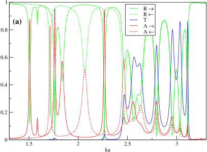
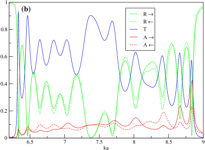
Figure 1: (Color online) Scattering process for disordered arrays of $15$ deltas with complex couplings. The sequences of the real parts of the characteristic parameters are: (a) $\textrm{Re}(a/a_{j})$: $3,1,2,0.5,3,2,1,3,0.5,4,5,1,2,2,3$ (b) $\textrm{Re}(a/a_{j})$:$-1,-4,-3,-1,-2,-3,-4,$ $-1,-2,-3,-1,-4,-4,-2,-3$ . The imaginary part of each coupling has been chosen as $\textrm{Im}(a/a_{j})=-0.01|\textrm{Re}(a/a_{j})|$. The arrows in the legends mark the direction of incidence.

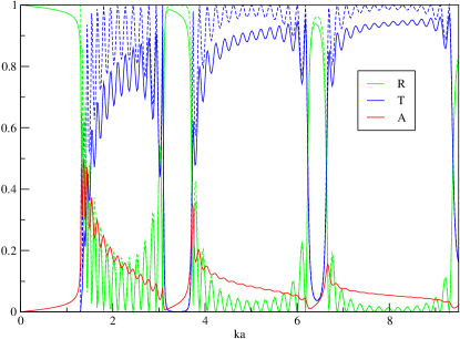
Figure 2: (Color online) Scattering and absorption probabilities for one-species delta chains with length $N=15$ and parameters $(a/a_{1})=1.0$ (dashed lines) and $(a/a_{1})=1.0-0.015i$ (solid lines).

Let us now incorporate the dissipative processes that are always present in real wires, causing energy losses. We have modelled that effect by including an imaginary part in the potential. In this case the natural complex extension of our system consists in promoting the delta couplings from real to complex, thus writing $(a/a_{j})=r_{j}-is_{j}$. We also take $s_{j}>0$ for all $j$ in order to avoid anomalous scattering. The effect of including complex couplings on the spectrum of an infinite periodic delta chain has recently been studied in detail ptcer . Let us see what happens in a chain with open boundaries. In Fig.2 the usual scattering diagram is shown for a short periodic chain with real potentials. Including a small imaginary part in the couplings we see how the transmission pattern is altered with a non-negligible absorption that peaks at the incoming band edges while the reflectivity is not noticeably changed. This tendency of the absorption term also appears when several species are included in the periodic array, and its pattern does not change much if only some of the couplings are complexified.

When the array presents no ordering at all, the graph is quite unpredictable and different configurations can be obtained. In Fig.1(a) a peaky spectrum with very sharp absorption resonances is shown. The scattering process in this case is strongly dependent on the direction incidence, as can be seen. On the other hand, smoother diagrams are also possible in which the effect of the complex potential manifests through an almost constant absorption background and a small change depending upon the colliding side, like the one in Fig.1(b).

This naive potential, apart from being exactly solvable, is powerful enough to account for very different physical schemes, which makes it a very useful bench-proof structure.

V Atomic quantum wells

Let us go one step further and consider a potential that resembles the profile of an atomic quantum well with analytical solutions, the well-known Pöschl-Teller potential hole. It reads,

$$V(x)=-\frac{\hbar^{2}}{2m}\alpha^{2}\frac{\lambda(\lambda-1)}{\cosh^{2}(\alpha x)}\quad\lambda>1,$$ (14)

and it is shown in Fig.3.

Figure 3: Pöschl-Teller potential (arbitrary units).

The probability of asymptotic transmission is well knownflugge ,

$$T_{PT}(k)=\frac{1}{1+p^{2}}\quad;\quad p=\frac{\sin(\pi\lambda)}{\sinh(k\pi/\alpha)}.$$ (15)

One characteristic feature of the Pöschl-Teller hole is that it behaves as an absolute transparent potential for integer values of $\lambda$, as can be seen from Eq.(15). From the wave functions one can also obtain the asymptotic transmission matrix,

$$\mathbf{M}_{PT}(k)=\begin{pmatrix}ie^{i\gamma}\sqrt{1+p^{2}}&-ip\\ ip&-ie^{-i\gamma}\sqrt{1+p^{2}}\end{pmatrix}$$ (16)

where $\gamma=2\arg\Gamma(ik/\alpha)-\arg\{\Gamma(\lambda+ik/\alpha)\Gamma(1-\lambda+ik/\alpha)\}$.

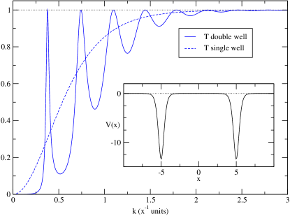
Figure 4: (Color online) Transmission through a double Pöschl-Teller hole with parameters $\alpha_{1}=\alpha_{2}=2$ ($x^{-1}$ units), $\lambda_{1}=\lambda_{2}=2.4$, $d_{1}=d_{2}=5$ ($x$ units). The dashed line corresponds to a single potential hole. The inset shows the composite potential profile (arbitrary units).

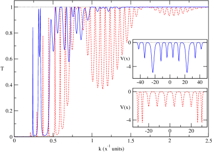
Figure 5: (Color online) Transmission patterns for two symmetric composite potentials of ten units each. Their profiles are shown in the insets (arbitrary units). Parameters for the first five potentials of the sequences: (solid line) $\alpha=1,1,0.5,1,1$($x^{-1}$ units), $\lambda=1.66,2.19,5.01,2.33,2.16$, $d=4,4,7,4,4$($x$ units) and (dashed line) $\alpha=2,2,1,1,1$($x^{-1}$ units), $\lambda=1.66,1.66,2.03,2.03,2.03$, $d=2,2,4,4,4$($x$ units).

Let us try to build a chain with these atomic units. In order to do so, one has to include a sensible cut-off in the potentials to ensure first that the wave function takes a proper form at the junction regions and second that the resulting potential hole can still be described by a handy transmission matrix, so that Eqs.(4) can be applied easily. The cut-off will be placed at a distance $d$ from the center of the potential (Fig.3). The wave function in the interval $[-d,d]$ is $\Psi_{2}(x)=A_{2}e(x)+B_{2}o(x)$ where $e(x),o(x)$ are the even and odd solutions respectively of the Schrödinger equation. Outside that interval the wave function is assumed to be a superposition of the free particle solutions, regions 1 and 3 in Fig.3. The connection equations at the cut-off points lead to a relationship between the amplitudes of the wave function in sectors 1 and 3 in terms of the values of $e(x),o(x)$ and their spatial derivatives at $\pm d$. Therefore, the distance $d$ must be such that the asymptotic form of the solutions of the Schrödinger equation can be used at that point in order to ensure a sensible transition to the free particle state and to obtain a transmission matrix as simple as possible. The solutions $e(x),o(x)$ as well as their asymptotic forms are found in Reference flugge, ; nevertheless they are also reproduced in Appendix A.

After some algebra one finds the transmission matrix for the cut-off version of the potential hole,

$$\mathbf{M}(k)=\begin{pmatrix}ie^{i(\gamma+2kd)}\sqrt{1+p^{2}}&-ip\\ ip&-ie^{-i(\gamma+2kd)}\sqrt{1+p^{2}}\end{pmatrix}.$$ (17)

The matrix is the same as for the asymptotic case in Eq.(16) plus an extra phase term in the diagonal elements that accounts for the distance $2d$ during which the particle feels the effect of the potential. These phases are the key quantities for the composition procedure since they will be responsible for the interference processes that produce the transmission patterns. Due to the rapid decay of the Pöschl-Teller potential, the distance $d$ admits very reasonable values. In fact, we have seen that for a sensibly wide range of the parameters $\alpha\in[0.1,3]$, $\lambda\in[1,5]$ one can take as a minimum value for the cut-off distance $d_{0}\simeq 2d_{1/2}=3.5/\alpha$, where $d_{1/2}$ is the half-width (Fig.3). Taking $d\geq d_{0}$ the connection procedure works really well, as we have checked in all cases by comparing the analytical composition technique versus a high precision numerical integration of the Schrödinger equation, obtaining an excellent degree of agreement.

Composing two potential holes and applying Eqs.(4) together with Eq.(17) one finds for the transmission probability, using the previously defined quantities $p$,$\gamma$

$$T_{2PT}(k)=\frac{1}{p_{1}^{2}p_{2}^{2}+(1+p_{1}^{2})(1+p_{2}^{2})-2p_{1}p_{2}\sqrt{1+p_{1}^{2}}\sqrt{1+p_{2}^{2}}\cos(\gamma_{1}+\gamma_{2}+2k(d_{1}+d_{2}))},$$ (18)

which is a handy expression that can hardly be obtained by trying to solve the Schrödinger equation for the double potential hole. To our knowledge this calculation has not been made before. Eq.(18) clearly shows the interference effect depending on the distance $d_{1}+d_{2}$ between the centers of the holes. An example of transmission is shown in Fig.4.

The composition procedure can be applied with a small number of atoms to study the transmitivity of different potential profiles resembling molecular structures such as those in Fig.5. The transmission matrix (17) can also be used to consider a continuous disordered model in the form of a large chain of these potential holes with random parameters. So far, in the literature only two kinds of potentials have been used to build continuous disordered models, namely the Dirac delta potential and the square well(barrier), due to their well known and easy to manipulate transmission matrices. We recall the fact that handy transmission matrices can be obtained for other potential profiles using reasonable approximations, such as the one described here.

The next step for our purpose is to consider dissipation in these one-dimensional composite potentials.

VI Dissipative atomic quantum wells/barriers

We shall consider the extension of the Pöschl-Teller potential given by the complexified Scarf potential,

$$V(x)=\frac{\hbar^{2}\alpha^{2}}{2m}\left(\frac{V_{1}}{\cosh^{2}(\alpha x)}+i\,V_{2}\frac{\sinh(\alpha x)}{\cosh^{2}(\alpha x)}\right)$$ (19)

with $V_{1},V_{2}\,\in\mathbb{R}$. It is a proper complex extension for two reasons: it admits analytical solutions avinash and its imaginary part is somehow proportional to the derivative of the real potential. This latter criterion has been considered in nuclear optical potentials to choose adequate complex extensions. It seems reasonable to measure the strength of the dissipation processes in terms of the “density” of the real interaction and therefore writing an imaginary potential that is proportional to the spatial derivative of the real one. The potential profile is shown in Fig.6.

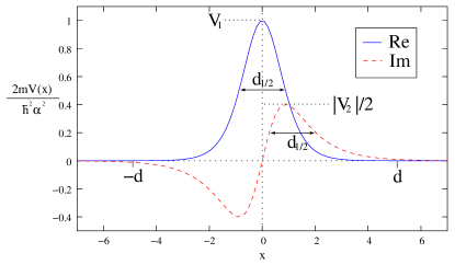
Figure 6: Real and imaginary parts of the complex Scarf potential (arbitrary units).

The Scarf potential has been extensively considered in the literature, mainly dealing with its discrete spectrum, either in its real and complex forms, from the point of view of SUSY Quantum Mechanics susy or focusing on its $\mathcal{PT}$-symmetric form ahmed .

First, a detailed mathematical analysis of the potential, regarding its scattering properties, must be made to discuss some new features and some assertions that have been made.

The left scattering amplitudes of the real Scarf potential have been obtained in terms of complex Gamma functions avinash . Recently, a considerable simplification has been pointed out by Ahmedahmed . In fact, the asymptotic transmitivity and reflectivity for the complex Scarf can be written as,

$$T(k) =\frac{\sinh^{2}(2\pi k/\alpha)}{\sinh^{2}(2\pi k/\alpha)+2\cosh(2\pi k/\alpha)\cosh(\pi g_{+})\cosh(\pi g_{-})+\cosh^{2}(\pi g_{+})+\cosh^{2}(\pi g_{-})}$$ (20)

$$R^{L}(k) =\frac{\cosh^{2}(\pi g_{+})e^{-2\pi k/\alpha}+\cosh^{2}(\pi g_{-})e^{2\pi k/\alpha}+2\cosh(\pi g_{+})\cosh(\pi g_{-})}{\sinh^{2}(2\pi k/\alpha)+2\cosh(2\pi k/\alpha)\cosh(\pi g_{+})\cosh(\pi g_{-})+\cosh^{2}(\pi g_{+})+\cosh^{2}(\pi g_{-})}$$ (21)

where $g_{\pm}=\sqrt{V_{1}\pm V_{2}-1/4}$ and $R^{R}(k)$ is recovered from $R^{L}(k)$ by interchanging $g_{+}$ and $g_{-}$ (which is equivalent to substituting $V_{2}\rightarrow-V_{2}$ and therefore changing the direction of incidence). These expressions derive from the asymptotic transmission matrix, which is obtained here using the asymptotic form of the Schrödinger equation solutions (Appendix B),

$$M_{Scarf}(k)=\begin{pmatrix}ie^{i\varphi}\sqrt{1+s\overline{s}}&-is\\ i\,\overline{s}&-ie^{-i\varphi}\sqrt{1+s\overline{s}}\end{pmatrix}$$ (22)

where

$$s =\frac{\cosh(\pi g_{+})e^{\pi k/\alpha}+\cosh(\pi g_{-})e^{-\pi k/\alpha}}{\sinh(2\pi k/\alpha)}$$ (23)

$$\overline{s} =s(g_{+}\rightleftarrows g_{-})$$ (24)

and $\varphi=2\arg\{\Gamma(ik/\alpha)\Gamma(1/2+ik/\alpha)\}-\arg\{\Gamma(c+ik/\alpha)\Gamma(b+ik/\alpha)\Gamma(1-c+ik/\alpha)\Gamma(1-b+ik/\alpha)\}$ with the definitions

$$c=\frac{1}{2}-\frac{i}{2}(g_{+}-g_{-})\quad;\quad b=\frac{1}{2}-\frac{i}{2}(g_{+}+g_{-}).$$ (25)

It immediately follows from the transmission matrix that the absorption probabilities read,

$$A^{L}(k)=\frac{s\overline{s}-\overline{s}^{2}}{1+s\overline{s}}\quad;\quad A^{R}(k)=\frac{s\overline{s}-s^{2}}{1+s\overline{s}}.$$ (26)

Unlike the complex delta potentials example this potential has some drawbacks that must be carefully solved. Its imaginary part is non-negative defined in its domain, which might cause anomalous scattering. Only some values of $V_{2}$ will be physically acceptable. To ensure that $T(k)\leq 1\quad\forall\,k$, it is clear from Eq.(20) that the necessary and sufficient condition is $\cosh(\pi g_{+})\cosh(\pi g_{-})\geq 0$. The functions $g_{+}$, $g_{-}$ can be real or pure imaginary depending on the values of $V_{1}$ and $V_{2}$. A detailed analysis of the conditions for physical transmission is presented in Appendix B. As a summary, let us say that for $V_{1}>0$ (barriers) , the evaluation of the condition translates into,

$$\begin{split}|V_{2}|\in&[0,V_{1}]\cup\\ &[2n(2n-1)+V_{1},2n(2n+1)+V_{1}]\quad n\in\mathbb{Z}^{+}.\end{split}$$ (27)

For $V_{1}<0$ (wells) the situation becomes more complicated and the result can only be expressed through several inequalities, each one adding a certain allowed range for $V_{2}$ (see Appendix B). As an example, in Table 1 we show the compatible ranges of $V_{2}$ for a few negative values of $V_{1}$. One can trivially check the compatibility of the intervals presented for $V_{2}$ with the condition $T(k)\leq 1\quad\forall\,k$ by plotting Eq.(20). In a two dimensional plot of $|V_{2}|$ vs. $V_{1}$, the physical ranges for the transmission distribute as alternating fringes and a funny chessboard like pattern (Fig.9).

$V_{1}$	$|V_{2}|$	$|V_{2}|$ emissive
$-0.5$	$[0,0.5]\cup[1.5,5.5]\cup[11.5,19.5]\ldots$	$[0,0.5]$
$-1$	$[0,5]\cup[11,19]\cup[29,41]\ldots$	$\emptyset$
$-2.4$	$[0,0.4]\cup[2.4,3.6]\cup[9.6,17.6]\ldots$	$[0,0.4]\cup[2.4,2.569]$
$-3$	$[0,1]\cup\{3\}\cup[9,17]\ldots$	$[0,1]$
$-4$	$[0,4]\cup[8,16]\cup[26,38]\ldots$	$[3.606,4]$
$-5$	$[0,1]\cup[3,5]\cup[7,15]\ldots$	$[3,4.123]\cup[4.472,5]$

Table 1: Ranges of $V_{2}$ compatible with the condition $T(k)\leq 1\quad\forall\,k$ for the complex Scarf potential for certain negative values of $V_{1}$. The last column includes the intervals providing physical scattering from the emissive side of the potential.

One feature to emphasize according to the conditions given for acceptable transmission is the fact that the number of permitted intervals for $V_{2}$ is infinite for any $V_{1}$, either positive(barrier) or negative(well), and therefore there is no mathematical upper bound on $|V_{2}|$($|V_{2}^{critical}|$) above which the transmission probability always becomes unphysical, contrary to what has been reported recently ahmed . From a physical viewpoint of course, a sensible limitation must also be imposed on $V_{2}$, usually $|V_{2}|\ll|V_{1}|$.

Let us see now what happens with the reflectivity. We assert that for the values of $V_{1}$ and $V_{2}$ preserving a physical transmission, one of the reflectivities of the system remains physical (i.e. $R(k)\leq 1-T(k)\quad\forall\,k$), left or right, depending on the particular values of $V_{1},V_{2}$ (or equivalently, one of the absorptions takes positive values for all $k$). The statement is easy to prove from Eqs.(26) and more specifically reads: when $T(k)\leq 1\quad\forall\,k$ (i.e. $\cosh(\pi g_{+})\cosh(\pi g_{-})\geq 0$), then

$$\begin{split}|\cosh(\pi g_{-})|<|\cosh(\pi g_{+})|&\Rightarrow A^{L}(k)\geq 0\quad\forall\,k\\ |\cosh(\pi g_{-})|>|\cosh(\pi g_{+})|&\Rightarrow A^{R}(k)\geq 0\quad\forall\,k.\end{split}$$ (28)

Considering $V_{1}>0$ and $V_{2}>0$ it is not hard to see that the first of the above inequalities always holds. Therefore, in the case of a potential barrier the scattering is always physical from the absorptive side (trough of the imaginary part), as has already been stressed ahmed . More interesting is the fact that this conclusion cannot be extended to the case $V_{1}<0$ (well). In this case the physical scattering sometimes occurs from the emissive side (peak of the imaginary part), producing smaller absorption terms. In Table 1 a few examples of $V_{2}$ intervals providing physical scattering from the emissive side for some potential wells are shown.

Another interesting feature that must be observed is that there exists a set of correlated values of $V_{1},V_{2}$ for which the complex Scarf potential behaves as fully transparent. The condition for this to happen is from Eq.(20) $\cosh(\pi g_{+})=\cosh(\pi g_{-})=0$. Thus, the main requirement is that $g_{+},g_{-}$ must be pure imaginary, yielding in this case the transparency equations,

$$\cos\left(\pi\sqrt{\frac{1}{4}-V_{1}\pm V_{2}}\right)=0$$ (29)

whose solution is,

$$V_{1} =\frac{1}{4}-\frac{1}{8}\left[(2m+1)^{2}+(2n+1)^{2}\right]$$ (30a)

$$V_{2} =\frac{1}{8}\left[(2m+1)^{2}-(2n+1)^{2}\right]\quad m,n\in\mathbb{Z}.$$ (30b)

It is worth noting that the transparencies only appear for potential wells ($V_{1}<0$). Considering the particular case $n=m$ one recovers the Pöschl-Teller resonances ($\lambda\in\mathbb{Z}$). In Table 2 the first values of Eqs.(30) are listed explicitly.

		$(-V_{1}$,$|V_{2}|)$
$(1,1)$	$(3,3)$	$(6,6)$	$(10,10)$	$(15,15)$
$[2,0]$	$(4,2)$	$(7,5)$	$(11,9)$	$(16,14)$
$[6,0]$	$(9,3)$	$(13,7)$	$(18,12)$	$(24,18)$
$[12,0]$	$(16,4)$	$(21,9)$	$(27,15)$	$(34,22)$

Table 2: Some correlated values of $V_{1},V_{2}$ producing the fully resonant behaviour of the complex Scarf potential. The particular Pöschl-Teller resonances are in square brackets.

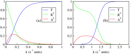
Figure 7: (Color online) Characteristic scattering patterns for (a) a complex Scarf well $\alpha=1$($x^{-1}$ units),$V_{1}=-0.5,V_{2}=-0.4$ and (b) a complex Scarf barrier $\alpha=1$($x^{-1}$ units),$V_{1}=2,V_{2}=0.1$.

The absorption obviously vanishes for all $k$ when considering these special resonant values of the potential amplitudes. Surprisingly, there also exists another set of non-trivial correlated values of $V_{1},V_{2}$ for which the potential is non-dissipative ($A(k)=0\quad\forall\,k$) without being fully transparent. This set of values satisfies $\cosh(\pi g_{+})=\cosh(\pi g_{-})\neq 0$, as can be seen from Eqs.(26). Non-trivial solutions exist when $g_{+},g_{-}\in\mathbb{C}$, yielding,

$$|V_{2}|=n\sqrt{1-4V_{1}-4n^{2}}\quad n\in\mathbb{Z}^{+}.$$ (31)

Let us also notice from Eqs.(28) that these solutions are also the borders where the physical scattering changes from the absorptive side to the emissive side or vice versa. We shall refer to these borders as inversion points (IP). Therefore, whenever we encounter an IP we can say $A(k)=0\quad\forall\,k$ without a fully transparent behaviour, and hence a non-dissipative scattering process for all energies with a non-vanishing imaginary part of the potential. Let us note that from Eq.(31) the IP only appears in the case of Scarf potential wells and only for $|V_{2}|\leq 1/4-V_{1}$. In Fig.7 the characteristic scattering probabilities are shown for a Scarf barrier and a Scarf well, and in Fig.8 the maximum value of the physical absorption is plotted versus $|V_{2}|$ for different values of $V_{1}$. When $V_{1}$ is positive the absorption grows with the amplitude of the imaginary part of the potential. On the other hand, for negative $V_{1}$ a strikingly different pattern arises, with transparencies (T) and inversion points (IP) and the absorption does not increase monotonically with $|V_{2}|$.

Figure 8: Maximum value of the absorption probability $A_{max}$ vs. $|V_{2}|$ for different values of $V_{1}$. For each graph the upper(lower) curve corresponds to a barrier(well). A dotted line is used in the forbidden values of $|V_{2}|$, nevertheless the whole curve is shown for continuity. The allowed ranges of $|V_{2}|$ and the position of the IP can be compared with the values in Table 1.

The whole behaviour of the scattering can be clearly understood by building a two dimensional diagram $|V_{2}|$ vs. $V_{1}$ (Fig.9), including physically permitted ranges, inversion lines and the points of transmission resonance. The complex Scarf potential shows two opposite faces to scattering, namely barrier and well, and a much richer structure in the latter case.

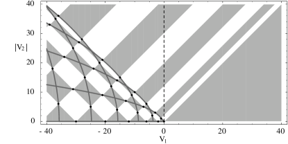
Figure 9: Scattering diagram for the complex Scarf potential in terms of the potential amplitudes. The physically acceptable ranges for $V_{1},V_{2}$ correspond to the shaded zones. The curves are the inversion lines given by Eq.(31). The black points mark the correlated values of the amplitudes (Eqs.(30)) generating a fully transparent behaviour.

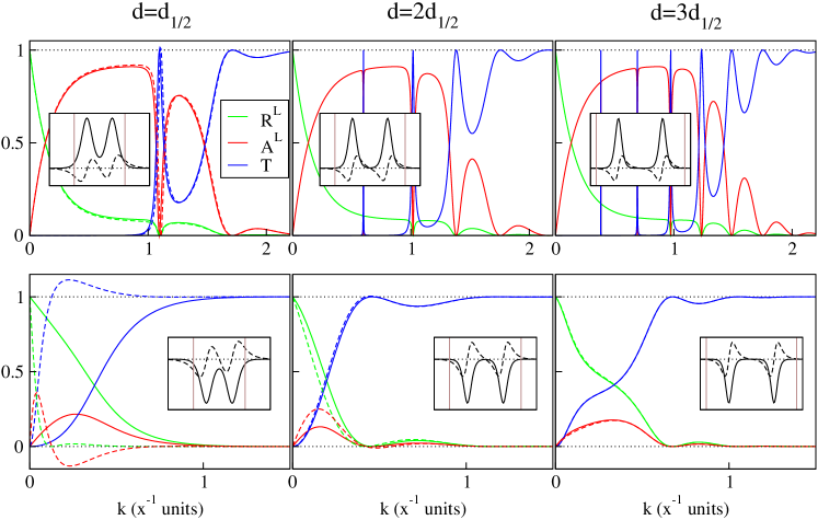
Figure 10: (Color online) Scattering probabilities for double Scarf potentials with parameters $\alpha=1$($x^{-1}$ units),$V_{1}=2,V_{2}=1$ for barriers and $\alpha=1$($x^{-1}$ units),$V_{1}=-4,V_{2}=3.1$ for wells. The solid lines were obtained from the analytical composition technique and the dashed lines correspond to the exact numerical integration of the Schrödinger equation. The insets show the potential profile (in arbitrary units) for each case: solid line for the real part and dashed for the imaginary part. The vertical lines limit the portion of the potential that the composition technique takes into account. For numerical integration the whole potential profile was considered. Notice that for low $d$ the exact integration may lead to unphysical scattering because the conditions obtained for physical scattering are not valid for such $d$ values. As $d$ is increased an acceptable scattering is recovered and both methods start converging. Convergence is reached faster in the case of potential barriers where the analytical composition technique works impressively well even for very low values of $d$.

After this detailed analysis of the peculiarities of the complex Scarf, that to our knowledge have not been reported before, let us continue with our work on connecting several potentials to model dissipative atomic chains. The procedure is the same as the one described for the Pöschl-Teller potential hole in Section V. Only the portion of the potential included in the interval $[-d,d]$ is taken (Fig.6). Making use of the asymptotic forms of the wave functions, and after some algebra, one finds the transmission matrix for the complex Scarf potential with a symmetrical cut-off,

$$M(k)=\begin{pmatrix}ie^{i(\varphi+2kd)}\sqrt{1+s\overline{s}}&-is\\ i\,\overline{s}&-ie^{-i(\varphi+2kd)}\sqrt{1+s\overline{s}}\end{pmatrix}.$$ (32)

The matrix proves to be the same as for the asymptotic case (Eq.(22)), but with the extra phase $2kd$ in the diagonal terms. It can be checked that the half-widths $d_{1/2}$ of both the real and imaginary parts coincide and that the decay of the imaginary part of the potential is always slower than that of the real part (Fig.6). This causes an increase in the minimum value of the cut-off distance $d_{0}$ with regard to the Pöschl-Teller case. For sensible values of the potential amplitudes we have found that considering $d_{0}\simeq 3d_{1/2}=5.3/\alpha$ is enough in most cases. In fact, this minimum value can be relaxed in the case of potential barriers ($V_{1}>0$), whereas for potential wells taking $d$ below this value to apply the connection equations may sometimes distort the results. The correct behaviour of the connection procedure for $d\geq d_{0}$ can be observed in Fig.10 where the scattering probabilities obtained upon integrating the Schrödinger equation numerically are compared with those given by the analytical composition technique, for two potential barriers and two potential wells with different choices of the cut-off distance and with high values for $|V_{2}|$. Notice how in the barrier example convergence between the methods is completely reached for $d\simeq 2d_{1/2}$ whereas for potential wells a further step is needed because the convergence is much slower.

Once the connection of potentials has been successfully made, one should ask which are the ranges of the potential amplitudes that provide an acceptable physical scattering in this new framework. Analysis of this issue is very non-trivial and quite complex analytically, but also very important because it determines whether this model remains useful when considering atomic chains. First, in the case of two potentials we have observed that choosing each individual pair of amplitudes $(V_{1},V_{2})$ belonging to a physical range, and selecting the signs of the imaginary parts so that the physical faces of both potentials point in the same direction, then an acceptable scattering for the composite potential can always be recovered at least from one of the two possible orientations (both physical faces to the right or to the left). In other words, considering that the incident particle always collides with the left side (it comes from $-\infty$) and therefore orientating the individual physical faces to the left, then at least one of the sequences $V_{I}(x)-V_{II}(x)$ or $V_{II}(x)-V_{I}(x)$ gives an acceptable scattering for all energies. We have checked this assertion for a broad variety of Scarf couples. For a higher number of potentials the situation becomes more complex but a few pseudo-rules to obtain physical scattering can be deduced. For an arbitrary chain we have found that in many cases the left scattering remains physical as long as: the left scattering of each individual potential is physical and the left scattering of each couple of contiguous potentials is physical. This recipe seems completely true when composing potential barriers only, whereas when wells are included it fails in some situations, especially when several contiguous wells are surrounded by barriers. Although at the beginning it may appear almost random to recover a physical scattering from a large composition of Scarfs, following the given advices it turns out to be more systematic.

Let us remember that the composition procedure, apart from being a powerful tool for numerical calculations also provides analytical expressions for the scattering probabilities, which of course adopt cumbersome forms for a large number of potentials but are useful for obtaining simple expansions for certain energetic regimes. Just as an example, the transmitivity and left reflectivity for the double Scarf read,

$$T_{2Scarf}(k) =\frac{1}{s_{1}^{2}\overline{s}_{2}^{2}+(1+s_{1}\overline{s}_{1})(1+s_{2}\overline{s}_{2})-2s_{1}\overline{s}_{2}\sqrt{1+s_{1}\overline{s}_{1}}\sqrt{1+s_{2}\overline{s}_{2}}\cos(\varphi_{1}+\varphi_{2}+2k(d_{1}+d_{2}))}$$ (33)

$$R^{L}_{2Scarf}(k) =\frac{\overline{s}_{1}^{2}(1+s_{2}\overline{s}_{2})+\overline{s}_{2}^{2}(1+s_{1}\overline{s}_{1})-2\overline{s}_{1}\overline{s}_{2}\sqrt{1+s_{1}\overline{s}_{1}}\sqrt{1+s_{2}\overline{s}_{2}}\cos(\varphi_{1}+\varphi_{2}+2k(d_{1}+d_{2}))}{s_{1}^{2}\overline{s}_{2}^{2}+(1+s_{1}\overline{s}_{1})(1+s_{2}\overline{s}_{2})-2s_{1}\overline{s}_{2}\sqrt{1+s_{1}\overline{s}_{1}}\sqrt{1+s_{2}\overline{s}_{2}}\cos(\varphi_{1}+\varphi_{2}+2k(d_{1}+d_{2}))}$$ (34)

making use of the previously defined terms $s,\overline{s}$ and $\varphi$. One important feature of the formulae for the composite scattering probabilities is the fact that they analytically account for the fully transparent behaviour of the whole structure as long as there is resonant forward scattering of the individual potential units, as can be seen from the latter equations and also from Eq.(18) for the double Pöschl-Teller. Another curious feature arises when composing different potentials whose amplitudes describe an IP. In this case the whole structure remains non-dissipative (Fig.11). Moreover, the complex Scarfs at these points behave completely as real potentials, providing an acceptable scattering for the composition that is independent of the incidence direction for any sequence of the individual Scarfs.

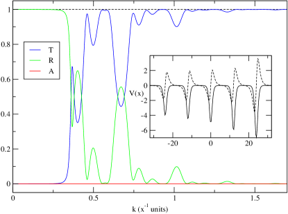
Figure 11: (Color online) Composition of Scarfs with different pair amplitudes describing IPs. Sequence with $\alpha=1$($x^{-1}$ units) and $(V_{1},V_{2})$: $(-4,\sqrt{13})$, $(-4.5,\sqrt{15})$, $(-5,\sqrt{17})$, $(-6,\sqrt{21})$, $(-7,2\sqrt{13})$. All the cut-off distances have been taken equal to $d=6$($x$ units). The inset shows the potential profile with solid(dashed) line for the real(imaginary) part in arbitrary units. Notice that the composition remains non-dissipative.

Considering larger Scarf chains with small imaginary parts of the potentials, in the case of a periodic array we observe that the absorption term remains flat over a wide range of forbidden bands and oscillates inside the permitted ones. The variations in the absorption are entirely balanced by the reflectivity while the transmitivity is surprisingly not affected by the presence of a small complex potential (Fig.12). This behaviour contrasts strongly with the complex delta potentials periodic chain where the absorption was completely different and it was the reflectivity that was little affected by the dissipation.

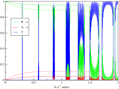
Figure 12: (Color online) Periodic chain of $20$ complex Scarfs with amplitudes $\alpha=1$($x^{-1}$ units), $V_{1}=2$, $V_{2}=0.02$ (solid lines) and $V_{2}=0.05$ (dashed lines) and cut-off distance $d=6$($x$ units). The transmitivity is not changed much by the small imaginary part of the potentials.

For an aperiodic sequence the situation is quite different, as expected. In Fig.13 a type of molecular aggregate is modelled with complex Scarfs. It exhibits a peaky absorption spectrum and a strongly oscillating transmitivity with sharp resonances. In Fig.14 a symmetric atomic cluster has been considered in which the dissipation only occurs at both ends. Different transmission and absorption configurations can be obtained by building different structures. This shows the usefulness and versatility of this model for being able to account for a variety of possible experimental observations.

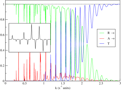
Figure 13: (Color online) Scattering probabilities for a $10$-Scarf structure with parameters $\alpha=1$($x^{-1}$ units) and $(V_{1},V_{2})$: $(1,0)$, $(-0.5,-0.005)$, $(-1.3,0.013)$, $(1.8,0.01)$, $(-1.3,0.013)$, $(4,0.04)$, $(-2.4,-0.024)$, $(3.5,0.04)$, $(-3.1,0.031)$, $(-1.5,0.04)$. The cut-off distance is $d=6$($x$ units) equal for all of them. The inset shows the real part of the potential profile (arbitrary units).

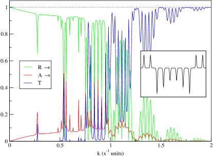
Figure 14: (Color online) Scattering probabilities for a $10$-Scarf structure with parameters $\alpha=1$($x^{-1}$ units) and $(V_{1},V_{2})$: $(1,0.04)$, $(1,0.05)$, $(-2,0)$, $(-1.5,0)$, $(-1,0)$, $(-1,0)$, $(-1.5,0)$, $(-2,0)$, $(1,0.1)$, $(1,0.1)$. The cut-off distance is $d=6$($x$ units) equal for all of them. The inset shows the real part of the potential profile (arbitrary units).

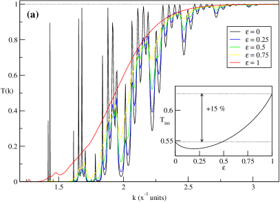
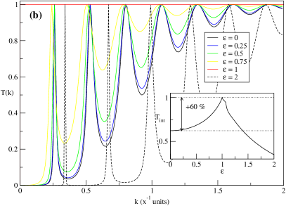
Figure 15: (Color online) Transmitivity for different strengths of the imaginary part of the potentials in (a) a chain of 6-Scarf barriers $V_{1}=4,2,2.5,3,3.5,4$ and $\alpha=1$($x^{-1}$ units), (b) a double Scarf well with $V_{1}=-1,-1$ and $\alpha=2$($x^{-1}$ units). The cut-off distances in all cases are equal to $d=6$($x$ units). Each imaginary amplitude reads $V_{2}=\varepsilon|V_{1}|$, except the first barrier in example (a) which is maintained real. The insets show the evolution of $T_{int}$ vs the strength of the imaginary amplitudes.

As a final exercise, two examples are included in Fig.15 showing the evolution of the transmitivity of two different Scarf compositions as a function of the imaginary part of the potential. The transmission patterns are plotted for different values of the parameter $\varepsilon=|V_{2}|/|V_{1}|$, which measures the strength of the imaginary part. The transmission efficiency is evaluated using an averaged transmitivity $T_{int}=\int_{k_{1}}^{k_{2}}T(k)\,dk/(k_{2}-k_{1})$ corresponding to the area enclosed by $T(k)$ per energy unit in a characteristic energy range, namely the zone where $T$ evolves until it becomes saturated. The imaginary potential tends to smooth the transmission pattern in the first example (corresponding to a sequence of barriers), causing a slight decrease in the averaged transmitivity for low $\varepsilon$, although it is finally improved. For a double well a different effect occurs. $T_{int}$ is always enhanced with increasing $\varepsilon$ until it reaches a maximum, after which the transmitivity falls with the imaginary potential. With these results in mind one could speculate that these models might also be useful to describe the phase-breaking inelastic scattering processes in atomic chains. Especially when one treats disordered arrays where the break of the localization regime could arise as a result of the loss of coherence due to inelastic collisions.

VII Concluding remarks

In this work we have used the transfer matrix formalism in the form of the multiple collision technique to model dissipative scattering processes by using complex potentials in various models of atomic chains. The absorption probability has been rigorously included to recover unitarity for the non-hermitian hamiltonians.

New exact analytical expressions are given for the scattering amplitudes of an arbitrary chain of delta potentials. The absorption effects arising by promoting the delta couplings to the complex domain have been shown, revealing the flexibility of this simple model to account for very different physical schemes.

Handy expressions for the transmission matrices of the Pöschl-Teller and the complex Scarf potential have been constructed in their asymptotic as well as their cut-off versions for the first time. These latter matrices have made feasible, via the composition technique, the assembly of an arbitrary number of potentials to build atomic one-dimensional wires that can incorporate absorptive processes. Different absorption configurations are presented in several examples that show the versatility of the model to account for a variety of possible experimental observations. The procedure developed is not only useful for numerical calculations but also provides analytical formulae for the composite scattering probabilities, which have not been obtained by other methods, and whose significance has been checked by numerical integrations of the Schrödinger equation.

From a more mathematical view, a complete and rigorous analysis of the scattering properties of the complex Scarf potential has been carried out. The ranges of physical transmission have been obtained and a group of novel features have arisen such as the presence of perfect transparencies and inversion points.

Apart from being able to include dissipation in the systems in a tractable way, the tools and methods provided may have direct applicability for considering molecular aggregates molecule and other structures with explicit potential profiles and also to build a new kind of continuous disordered models.

Future work seems promising since we are already in progress on the assembly of the one-dimensional structures to quantum dots in order to analyze the effect of dissipation on the conductance. Our aim is also to treat long disordered wires within this framework, and in particular to study the applicability of these potentials to account for the loss of coherence due to inelastic scattering process in the electronic localization regime.

Appendix A Solutions of the Pöschl-Teller potential

The elementary positive energy solutions of the Schrödinger equation with potential (14) read,

$$e(x)= \cosh^{\lambda}(\alpha x)F\left(a,b,\frac{1}{2};-\sinh^{2}(\alpha x)\right)$$ (35a)

$$o(x)= \sinh(\alpha x)\cosh^{\lambda}(\alpha x)\times$$

$$F\left(a+\frac{1}{2},b+\frac{1}{2},\frac{3}{2};-\sinh^{2}(\alpha x)\right)$$ (35b)

where $a=\frac{\lambda}{2}+i\frac{k}{2\alpha}$, $b=\frac{\lambda}{2}-i\frac{k}{2\alpha}$ and $F(a,b,c;z)$ is the Hypergeometric function. And their asymptotic forms can be written as,

$$e(x)\rightarrow \,me^{-i\varphi}e^{-ik|x|}+me^{i\varphi}e^{ik|x|}$$ (36a)

$$o(x)\rightarrow \,\textrm{sign}(x)\left(ne^{-i\theta}e^{-ik|x|}+ne^{i\theta}e^{ik|x|}\right)$$ (36b)

where

$$me^{i\varphi}= \frac{\sqrt{\pi}\,\Gamma\left(i\frac{k}{\alpha}\right)2^{-i\frac{k}{\alpha}}}{\Gamma\left(\frac{\lambda}{2}+i\frac{k}{2\alpha}\right)\Gamma\left(\frac{1-\lambda}{2}+i\frac{k}{2\alpha}\right)}$$ (37a)

$$ne^{i\theta}= \frac{\sqrt{\pi}\,\Gamma\left(i\frac{k}{\alpha}\right)2^{-i\frac{k}{\alpha}}}{2\,\Gamma\left(\frac{\lambda+1}{2}+i\frac{k}{2\alpha}\right)\Gamma\left(1-\frac{\lambda}{2}+i\frac{k}{2\alpha}\right)}.$$ (37b)

Appendix B Complex Scarf potential

B.1 Scattering states

The elementary positive energy solutions of the Schrödinger equation with the complex Scarf potential (19) are,

$$u_{1}(x)= e^{-i\left(b-\frac{1}{2}\right)\arctan(\sinh(\alpha x))}\cosh^{c}(\alpha x)\times$$

$$F\left(c+i\frac{k}{\alpha},c-i\frac{k}{\alpha},1-b+c;\frac{1}{2}+\frac{i}{2}\sinh(\alpha x)\right)$$ (38a)

$$u_{2}(x)= e^{-i\left(b-\frac{1}{2}\right)\arctan(\sinh(\alpha x))}\cosh^{c}(\alpha x)\times$$

$$\left(\frac{1}{2}+\frac{i}{2}\sinh(\alpha x)\right)^{b-c}\times$$

$$F\left(b+i\frac{k}{\alpha},b-i\frac{k}{\alpha},1+b-c;\frac{1}{2}+\frac{i}{2}\sinh(\alpha x)\right)$$ (38b)

$F(a,b,c;z)$ being the hypergeometric function and using the $b,c$ definitions in (25). The asymptotic limit $x\rightarrow\pm\infty$ yields,

$$u_{1}(x) \rightarrow 2^{c}\left[\textrm{sign}(x)\cdot i\right]^{\frac{1}{2}-b+c}\left(w_{1}e^{-ik|x|}+w_{2}e^{ik|x|}\right)$$ (39a)

$$u_{2}(x) \rightarrow-\,2^{c}\left[-\textrm{sign}(x)\cdot i\right]^{\frac{3}{2}-b+c}\left(q_{1}e^{-ik|x|}+q_{2}e^{ik|x|}\right)$$ (39b)

where

$$w_{1} =\frac{2^{2i\frac{k}{\alpha}}\Gamma\left(1-b+c\right)\Gamma\left(-2i\frac{k}{\alpha}\right)e^{-\textrm{sign}(x)\frac{\pi}{2}\frac{k}{\alpha}}}{\Gamma\left(c-i\frac{k}{\alpha}\right)\Gamma\left(1-b-i\frac{k}{\alpha}\right)}$$ (40a)

$$w_{2} =\frac{2^{-2i\frac{k}{\alpha}}\Gamma\left(1-b+c\right)\Gamma\left(2i\frac{k}{\alpha}\right)e^{\textrm{sign}(x)\frac{\pi}{2}\frac{k}{\alpha}}}{\Gamma\left(c+i\frac{k}{\alpha}\right)\Gamma\left(1-b+i\frac{k}{\alpha}\right)}$$ (40b)

$$q_{1} =w_{1}\left(b\rightleftarrows c\right)$$ (40c)

$$q_{2} =w_{2}\left(b\rightleftarrows c\right).$$ (40d)

B.2 Physical transmission

The condition for physical transmission is $\cosh(\pi g_{+})\cosh(\pi g_{-})\geq 0$. $V_{2}$ can be considered positive with no loss of generality since its change in sign (which is equivalent to changing the side of incidence) does not affect the transmission. With the definitions $X=|V_{1}|-V_{2}$ and $Y=|V_{1}|+V_{2}$, the study can be easily carried out. Considering $V_{1}>0$ the inequality translates into the permitted regions

$$\forall\quad Y\begin{cases}X>0\\ -2n(2n+1)\leq X\leq-2n(2n-1)\quad n\in\mathbb{Z}^{+}\end{cases}$$ (41)

which is clearly a sequence of allowed vertical fringes in the negative $X$ quadrant and the whole positive $X$ quadrant. This pattern will be same but rotated $\pi/4$ clockwise when the change of variables is undone. More specifically, in terms of the potential amplitudes the allowed intervals can be written as

$$\begin{split}|V_{2}|\in&[0,V_{1}]\cup\\ &[2n(2n-1)+V_{1},2n(2n+1)+V_{1}]\quad n\in\mathbb{Z}^{+}.\end{split}$$ (42)

In the case of $V_{1}<0$ a careful analysis leads to the following cumbersome allowed sets

$$X<0 \Rightarrow 2n(2n-1)\leq Y\leq 2n(2n+1)\quad n=1,2,3,\ldots$$ (43)

$$X>0 \Rightarrow\begin{cases}\big{\{}2n(2n-1)\leq X\leq 2n(2n+1)\big{\}}\bigcap\big{\{}2m(2m-1)\leq Y\leq 2m(2m+1)\big{\}}\quad n,m=1,2,\ldots\\ \big{\{}2j(2j+1)\leq X\leq 2j(2j+3)+2\big{\}}\bigcap\big{\{}2k(2k+1)\leq Y\leq 2k(2k+3)+2\big{\}}\quad k,j=0,1,2,\ldots\end{cases}$$ (44)

which are a set of allowed horizontal fringes in the negative $X$ quadrant and a chessboard like structure for positive $X$. Undoing the change of variables will mean a $\pi/4$ clockwise rotation followed by a reflection around the vertical axis of this pattern to recover the negative axis of $V_{1}$. Solving these inequalities in terms of the potential amplitudes gives rise to the following set of inequalities, each one assigning a certain allowed interval for $|V_{2}|$ when fulfilled, for $n\in\mathbb{Z}^{+}$,

$$\begin{split}|V_{1}|\leq n(2n-1)&\Rightarrow\big{[}2n(2n-1)-|V_{1}|,2n(2n+1)-|V_{1}|\big{]}\\ n(2n-1)\leq|V_{1}|\leq n(2n+1)&\Rightarrow\big{[}|V_{1}|,2n(2n+1)-|V_{1}|\big{]}\end{split}$$ (45)

for $m,n\in\mathbb{Z}^{+}\quad m\geq n$,

$$\begin{split}m(2m-1)+n(2n-1)\leq|V_{1}|\leq m(2m-1)+n(2n+1)&\Rightarrow\big{[}2m(2m-1)-|V_{1}|,-2n(2n-1)+|V_{1}|\big{]}\\ m(2m-1)+n(2n+1)\leq|V_{1}|\leq m(2m+1)+n(2n-1)&\Rightarrow\big{[}-2n(2n+1)+|V_{1}|,-2n(2n-1)+|V_{1}|\big{]}\\ m(2m+1)+n(2n-1)\leq|V_{1}|\leq m(2m+1)+n(2n+1)&\Rightarrow\big{[}-2n(2n+1)+|V_{1}|,2m(2m+1)-|V_{1}|\big{]}\end{split}$$ (46)

and for $j,k=0,1,2,\ldots\quad k\geq j$,

$$\begin{split}k(2k+1)+j(2j+1)\leq|V_{1}|\leq k(2k+1)+j(2j+3)+1&\Rightarrow\big{[}2k(2k+1)-|V_{1}|,-2j(2j+1)+|V_{1}|\big{]}\\ k(2k+1)+j(2j+3)+1\leq|V_{1}|\leq k(2k+3)+1+j(2j+1)&\Rightarrow\big{[}-2-2j(2j+3)+|V_{1}|,-2j(2j+1)+|V_{1}|\big{]}\\ k(2k+3)+1+j(2j+1)\leq|V_{1}|\leq k(2k+3)+j(2j+3)+2&\Rightarrow\big{[}-2-2j(2j+3)+|V_{1}|,2+2k(2k+3)-|V_{1}|\big{]}.\end{split}$$ (47)

In the particular cases $m=n$ for Eqs.(46) and $k=j$ for Eqs.(47) only the positive part of the allowed intervals must be considered. The total physical range for $|V_{2}|$ comes from the union of the different permitted intervals.

References

- (1) N. Agraït, C. Untiedt, G. Rubio-Bollinger and S. Vieira, Phys. Rev. Lett. 88, 216803 (2002)
- (2) M. Büttiker, Phys. Rev. B 32, 1846 (1985); M. Büttiker, Phys. Rev. B 33, 3020 (1986)
- (3) K. Maschke and M. Schreiber, Phys. Rev. B 44, 3835 (1991); Phys. Rev. B 49, 2295 (1994); R. Hey, K. Maschke and M. Schreiber, Phys. Rev. B 52, 8184 (1995)
- (4) J. M. Cerveró and A. Rodríguez, Eur. Phys. J. B 30, 239 (2002); Eur. Phys. J. B 32, 537 (2003)
- (5) J. L. D’Amato and H. M. Pastawski, Phys. Rev. B 41, 7411 (1990);
- (6) G. Czycholl and B. Kramer, Solid State Commun. 32, 945 (1979); D. J. Thouless and S. Kirkpatrick, J. Phys. C 14, 235 (1981)
- (7) V. Freilikher et al, Phys. Rev. Lett. 73, 810 (1994); F. Delgado, J. G. Muga and A. Ruschhaupt, Phys. Rev. A 69, 022106 (2004)
- (8) L. I. Deych et al, Phys. Rev. B 64, 024201 (2001)
- (9) C. Dembowski et al, Phys. Rev. Lett. 86, 787 (2001); W. D. Heiss, Phys. Rev. E 61, 929 (2000)
- (10) W. D. Heiss, J. Phys. A 37, 2455 (2004); Eur. Phys. J. D 7, 1 (1999); W. D. Heiss and H. L. Harney, Eur. Phys. J. D 17, 149 (2001); Eur. Phys. J. D 29, 429 (2004)
- (11) N. Hatano and D. R. Nelson, Phys. Rev. Lett. 77, 570 (1996); Phys. Rev. B 56, 8651 (1997)
- (12) C. M. Bender and S. Boettcher, Phys. Rev. Lett. 80, 5243 (1998) ; C. M. Bender et al, J. Phys. A 40, 2201 (1999);R. M. Deb et al, Phys. Lett. A 307, 215 (2003);
- (13) J. M. Cerveró, Phys. Lett. A 317, 26 (2003); J. M. Cerveró and A. Rodríguez, J. Phys. A. In Press quant-ph/0312163 ; Z. Ahmed, Phys. Lett. A 286, 231 (2001)
- (14) C. Bender, G. V. Dunne and P. N. Meisinger, Phys. Lett. A 252, 272 (1999); A. Khare and U. P. Sukhatme, Phys. Lett. A 324, 406 (2004)
- (15) T. Khalil and J. Richert, J. Phys. A 37, 4851 (2004)
- (16) J. G. Muga, J. P. Palao, B. Navarro and I. L. Egusquiza, Phys. Rep. 395, 357 (2004)
- (17) P. Harrison, Quantum wells, wires and dots John Wiley and Sons Ltd, (2000)
- (18) Z. Ahmed, Phys. Rev. A 64, 042716 (2001)
- (19) J. E. Beam, Am. J. Phys. 38, 1395 (1970)
- (20) J. P. Palao, J. G. Muga and R. Sala, Phys. Rev. Lett. 80 5469 (1998)
- (21) A. Sánchez, E. Maciá and F. Dominguez-Adame, Phys. Rev. B 49, 147 (1994)
- (22) S. Flügge, Practical quantum mechanics, Springer-Verlag, Berlin (1970)
- (23) A. Khare and U. P. Sukhatme, J. Phys. A 21, L501 (1988); J. W. Dabrowska, A. Khare and U. P. Sukhatme, J. Phys. A 21, L195 (1988)
- (24) J. M. Cerveró, Phys. Lett. A 153, 1 (1991); G. Lévai and M. Znojil, J. Phys. A 35, 8793 (2002)
- (25) Z. Ahmed, Phys. Lett. A 324, 152 (2004)
- (26) R. Hey, F. Gagel, M. Schreiber and K. Maschke, Phys. Rev. B 55, 4231 (1997)