Quantum transport through a deformable molecular transistor

Abstract

The linear transport properties of a model molecular transistor with electron-electron and electron-phonon interactions were investigated analytically and numerically. The model takes into account phonon modulation of the electronic energy levels and of the tunnelling barrier between the molecule and the electrodes. When both effects are present they lead to asymmetries in the dependence of the conductance on gate voltage. The Kondo effect is observed in the presence of electron-phonon interactions. There are important qualitative differences between the cases of weak and strong coupling. In the first case the standard Kondo effect driven by spin fluctuations occurs. In the second case, it is driven by charge fluctuations. The Fermi-liquid relation between the spectral density of the molecule and its charge is altered by electron-phonon interactions. Remarkably, the relation between the zero-temperature conductance and the charge remains unchanged. Therefore, there is perfect transmission in all regimes whenever the average number of electrons in the molecule is an odd integer.

I Introduction

There has been in recent years a surge of interest in the study of transport phenomena in nanoscale systems motivated by their potential as electronic devices. These systems differ fundamentally from conventional conductors in that their electronic spectrum is discrete and their charging energies can not be ignored.

Charging effects on the transport properties have been intensively studied. Coulomb blockade has been observed in the conductance of quantum dots Klein et al. (1997) and in single-molecule devices weakly coupled to the electrodes. Park et al. (2002); Kubatkin et al. (2003) The enhancement of the low-temperature conductance in the valley between Coulomb blockade peaks due to the Kondo effect has also been observed both in quantum dots Goldhaber-Gordon et al. (1998) and in single molecules having well defined spin and charge states. Park et al. (2002); Liang et al. (2002); Yu and Natelson (2004); Yu et al.

An important feature of molecules is that they generally distort upon the addition or the removal of electrons. While in conventional systems the energies associated with atomic motion are much lower than typical electronic energies, this is not necessarily true in molecular devices. It has been recently shown that the Coulomb charging energies of single molecules can be considerably reduced by screening due to the electrodes. Kubatkin et al. (2003) The former may drop from a few eV, for an isolated molecule, to a few hundreds of meV becoming then of the same order of magnitude than vibrational energies. Interesting new physics emerges when the two energy scales become comparable as was observed in inelastic electron tunnelling spectra of small molecules adsorbed on surfaces, Ho (2002) in ${\rm C}_{60}$ molecular-scale transistors,Park et al. (2000) and in a suspended quantum dot cavity.Weig et al. (2004)

In this paper we study the linear transport properties of a model molecular device in which electron-electron and electron-phonon interactions are present. Previous authors investigated similar models in the regimes of high temperature or weak electron-phonon coupling.  Mitra et al. (2004); M.-T.Kuo and Chang (2002); Flensberg (2003) We are interested here in the low-temperature transport properties in regimes for which the charging energy and the electron-phonon energies can be of the same order and large compared to the broadening of the electronic levels. This requires treating both interactions on the same footing and non-perturbatively.

In a vibrating molecule connected to electrodes the position of the electronic energy levels with respect to the Fermi level and the height of the tunnelling barrier between the molecule and the electrodes are phonon modulated. These effects have important consequences for the transport. In a previous publication Cornaglia et al. (2004) we gave a short account of our results for a model in which only the first effect was included. Here, we present a detailed analysis of the model, including the effects of tunnelling-barrier modulation.

Our results are analytical and numerical. Fermi-liquid theory was used to derive some general properties of the zero-temperature conductance and detailed information on its dependence on the parameters of the model was obtained in the limits of weak and strong electron-phonon coupling. Numerical calculations were also performed in all the relevant parameter regimes using the Numerical Renormalization Group method at zero and at finite temperature.

Our main results are as follows. In all parameter regimes there is a peak in the zero-temperature conductance as a function of gate voltage $G(V_{g})$ whose hight corresponds to perfect transmission through the junction. It occurs at the value of $V_{g}$ for which the average number of electrons in the device is an odd integer.

The width and shape of the peak depend on the type and strength of the electron-phonon coupling. When either energy level modulation (ELM) or tunnelling barrier modulation (TBM) are present (but not both), $G(V_{g})$ is symmetric around its maximum. However, if the two are simultaneously present, the curve is asymmetric. This feature is very pronounced in some cases. The two couplings have opposite effects on the width of $G(V_{g})$. ELM leads to peak narrowing while TBM has the opposite effect.

There are parameter regimes in which resonant transmission is due to the Kondo effect. When the amplitude of ELM ranges from low to moderate, the effect is qualitatively similar to that observed in the absence of the electron-phonon coupling. When ELM is strong, however, the nature of the ground state of the molecule changes and the Kondo effect does not result from spin fluctuations (as is the case in quantum dots) but from charge fluctuations. There are important qualitative differences between the two cases.

At finite temperature, in the Kondo regime, the height of the conductance peak decreases and is strongly suppressed beyond a characteristic temperature, the Kondo temperature. An increase in TBM by itself leads to an increase of the Kondo temperature. The effect of increasing ELM is non monotonic: the Kondo temperature increases for small coupling but it decreases for strong coupling.

Above the Kondo temperature well defined asymmetric Coulomb blockade peaks are observed if ELM is not too strong. When its strength increases, the Coulomb peaks become closer to each other and disappear in the strong coupling regime. The effect of TBM is to smear these peaks when they exist.

The rest of this paper is organized as follows. In Section II we describe the model that we use in our calculations. Section III contains our analytical results, including the derivation of the Fermi-liquid relations for our model and the analysis of the limiting cases of weak and strong electron-phonon coupling. Our numerical results are presented and discussed in Section IV. Finally, we state the conclusions of our study in Section V.

II The model

We model a molecule connected to metallic electrodes in a range of gate voltages such that only one molecular orbital effectively participates in the transport. The molecule has a symmetric vibrational mode of frequency $\omega_{0}$ coupled to the electronic coordinates. The energy $\varepsilon_{d}(x)$ of the molecular level and the tunnelling matrix elements between the molecule and left (L) and right (R) electrodes, $V_{\ell}(x)=V(x)$ ($\ell$ = L,R), depend on a dimensionless vibrational coordinate $x$. For small distortions these quantities may be expanded as $\varepsilon_{d}(x)\approx\varepsilon_{d}-\lambda\;x$ and $V(x)\approx V\;\left[1+g\;x\right]$ where $\lambda$ and $g$ are two coupling constants.Arrachea et al. (2003) The first one is an energy scale, the second one is dimensionless. A scheme of the device is shown in Fig. (1)

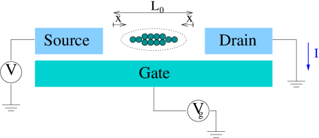
Figure 1: A scheme of the model device studied in this paper. A molecule of average length $L_{0}$ is connected to source and drain electrodes. As it vibrates symmetrically, the distance between the end groups and the electrodes fluctuates thus modulating the tunnelling barrier between the elements. There is also a modulation of the position of the molecular energy levels with respect to the Fermi level not represented in the scheme.

The Hamiltonian of the combined system consists of three terms that describe the isolated molecule, the isolated electrodes, and the coupling between them, respectively,

$$H=H_{M}+H_{E}+H_{M-E}\;.$$ (1)

The Hamiltonian of the molecule is

$$H_{M}=\varepsilon_{d}\hat{n}_{d}+Un_{d\uparrow}n_{d\downarrow}-\lambda\;\left(\hat{n}_{d}-1\right)\left(a+a^{\dagger}\right)+\omega_{0}a^{\dagger}a\;,$$ (2)

where $\hat{n}_{d}=\sum_{\sigma}d^{\dagger}_{\sigma}d_{\sigma}$ is the charge operator and $U$ is the Coulomb repulsion between two electrons on the same molecular orbital. In appropriate units we write the elongation of the molecule as $x=a+a^{\dagger}$, where $a$ and $a^{\dagger}$ are the phonon operators.

The Hamiltonian of the leads is

$$H_{E} = \sum_{{\bf k},\sigma,\ell}\varepsilon_{\ell}({\bf k})\;c^{\dagger}_{{\bf k}\sigma\ell}c_{{\bf k}\sigma\ell}\;\left(\ell={\rm L,R}\right)\;,$$ (3)

where we consider for simplicity the case of identical electrodes with dispersion $\varepsilon_{\textsc{r}}({\bf k})=\varepsilon_{\textsc{l}}({\bf k})=\varepsilon({\bf k})$. We assume for convenience that the conduction band is symmetric with respect to the chemical potential and we take the latter as the origin of energies.

The third term in Eq. (1) is the tunnelling Hamiltonian between the molecule and the electrodes,

$$H_{M-E} = [1+g\;(a+a^{\dagger})]V\sum_{{\bf k},\sigma,\ell}\;\left(d^{\dagger}_{\sigma}\;c_{{\bf k}\sigma\ell}+{\textsc{h.c}}\right)$$

$$\equiv \left[1+g\;(a+a^{\dagger})\right]V\hat{v}\;,$$

where we assumed that the tunnelling matrix element $V$ is $\bf{k}$-independent and we defined the operator $\hat{v}$ for notational convenience.

Note that if either $g=0$ or $\lambda=0$ and $\epsilon_{d}=-U/2$, the Hamiltonian of the model is symmetric under an electron-hole transformation (plus the inversion $x\to-x$ if $\lambda\neq 0$). At the symmetric point, the average number of electrons of the molecule is $n_{d}\equiv\langle\hat{n}_{d}\rangle=1$. If both $g$ and $\lambda$ are non vanishing, this symmetry is lost. We shall see below that this has important consequences.

An expression for the conductance $G$ of the molecular junction at zero bias can be derived using standard methods. Meir and Wingreen (1992); Jauho et al. (1994) We find

$$G=\left.{dI\over dV}\right|_{V=0}={2e^{2}\over h}\ \pi\Delta\int_{-\infty}^{\infty}d\omega\left(-{\partial f(\omega)\over\partial\omega}\right)\widetilde{\rho}_{dd}({\omega})\;,$$ (5)

where $f(\omega)$ is the Fermi function, $\Delta=2\pi\rho_{0}V^{2}$ and $\rho_{0}$ is the electronic density of states of the electrodes evaluated at the Fermi level. The spectral density $\widetilde{\rho}_{dd}(\omega)=-\pi^{-1}{\rm Im}\widetilde{G}_{dd}(\omega)$, where we defined a modified $d$-electron Green function $\widetilde{G}_{dd}(\omega)$ as

$$\widetilde{G}_{dd}(\omega) = -i\int_{0}^{\infty}dte^{i\omega t}\Big{\langle}\left[\left(1+g\;x(t)\right)d_{\sigma}(t),\right.$$ (6)

$$\left.\left(1+g\;x\right)d^{\dagger}_{\sigma}\right]_{+}\Big{\rangle}\;.$$

III Analytical results

III.1 Exact results at zero temperature

The ground state of Hamiltonian (1) is expected to be a Fermi liquid. Exact relationships can then be established between the zero-temperature conductance through the junction, the spectral density of the molecule at the Fermi level and its charge. To derive these relations the structure of the expansion of the electronic Green functions in powers of the electron-electron and electron-phonon interactions coupling constants must be examined.

We start by noting that when the molecule is coupled to the contacts it will in general deform. It is convenient to carry out the perturbation expansion around the deformed ground state. We thus apply a canonical transformation that shifts the phonon operators, $a\to b+\alpha$, and write

$$H(a,a^{\dagger})=H(b+\alpha,b^{\dagger}+\alpha)\equiv H_{\alpha}^{\prime}(b,b^{\dagger})\;,$$ (7)

which defines the transformed Hamiltonian $H_{\alpha}^{\prime}(b,b^{\dagger})$.

Since the ground state energy is invariant under this transformation,

$$E_{0}\equiv\langle H\rangle=\langle H_{\alpha}^{\prime}\rangle\;,$$ (8)

we may take the derivative with respect to $\alpha$ of this equation to obtain,

$$\omega_{0}\;\langle b+b^{\dagger}\rangle_{\alpha}+2\alpha\omega_{0}-2\lambda\langle\hat{n}_{d}-1\rangle_{\alpha}+2gV\langle\hat{v}\rangle_{\alpha}\equiv 0\;,$$ (9)

where $\langle\cdots\rangle_{\alpha}$ denotes an expectation value with respect to the exact ground state of the transformed Hamiltonian. The deformation $\langle x\rangle$ of the molecule is found by imposing that $\langle b+b^{\dagger}\rangle_{\alpha}=0$ on the transformed ground state:

$$\alpha=\frac{\langle x\rangle}{2}=\frac{\lambda}{\omega_{0}}\langle\hat{n}_{d}-1\rangle_{\alpha}-\frac{g}{\omega_{0}}V\langle\hat{v}\rangle_{\alpha}\;.$$ (10)

The transformed Hamiltonian can be expressed as a sum of one-body and many-body terms as

$$H^{\prime} = H^{\prime}_{0}+H^{\prime}_{1}\;,$$ (11)

$$H^{\prime}_{0} = H_{E}+\omega_{0}\;b^{\dagger}b+\widetilde{\varepsilon}_{d}\;\hat{n}_{d}+\widetilde{V}\;\hat{v}\;,$$ (12)

$$H^{\prime}_{1} = \left(b+b^{\dagger}\right)\left[gV\left(\hat{v}-\langle\hat{v}\rangle_{\alpha}\right)-\lambda\left(\hat{n}_{d}-\langle\hat{n}_{d}\rangle_{\alpha}\right)\right]$$

$$+ Un_{d\uparrow}n_{d\downarrow}\;,$$

where we dropped a constant energy shift and we defined the renormalized parameters

$$\widetilde{\varepsilon}_{d}=\varepsilon_{d}-2\lambda\alpha\;,\;\textrm{and}\;\;\widetilde{V}=V\left(1+2g\alpha\right)\;.$$ (14)

The molecule is only coupled to a local symmetric linear combination of the states of the leads,

$$\left|\Psi_{c}\rangle\right.={\cal N}^{-1/2}\sum_{\bf k}\frac{\left|\Psi_{\bf{k},\rm{R}}\rangle\right.+\left|\Psi_{\bf{k},\rm{L}}\rangle\right.}{\sqrt{2}}\;,$$ (15)

where ${\cal N}$ is a normalization factor. The remaining conduction-electron states can be integrated out reducing the problem to an effective interacting two-site model with a damping term that reflects the coupling of the subsystem to the electrodes. Physical quantities may be obtained from the $2\times 2$ Green-function matrix

$${\bf G}(\omega)=\left(\begin{array}[]{cc}G_{cc}(\omega)&G_{cd}(\omega)\\ \\ G_{dc}(\omega)&G_{dd}(\omega)\end{array}\right)\;.$$ (19)

The Green function associated to the one-body Hamiltonian $H^{\prime}_{0}$ is

$${\bf G}_{0}(\omega)=\left(\begin{array}[]{cc}1/G^{0}_{cc}(\omega)&-\sqrt{2}\;\widetilde{V}\\ \\ -\sqrt{2}\;\widetilde{V}&\omega-\widetilde{{\epsilon}}_{d}\end{array}\right)^{-1}\;,$$ (23)

where, in the wideband limit, $G^{0}_{cc}(\omega)=\sum_{\bf{k}}1/(\omega-\varepsilon_{\bf k})=-i\pi\rho_{0}$ and $\rho_{0}$ is the bulk density of states of the electrodes. Note that ${\bf G}_{0}(\omega)$ is not the non-interacting Green function and it includes effects of the interactions to all orders through the renormalized parameters (14).

The remaining effects of the interaction $H^{\prime}_{1}$ are embodied in a self-energy matrix defined through the Dyson equation

$${\bf G}^{-1}(\omega)={\bf G}_{0}^{-1}(\omega)-{\bf\Sigma}(\omega)\;.$$ (24)

In a Fermi-liquid ground state all the elements of the self-energy matrix are purely real at the Fermi level. We checked that this is the case for our model by computing a few low-order diagrams in the expansion of ${\bf{\Sigma}}$ in powers of $H^{\prime}_{1}$. Luttinger’s theorem Abrikosov et al. (1963); Hewson (1997)can then be generalized to the present situation in order to establish some useful Fermi-liquid relationships.

We found a simple relationship between $\rho_{cc}(0)$, the $c$-component of the spectral density at the Fermi level, and the electronic population of the molecule in the physically relevant wideband limit. It reads,

$$\rho_{cc}(0)=\rho_{0}\cos^{2}\left(\frac{\pi}{2}n_{d}\right)\;.$$ (25)

Equation (25) is an exact result valid for all values of the parameters of the Hamiltonian (1). For $g=0$ but keeping $\lambda$ arbitrary we found an equivalent expression for $\rho_{dd}(0)$, the projection of the spectral density on the molecular orbital. In the wideband limit this is

$$\left.\rho_{dd}(0)\right|_{g=0}=\frac{1}{\pi\Delta}\sin^{2}\left(\frac{\pi}{2}n_{d}\right)\;,$$ (26)

The content of Eq. (26) is that, for $g=0$, the $d$-spectral density of the interacting system at the Fermi level is pinned at the value it takes for a non-interacting system with the same electron occupancy. This is a well known result for model (1) in the absence of electron-phonon coupling. Hewson (1997) We see that it remains valid for all values of $\lambda$ and $g=0$.

However, Luttinger’s theorem does not lead to a similar result for $\rho_{dd}$ in the general $g\neq 0$ case and the elements of the self-energy matrix appear explicitly in the corresponding expression.

There is some simplification in the particular case $\lambda=0$, $\epsilon_{d}=-U/2$. Then, the Hamiltonian (1) is electron hole symmetric [c.f. Section II], $n_{d}=1$, and $\Sigma_{cc}(0)$ and $\Sigma_{dd}(0)$ vanish. In this case we find

$$\left.\rho_{dd}(0)\right|_{\lambda=0,n_{d}=1}=\frac{1}{\pi\widetilde{\Delta}}$$ (27)

where

$$\widetilde{\Delta}=\pi\rho_{0}\left[\sqrt{2}\;\widetilde{V}+\Sigma_{cf}(0)\right]^{2}\;.$$ (28)

It can be easily shown that $\Sigma_{cf}$ is of order $g^{2}$ and higher. It then follows from Eqs. (10), (14) and (28) that $\widetilde{\Delta}=\Delta\left(1+{\cal{O}}(g^{2})+\cdots\right)$.

Interestingly, the non-universality of $\rho_{dd}(0)$ (of which Eq. (27) is only an example) does not extend to the $T=0$ conductance. The latter is obtained setting $T=0$ in Eq. (5).

$$\frac{G}{G_{0}}=\pi\Delta\;\widetilde{\rho}_{dd}(0)\;,$$ (29)

where $G_{0}=2e^{2}/h$ is the quantum of conductance.

An expression for the modified Green function $\widetilde{G}_{dd}(\omega)$ can be obtained by writing down the equation of motion for the conduction-electron Green function $G_{cc}(\omega)$ using the definition (6) and the original Hamiltonian (1). We find

$$G_{cc}(\omega)=G^{0}_{cc}(\omega)+2V^{2}G^{0}_{cc}(\omega)\widetilde{G}_{dd}(\omega)G^{0}_{cc}(\omega)\;.$$ (30)

Setting $\omega=0$ and taking the imaginary part of the above equation this becomes

$$\rho_{cc}(0)=\rho_{0}\left[1-\pi\Delta\widetilde{\rho}_{dd}(0)\right]\;.$$ (31)

Comparing Eq. (31) with the Fermi-liquid relationship (25) we find

$$\pi\Delta\widetilde{\rho}_{dd}(0)\equiv\frac{G}{G_{0}}=\sin^{2}\left(\frac{\pi}{2}n_{d}\right)\;.$$ (32)

The zero-temperature conductance thus depends only on the occupation of the molecular orbital just as in the absence of tunnelling barrier modulation and it reaches its maximum value $G_{0}$ when $n_{d}=1$. A related result was obtained in Ref. Mitra et al., 2004 in perturbation theory in $\lambda$ for $U=0$ and $g=0$.

III.2 Analysis of limiting cases

Many features of the solution of our problem can be found from an analysis of the limiting cases of small and large electron-phonon coupling.

We start from the Hamiltonian of the isolated molecule given in Eq. (2). Its eigenvalues and eigenfunctions can be written down explicitly:Cornaglia et al. (2004)

$$\begin{array}[]{ll}\left|0,m\right>=\widetilde{U}^{+}\left|0\right>_{e}\left|m\right>,&E_{0,m}=-{\lambda^{2}\over\omega_{0}}+m\omega_{0},\\ \\ \left|\sigma,m\right>=\left|\sigma\right>_{e}\left|m\right>,&E_{\sigma,m}=\varepsilon_{d}+m\omega_{0},\\ \\ \left|2,m\right>=\widetilde{U}^{-}\left|\uparrow\downarrow\right>_{e}\left|m\right>,&E_{2,m}=-{\lambda^{2}\over\omega_{0}}+2\varepsilon_{d}+U+m\omega_{0},\end{array}$$ (38)

where the subscript $e$ denotes electronic states, $\left|m\right>$ is $m$-th excited state of the harmonic oscillator and

$$\widetilde{U}^{\pm}=\exp{\left[\pm{\frac{\lambda}{\omega_{0}}}\left(a-a^{\dagger}\right)\right]}\;.$$ (39)

At $\varepsilon_{d}=-U/2$ the states with zero and two electrons are degenerate. We take this as a reference point and write

$$\varepsilon_{d}=-\frac{U}{2}+V_{d}\;.$$ (40)

The number of electrons in the ground state of the molecule is either odd or even depending on whether $2\lambda^{2}/\omega_{0}$ is smaller or larger than $U$. It is convenient to define an effective interaction parameter,

$$U_{\textrm{eff}}=U-\frac{2\lambda^{2}}{\omega_{0}}$$ (41)

It will be seen below that the physics in the cases $U_{\textrm{eff}}>0$ and $U_{\textrm{eff}}<0$ is quite different.

III.2.1 $U_{\textrm{eff}}>0$

In this case the ground-state of the isolated molecule for $|V_{d}|<U/2$ is the spin-doublet $\left|\sigma,0\right>$. There is a charge excitation gap given by $\sim U_{\rm eff}=U-2\lambda^{2}/\omega_{0}$ for $V_{d}=0$ and a phonon gap $\omega_{0}$. The low-energy excitations are spin fluctuations.

An effective Hamiltonian for excitations involving the spin doublet can be derived by perturbatively projecting out the empty and doubly occupied states from the space of available states by means of a Schrieffer-Wolff transformation. To lowest order in $V/U$, the low-energy effective Hamiltonian for spin fluctuations $H_{\rm eff}$ is

$$H_{\rm{eff}}=\omega_{0}a^{\dagger}a+H_{E}+J{\bf{S}}\cdot{\bf{s}}_{c}\;,$$ (42)

where $\bf{S}$ is the spin operator for the doublet and ${\bf{s}}_{c}=1/2\;\sum_{s,s^{\prime}}\;c^{\dagger}_{s}\;{\mathchar 28955\relax}_{s,s^{\prime}}\;c{}_{s^{\prime}}$ is the spin operator of an electron on the state (15) coupled to the molecule. The coupling constant $J$ is given by

$$J=\frac{J_{0}}{2}\;\sum_{m=0}^{\infty}~{}\sum_{\mu=\pm}{|\langle 0|[1+g(a+a^{\dagger})]\widetilde{U}^{\mu}|m\rangle|^{2}\over 1-2\lambda^{2}/\omega_{0}U+2m\omega_{0}/U},$$ (43)

where $J_{0}=8\Delta/(\pi U\rho_{0})$ and we have taken $V_{d}=0$ for simplicity.

A simple analytical expression can be derived in the limit of small electron-phonon coupling, $g,\lambda/U\ll 1$. We find

$$J=J_{0}\left[1+{\left(2\lambda/U\right)^{2}+g^{2}\over 1+2\omega_{0}/U}+\cdots\right]\;\;.$$ (44)

Therefore, $J$ increases with the electron-phonon coupling in the weak coupling limit.

Equation (42) is the well known Kondo model Hamiltonian . Hewson (1997) The dependence of the conductance on temperature, gate-voltage and magnetic field is well understood in the absence of electron phonon coupling. We summarize below the main features for $g=\lambda=0$.

At $T=0$, there is a narrow resonance of width $T_{K}\sim D\exp\left(-1/(J\rho_{0})\right)$ in the $d$-electron spectral density at the Fermi level. This resonance provides a channel for conduction and, at the symmetric point, $n_{d}=1$, $G=G_{0}$ in agreement with Luttinger’s theorem.

For $V_{d}\neq 0$, the gap between the ground state doublet and the empty state ($V_{d}>0$), or the doubly occupied state ($V_{d}<0$) is reduced. The charge then deviates from $n_{d}=1$. The Kondo resonance shifts with respect to the Fermi level and the $\rho_{dd}(0)$ decreases. For $|V_{d}|\gtrsim U/2$ the Kondo resonance disappears. There is thus a peak in $G(V_{g})$ whose width $\sim U$ is large. An applied magnetic field $B$ also destroys the Kondo resonance by breaking the symmetry between the spin up and spin down ground states. This happens for $B\sim T_{K}$ which is very small in the Kondo limit. Therefore, the peak in $G(B)$ is narrow. At finite temperature the conductance at the symmetric point decreases becoming very small for $T\gtrsim T_{K}$. In this temperature range $G$ exhibits Coulomb blockade peaks at gate voltages $V_{d}\sim\pm U/2$.

These features are present throughout the weak coupling regime with some minor modifications. It follows from equation (44) that $T_{K}$ increases with increasing $\lambda$ and $g$. Therefore, the peak in $G(B)$ becomes wider and the temperature variation of the conductance at resonance becomes slower. If both $g$ and $\lambda\neq 0$ the zero-temperature peak in $G(V_{d})$ shifts from $V_{d}=0$ to $V_{d}=V^{\star}_{d}$ such that $n_{d}=1$ and acquires an asymmetric shape. These features are related to the loss of particle-hole symmetry referred to above. The conductance is higher to the left of the maximum than to its right because for negative values of $V_{d}-V^{\star}_{d}$ the doubly occupied state that has a stronger coupling to the electrodes is favored. The width of the peak and the separation between the finite-temperature Coulomb blockade peaks, that are also asymmetric, decrease with increasing $\lambda$ mirroring the evolution of $U_{\textrm{eff}}$.

III.2.2 $U_{\textrm{eff}}<0$

In this regime the ground-state for $V_{d}=0$ is a charge doublet formed by the states $\left|2,0\right>$ and $\left|0,0\right>$. The low-energy excitations of the system are thus charge fluctuations and there is a large gap $\sim 2\lambda^{2}/\omega_{0}-U$ for spin excitations.

We discuss the case $g=0$ first. A low-energy effective Hamiltonian can be found as before applying a Schrieffer-Wolff transformation, but now we project out the singly occupied states. We introduce pseudo-spin operators $\tau^{z}_{d}$ and $\tau^{z}_{c}$ with eigenvalues $\pm 1/2$, corresponding to the eigenvalues $Q=2$ and $Q=0$ of the charge of the molecule and of the orbital $c$, respectively. We also define raising and lowering operators , $\tau^{+}_{d}=\left(\tau^{-}_{d}\right)^{\dagger}=d^{\dagger}_{\uparrow}d^{\dagger}_{\downarrow}$ and similar ones for the leads. In terms of these, the effective Hamiltonian for $V_{d}=g=0$ is:

$$H=H_{E}+J_{\parallel}\;\tau^{z}_{d}\;\tau^{z}_{c}+\frac{J_{\perp}}{2}\left(\tau^{+}_{d}\;\tau^{-}_{c}+\tau^{-}_{d}\;\tau^{+}_{c}\right)\;,$$ (45)

with the couplings

$$J_{\parallel} = J_{0}\sum_{m=0}^{\infty}{\langle 0|\widetilde{U}^{+}|m\rangle\langle m|\widetilde{U}^{-}|0\rangle\over{2\lambda^{2}/\omega_{0}U}-1+{2m\omega_{0}/U}}\;,$$ (46)

$$J_{\perp} = J_{0}\sum_{m=0}^{\infty}{\langle 0|\widetilde{U}^{+}|m\rangle\langle m|\widetilde{U}^{+}|0\rangle\over{2\lambda^{2}/\omega_{0}U}-1+{2m\omega_{0}/U}}\;.$$ (47)

Equations (45)-(47) define the Hamiltonian of an anisotropic Kondo model (AKM).Costi and Kieffer (1996); Costi (1998) The couplings (46) and (47) can be easily estimated in the limit $\lambda/\omega_{0}\gg 1$ by noting that

$$\langle 0|\widetilde{U}^{+}|m\rangle\langle m|\widetilde{U}^{-}|0\rangle = e^{-\left(\lambda/\omega_{0}\right)^{2}}\;\frac{\left(\lambda/\omega_{0}\right)^{2m}}{m!}$$

$$= (-1)^{m}\langle 0|\widetilde{U}^{+}|m\rangle\langle m|\widetilde{U}^{+}|0\rangle\;.$$

Considered as a function of $m$, the last expression on the right hand side of the upper line of Eq. (III.2.2) is strongly peaked at $m^{\star}=(\lambda/\omega_{0})^{2}\gg 1$, while the denominators in Eqs (46) and (47) are slowly varying functions of $m$. In the strong coupling limit these can be approximated by their value at $m^{\star}$ and taken out of the sum. This results in

$$J_{\parallel}\sim\frac{4J_{0}\omega_{0}U}{\lambda^{2}}\;,\;\;\;J_{\perp}\sim J_{\parallel}e^{-2\left(\lambda/\omega_{0}\right)^{2}}\;.$$ (49)

This strong anisotropy originates in the fact that the phonon ground states corresponding to the two charge states $Q_{d}=2$ and $Q_{d}=0$ are very different. In the strong-coupling limit, the anisotropy ratio $J_{\perp}/J_{\parallel}$ is precisely the overlap $\langle 2,0|0,0\rangle$ between them [c.f. Eq. (38)]. The Kondo temperature of the AKM is Costi and Kieffer (1996); Costi (1998)

$$T_{{\textsc{akm}}}\sim\left({J_{\perp}\over J_{\parallel}}\right)^{1\over J_{\parallel}\rho_{0}}\sim D\exp\left[-{\pi\omega_{0}\over\Delta}\left({\lambda\over\omega_{0}}\right)^{4}\right]\;,$$ (50)

where the last expression is its asymptotic form for large $\lambda/\omega_{0}$.

In contrast with the weak-coupling situation, $T_{\textsc{akm}}$ decreases sharply when $\lambda$ increases. Application of a small potential $|V_{d}|\gtrsim T_{\textsc{akm}}$ splits the charge doublet and destroys the Kondo resonance. Hence, the peak in $G(V_{d})$ is very narrow in this limit. Conversely, the doublet is insensitive to a magnetic field and the width $\sim 2\lambda^{2}/\omega_{0}-U$ of the peak in $G(B)$ is now large. Finally, no Coulomb blockade peaks are to be seen upon application of a gate voltage because it leads to an increase of the energy difference between a ground state with zero or two electrons and an excited state with one electron irrespective of its sign. These features are opposite of those that characterize the properties of $G$ in the weak coupling regime.

We discuss now the case $g\neq 0$. The modulation of the tunnelling amplitude has two effects. The first one is to renormalize the coupling constants,

$$J_{\parallel}\; \rightarrow \;J^{\prime}_{\parallel}=J_{\parallel}\;[1+(g\lambda/\omega_{0})^{2}]\;,$$

$$\;\;\;J_{\perp}\; \rightarrow \;J^{\prime}_{\perp}=J_{\perp}\;[1-(g\lambda/\omega_{0})^{2}]\;.$$

The second effect is the appearance of a term in the Hamiltonian that breaks the symmetry between the two charge states, favoring the doubly occupied one:

$$H_{\textsc{akm}}\;\rightarrow\;H^{\prime}_{\textsc{akm}}-\frac{g\lambda}{\omega_{0}}\;J_{\parallel}\tau^{z}_{d}\;,$$ (52)

where $H^{\prime}_{\textsc{akm}}$ denotes the AKM Hamiltonian with the new couplings. These effects can be understood quite easily. In the state with charge $Q_{d}=2$ the molecule elongates. This increases its coupling to the electrodes and its energy is lowered with respect to that of the empty state. The tunnelling barrier between them also increases which translates into a reduction of $J_{\perp}$.

We can use the modified couplings (LABEL:eq:effect-of-g-oncouplings) to compute the $g$-dependent Kondo temperature. The result is,

$${T^{\prime}_{\textsc{akm}}\over T_{\textsc{akm}}}\sim\exp\left[{\pi g^{2}\omega_{0}\over\Delta}\left({\lambda\over\omega_{0}}\right)^{4}\;\left(\left(\lambda\over\omega_{0}\right)^{2}-1\right)\right]\;.$$ (53)

In the strong coupling regime the Kondo temperature increases or decreases with $g$, depending on the ratio $\lambda/\omega_{0}$.

The consequences of a finite $g$ on the conductance are twofold. First, the peak in $G(V_{d})$ no longer occurs at $V_{d}=0$ but it shifts to $V^{\star}_{d}\sim g\;J_{\parallel}\;\lambda/\omega_{0}$, the value for which the asymmetry generated by the second term in Eq. (52) is compensated. Secondly, as in the previous case, the singly occupied states are more strongly coupled to the doubly occupied state leading to asymmetry in the shape of $G(V_{d})$. This time, the asymmetry is much more pronounced than for weak coupling because the relative weights of the components of with $Q_{d}=0$ and $Q_{d}=2$ in the wavefunction are more sensitive to $V_{d}$.

IV Numerical results

In this Section we present the numerical solution of model (1) using the numerical renormalization group method (NRG) Wilson (1975); Krishna-murthy et al. (1980); Costi et al. (1994); Hewson and Meyer (2002) incorporating a modification designed to improve the accuracy of the computation of the spectral density. Hofstetter (2000)

Results for the case $g=0$ were discussed in a previous paper. Cornaglia et al. (2004) Here, we focus on the effects of tunnelling barrier modulation on the conductance.

In our numerical calculations we used half the bandwidth of the conduction electron band $D$ as the unit of energy. The parameters $U=0.1$, $\Delta=0.01$, and $\omega_{0}=0.05$ were kept fixed and we studied the conductance as a function of $g$, $\lambda$ and $V_{d}$.

IV.1 The electron hole symmetric case at $\lambda=0$

We start by analyzing the electron-hole symmetric case, $\lambda=0$, $V_{d}=0$ [c.f. Eq. (40)]. Fig. 2 shows the spectral density $\rho_{dd}(\omega)$ at zero temperature for several values of $g$ between 0 and 0.5.

The top curve corresponds to $g=0$. It exhibits a narrow Kondo resonance centered at the Fermi level and two Coulomb peaks at $\omega\sim\pm U/2$. The height of the Kondo resonance is $1/\pi\Delta\sim 32$ in this case.

With increasing $g$ the hight of the central peak decreases and its width increases. This evolution is shown in more detail in the left inset to the figure.

That the height of the central peak depends upon $g$ shows that $\rho_{dd}(0)$ does not obey Luttinger’s theorem in the simple form of Eq. (26). An effective hybridization parameter $\widetilde{\Delta}$ may be obtained from the numerical values of $\rho_{dd}(0)$ using Eq. (27). Its dependence on $g$ is represented in the right inset to the figure. It is seen that $\widetilde{\Delta}$ increases quadratically with $g$ in the electron-hole symmetric case as was anticipated in Section III.1.

The figure shows that the width $\Gamma$ of the Kondo resonance increases monotonically with $g$. The dependence of $\Gamma$ on $g$ is represented in the inset to Fig. 3 that shows that $\log\Gamma$ varies quadratically with $g$ for small $g$. This behavior can be understood from Eq. (44), that predicts a quadratic increase of the Kondo coupling $J$ for small $g$ and $\lambda=0$, recalling that $\Gamma\sim T_{K}$ and that the latter varies exponentially with $J^{-1}$.

Finally, we observe that the Coulomb peaks broaden with increasing $g$ until they eventually disappear when the system enters the mixed-valence regime for large $g$.

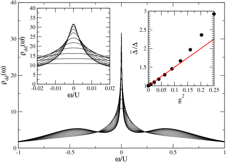
Figure 2: Spectral density $\rho_{dd}(\omega)$ at zero temperature in the electron-hole symmetric case. The electron-phonon coupling $g$ varies between 0 and 0.5 in steps of 0.05 from top to bottom in the region of the central peak. Left inset: a zoom of the central part of the main figure. Right inset: $g$-dependence of the effective hybridization parameter $\widetilde{\Delta}$.

The temperature dependence of the conductance at $V_{d}=0$ is shown in Fig. 3 for the same values of $g$ as in Fig. 2. $G(g,T)$ reaches its maximum value $G_{0}$ at $T=0$ for all $g$ in agreement with Eq. (32). This confirms the result of Fermi-liquid theory that tunnelling barrier modulation does not lead to a renormalization of the value of the conductance at resonance despite that the spectral density at the Fermi level is modified.

The conductance at resonance decreases with temperature. The temperature scale for this process is the Kondo temperature. The observed shift of the curves to higher temperatures with increasing $g$ reflects the evolution of the latter.

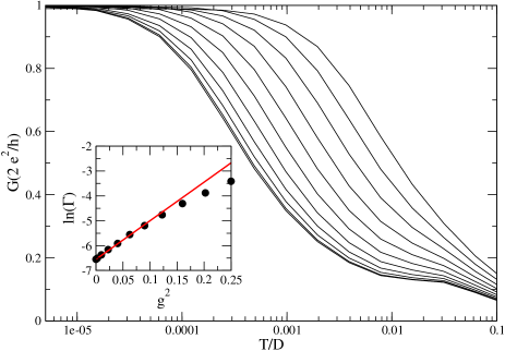
Figure 3: Temperature dependence of the conductance in the electron-hole symmetric case. The electron phonon couplings are as in Fig. 2. The curves correspond to increasing values of $g$ from left to right. Inset: $g$-dependence of the width of the central peak of the curves shown in the previous figure

IV.2 The general case, $\lambda$ and $g\neq 0$

We pointed out in Section II that when both $\lambda$ and $g$ are non zero the system looses electron-hole symmetry. This is at the origin of several observable features in the frequency dependence of the molecule’s spectral density and in the dependence of the conductance on gate voltage. All the results described below were obtained with $g=0.2$.

Figure 4 shows the $d$-electron spectral density at zero temperature in the strong coupling regime, $U_{\textrm{eff}}<0$. We display results for three values of $V_{d}$: $V_{d}^{\star}$, chosen so that $n_{d}=1$, and $V_{d}=V^{\star}_{d}\pm\delta V_{d}$.

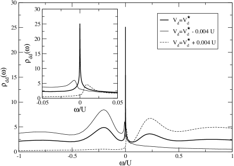
Figure 4: Spectral density $\rho_{dd}(\omega)$ at $T=0$ for $\lambda=-0.06$ and $g=0.2$. Thick line: $V_{d}/U=V_{d}^{\star}/U=0.159$, $n_{d}=1$. Dashed line: $V_{d}/U=0.163$, $n_{d}<1$. Thin line: $V_{d}/U=0.155$, $n_{d}>1$. Inset: a zoom of the central peak showing the evolution of the Kondo peak with varying $V_{d}$.

The thick line represents $\rho_{dd}(\omega)$ for $V_{d}=V_{d}^{\star}$. We observe a very narrow peak at the Fermi level due to the anisotropic Kondo effect described in Section III.2.2. We also observe sideband peaks that are associated to excitation of the higher levels of the isolated molecule at $\omega\sim\pm U_{\textrm{eff}}$ [c.f. Eq. 38]. It is seen that these are not positioned symmetrically with respect to the central peak and that their widths and heights are different. As discussed above, the origin of the asymmetry is that the states with $Q_{d}=0$ and $Q_{d}=2$ are coupled with different strength to the states with $Q_{d}=1$. The matrix element for the transition $|2,0\rangle\rightarrow|1\sigma,0\rangle$ is larger than that for the transition $|0,0\rangle\rightarrow|1\sigma,0\rangle$.

The spectral densities for $V_{d}=V^{\star}_{d}\pm\delta V_{d}$ are represented in the figure by dashed and solid thin lines, respectively. For our choice of parameters, $|\delta V_{d}|\lesssim T_{\textsc{akm}}$. Therefore, the Kondo resonance continues to exist but it shifts and its amplitude decreases as shown in the inset to Fig. 4 which is a detailed view of the central part of the main plot.

When $V_{d}>V_{d}^{\star}$ the empty orbital has a larger weight in the ground state wavefunction than the doubly occupied orbital. Then, the sideband at $\omega>0$ is enhanced and that at $\omega>0$ is suppressed. The opposite occurs for $V_{d}<V_{d}^{\star}$.

For $|\delta V_{d}|\gtrsim T_{\textsc{akm}}$ (not shown), the molecule becomes fully charge-polarized Cornaglia et al. (2004) and the Kondo peak is completely suppressed.

We have also computed the spectral density in the weak coupling regime, $U_{\textrm{eff}}>0$ (not shown). For moderate values of $g$, $V_{d}^{\star}\sim 0$ and the effects of the asymmetry are much less pronounced than for the strong coupling case just discussed.

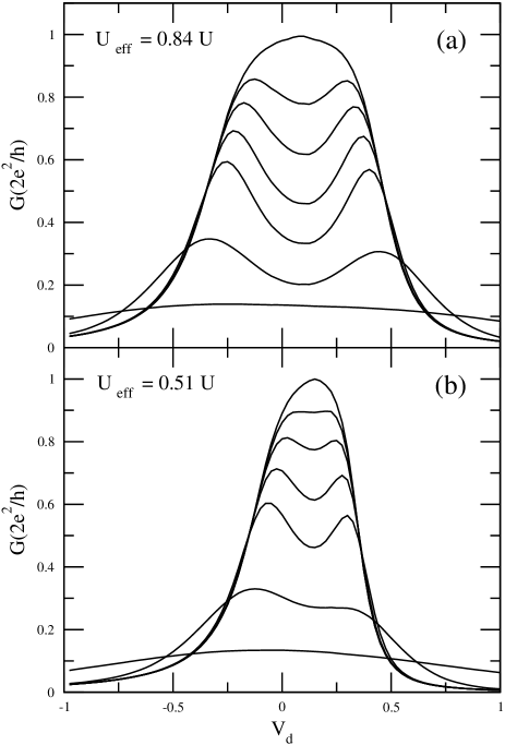
Figure 5: Conductance as a function of $V_{d}$ and temperature for weak coupling, $U_{\textrm{eff}}>0$. Panel (a): $\lambda=0.02$. Panel (b): $\lambda=0.035$. Temperatures are: $T=0,7.3\times 10^{-4},1.5\times 10^{-3},3\times 10^{-3},6\times 10^{-3},0.023$ and 0.094 from top to bottom. In all cases $g=0.2$.

We now turn to the analysis of the results for the conductance. Fig. 5 shows $G(V_{d})$ for several temperatures and two values of $\lambda$, both in the regime $U_{\textrm{eff}}>0$. We observe a broad conductance peak of width $\sim U_{\textrm{eff}}$ at zero temperature. There is perfect conductance at $V^{\star}_{d}\neq 0$ and the peak is asymmetric with respect to $V_{d}^{\star}$.

At finite temperature the Kondo effect is first suppressed at the center of the peak where the Kondo temperature is the lowest, leading to a two-peak structure. There are two Coulomb blockade peaks whose widths and hights are different for the same reasons that make the spectral density asymmetric.

A comparison between Figs. 5(a) and 5(b) shows that an increase of $\lambda$ leads to an enhancement of the anisotropy. This is easily understood as we saw that the latter arises from the simultaneous presence of ELM and TBM. We also observe a narrowing of the Coulomb blockade valley that originates from the decrease of $U_{\textrm{eff}}$.

A further increase of $\lambda$ takes the molecule away from the standard Coulomb blockade regime. Fig. 6 shows results for $U_{\textrm{eff}}=0$. Here, the differences between the energies of the four charge states of the isolate molecule are comparable with their width and no Kondo effect is expected to occur. No Coulomb blockade peaks appear upon raising the temperature as we argued in Section III.2.2.

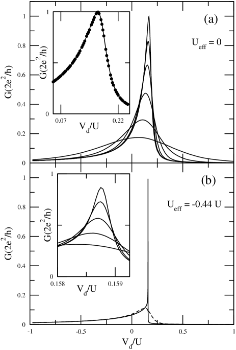
Figure 6: Panel (a): Conductance as a function of $V_{d}$ and temperature for $U_{\textrm{eff}}=0$ ($\lambda=0.05$). Temperatures are $T=0,3\times 10^{-3},6\times 10^{-3},1.2\times 10^{-2},2.4\times 10^{-2}$ and $4.7\times 10^{-2}$. Inset: Check of the validity of Luttinger’s theorem, Eq. (32). Panel (b) Same as (a) for $U_{\textrm{eff}}<0$ ($\lambda=0.06$). Temperatures are $T$=0 and 0.012. Inset. Zoom of the conductance peak for temperatures $T=1.1\times 10^{-5},2.3\times 10^{-5},4.6\times 10^{-5},9.2\times 10^{-5}$ and $1.83\times 10^{-4}$ from top to bottom. For all the curves shown in this figure $g=0.2$.

The conductance in the strong-coupling case $U_{\textrm{eff}}<0$ is shown in Fig. 6(b). As in the previous regimes the zero-temperature conductance is enhanced and reaches the quantum of conductance at some value of $V_{d}$ but, now, the peak is exceedingly narrow. This is the regime where the anisotropic Kondo effect occurs. The width of the peak in $G(V_{d})$ is now $T_{\textsc{akm}}$ not $|U_{\textrm{eff}}|$. A very small shift $|\delta V_{d}|\gtrsim T_{\textsc{akm}}$ is sufficient to destroy the Kondo resonance. The asymmetry generated by the tunnelling barrier is in this case extremely pronounced because the charge on the molecule switches from $n_{d}=0$ and $n_{d}=2$ within a very small interval of values of $V_{d}$. Similarly, the conductance at resonance decreases very rapidly with increasing temperature as shown in the inset to Fig. 6(b).

We close this Section with a comparison between the conductance of the device calculated from Eq. (5) and that computed from Eq. (32), using $n_{d}(V_{d})$ obtained from the NRG calculation. The data are shown in the inset to Fig. 6(a). It is seen that the Fermi-liquid relation (32) is satisfied within the numerical error.

V Conclusions

We studied the linear transport properties of a model molecular transistor in the presence of electron-electron and electron-phonon interactions analytically and by numerically solving the model using the Numerical Renormalization Group method.

Electron-phonon interactions lead to modulation of the positions of the energy levels of the molecule with respect to the Fermi level and of the height of the tunnelling barrier between the molecule and the electrodes. These effects give rise to new features in the spectral and transport properties of the system.

We found that when there is tunnelling barrier modulation, the strength of the coupling between the molecule and the leads depends on the charge of the former. In general this effect breaks electron-hole symmetry leading to an asymmetric curve of conductance as a function of gate voltage.

The Kondo effect occurs in the presence of electron-phonon interactions but its nature is quite different for weak and strong coupling. In the first regime the ground state of the isolated molecule is a spin doublet and this leads to a standard Kondo effect with renormalized parameters. In the second regime the lowest lying states of the isolated molecule form a charge doublet and the associated charge fluctuations are described by an anisotropic Kondo model in a narrow interval of gate voltages. The two charge states of the doublet are coupled differently to excited states which gives rise to pronounced asymmetries in the conductance and in the spectral density.

We established Fermi-liquid relationships for the interacting model. Tunnelling barrier modulation leads to a non-universal relation between the spectral density of the molecule and the electron occupancy. Quite remarkably, the relation between the zero-temperature conductance and the charge remains unchanged. An important consequence is that there is perfect transmission in all regimes when the number of electrons in the molecule is an odd integer.

References

- Klein et al. (1997) D. L. Klein, R. Roth, A. K. L. Lim, A. P. Alivisatos, and P. L. McEuen, Nature 389, 699 (1997).
- Park et al. (2002) J. Park, A. N. Pasupathy, J. I. Goldsmith, C. Chang, Y. Yaish, J. R. Petta, M. Rinkoski, J. P. Sethna, H. D. Abruña, P. L. McEuen, et al., Nature 417, 722 (2002).
- Kubatkin et al. (2003) S. Kubatkin, A. Danilov, M. Hjort, J. Cornil, J.-L. Brédas, N. Stuhr-Hansen, P. Hedegård, and T. Bjørnholm, Nature 425, 698 (2003).
- Goldhaber-Gordon et al. (1998) D. Goldhaber-Gordon, H. Shtrikman, D. Mahalu, D. Abusch-Magder, U. Meirav, and M. A. Kastner, Nature 391, 156 (1998).
- Liang et al. (2002) W. Liang, M. P. Shores, M. Bockrath, J. R. Long, and H. Park, Nature 417, 725 (2002).
- Yu and Natelson (2004) L. H. Yu and D. Natelson, Nano Letters 4(1), 79 (2004).
- (7) L. H. Yu, Z. K. Keane, J. W. Ciszek, L. Cheng, M. P. Stewart, J. M. Tour, and D. Natelson, cond-nat/0408052.
- Ho (2002) W. Ho, J. Chem. Phys. 55, 11033 (2002).
- Park et al. (2000) H. Park, J. Park, A. K. L. Lim, E. H. Anderson, A. P. Alivisatos, and P. L. McEuen, Nature 407, 57 (2000).
- Weig et al. (2004) E. M. Weig, R. H. Blick, T. Brandes, J. Kirschbaum, W. Wegscheider, M. Bichler, and J. P. Kotthaus, Phys. Rev. Lett. 92, 046804 (2004).
- Mitra et al. (2004) A. Mitra, I. Aleiner, and A. Millis, Phys. Rev. B 69, 245302 (2004).
- M.-T.Kuo and Chang (2002) D. M.-T.Kuo and Y. C. Chang, Phys. Rev. B 66 (2002).
- Flensberg (2003) K. Flensberg, Phys. Rev. B 68, 205323 (2003).
- Cornaglia et al. (2004) P. S. Cornaglia, H. Ness, and D. R. Grempel, To appear in Phys. Rev. Lett. (2004).
- Arrachea et al. (2003) L. Arrachea, A. A. Aligia, and G. E. Santoro, Phys. Rev. B 67, 134307 (2003).
- Meir and Wingreen (1992) Y. Meir and N. S. Wingreen, Phys. Rev. Lett. 68, 2512 (1992).
- Jauho et al. (1994) A.-P. Jauho, N. S. Wingreen, and Y. Meir, Phys. Rev. B 50, 5528 (1994).
- Abrikosov et al. (1963) A. A. Abrikosov, L. P. Gorkov, and I. E. Dzyaloshinski, Methods of Quantum Field Theory in Statistical Physics (Prentice-Hall, Englewood-Cliffs, New Jersey, 1963).
- Hewson (1997) A. C. Hewson, The Kondo Problem to Heavy Fermions (Cambridge University Press, 1997).
- Costi and Kieffer (1996) T. A. Costi and C. Kieffer, Phys. Rev. Lett. 76, 1683 (1996).
- Costi (1998) T. A. Costi, Phys. Rev. Lett. 80, 1038 (1998).
- Wilson (1975) K. G. Wilson, Rev. Mod. Phys. 47, 773 (1975).
- Krishna-murthy et al. (1980) H. R. Krishna-murthy, J. Wilkins, and K. G. Wilson, Phys. Rev. B 21, 1003 (1980).
- Costi et al. (1994) T. A. Costi, A. C. Hewson, and V. Zlatić, J. Phys.:Condens. Matter 6, 2519 (1994).
- Hewson and Meyer (2002) A. C. Hewson and D. Meyer, J. Phys.:Condens. Matter 14, 427 (2002).
- Hofstetter (2000) W. Hofstetter, Phys. Rev. Lett. 85, 1508 (2000).
- Stephan et al. (1997) W. Stephan, M. Capone, M. Grilli, and C. Castellani, Phys. Lett. A 227 (1-2) (1997).