Is small-world network disordered?

Abstract

Recent renormalization group results predict non self averaging behaviour at criticality for relevant disorder. However, we find strong self averaging(SA) behaviour in the critical region of a quenched Ising model on an ensemble of small-world networks, despite the relevance of the random bonds at the pure critical point.

I Self-averaging

Very often in physics one encounters situations where quenched disorder plays a prominent role. Any physical property $X$ of such a disordered system, therefore, requires an averaging over all realisations. It would suffice to have a description in terms of the average $[X]_{\rm av}$ where $[..]_{\rm av}$ denotes averaging over realisations (“sample averaging”) provided the relative variance $R_{X}=V_{X}/[X]^{2}_{\rm av}\to 0$ for large $N$, where $V_{X}=[X^{2}]_{\rm av}-[X]^{2}_{\rm av}$. In such a case a single large system is enough to represent the ensemble. Such a quantity is called self-averaging. Off criticality, if one builds up a large lattice from smaller blocks, then thanks to the additivity property of an extensive quantity, central limit theorem guarantees that $R_{X}\sim N^{-1}$ ensuring self-averaging. In contrast, at a critical point, because of long range correlations the answer to the question as to whether $X$ is self-averaging or not becomes non-trivial.

Randomness at a pure critical point is classified as relevant or irrelevant if, following the standard definition of relevance, it changes the critical behaviour (i.e. the critical exponents) of the pure system. Recent renormalization group and numerical studies have shown that if randomness or disorder is relevant, then self-averaging property is lostAH-PRL-96 ; WD-PRE-98 . In particular, $R_{X}$ at the critical point approaches a constant as $N\to\infty$. Such systems are called non self-averaging. A serious consequence of this is that unlike the self-averaging case, even if the critical point is known exactly, statistics in numerical simulations cannot be improved by going over to larger lattices (large $N$).

Let us recollect the definitions of various types of self-averaging with the help of the asymptotic size dependence of a quantity like $R_{X}$. If $R_{X}$ approaches a constant as $N\to\infty$, the system is non-self-averaging while if $R_{X}$ decays to zero with size, it is self-averaging. Self-averaging systems are further classified as strong and weak. If the decay is $R_{X}\sim N^{-1}$ as suggested by the central limit theorem, mentioned earlier, the system is said to be strongly self-averaging. There is yet another class of systems which shows a slower power law decay $R_{X}\sim N^{-z}$ with $0<z<1$. Such cases are known as weakly self-averaging. The exponent $z$ is determined by the known critical exponents of the system.

The prediction of non-self-averaging nature of critical quantities is an extremely significant result coming from general renormalization group arguments. This basic result of Ref. AH-PRL-96 and the hypothesis of Ref. WD-PRE-98 can be summarized as follows. According to finite size scaling, when the critical region sets in, the size of the system is comparable to the correlation length $\xi$ that grows as the critical point is approached. The appropriate scaling variable is $N/N_{c}$ where $N_{c}=\xi^{d}$ is the correlation volume in $d$ dimensions. At the critical point of a random system, there is an additional source of fluctuation from the variation in the transition temperature itself. Therefore, instead of the conventional finite size scaling, a sample dependent scaled variable is required. A reduced temperature is defined as $\tilde{t_{i}}=|T-T_{c}(i,N)|/T_{c}$ where $T_{c}(i,N)$ is a pseudo-critical temperature of sample $i$ of $N$ sites with $T_{c}$ as the ensemble average of critical temperature in the $N\rightarrow\infty$ limit. In terms of this temperature, a critical quantity $X$ is expected to show a sample dependent finite size scaling form

$$X_{i}(T,N)=N^{\rho}Q(\tilde{t_{i}}N^{1/{\bar{\nu}}})$$ (1)

where $\rho$ characterizes the behaviour of $[X]_{\rm av}$ at $T_{c}$. Thus $\rho=\gamma/{\bar{\nu}}$ where ${\bar{\nu}}=d\nu$ when $X$ is the magnetic susceptibility $\chi$. The RG approach seems to validate this hypothesis especially the absence of any extra anomalous dimension in powers of $N$ for $R_{X}$. Incidentally, this hypothesis, Eq. 1, excludes rare events of large pure type lattices for which pure $\bar{\nu}$ should be used. We are not considering such cases dominated by these rare events (Griffiths’ singularity). With this scaling form, the relative variance $R_{X}$ at the critical point or in the critical region is given by

$$R_{X}\sim[(\delta T_{c})^{2}]_{\rm av}N^{2/{\bar{\nu}}},$$ (2)

where $[(\delta T_{c})^{2}]_{\rm av}$ is the variance of the pseudo-critical temperature. A random system can have several temperature scales, namely $(T_{c}(N)-T_{c})$ and $(T-T_{c})$, in addition to the shift in the transition temperature itself. It is plausible that for a system with relevant disorder all these scales behave in the same way so that typical fluctuations in the pseudo-critical temperature is set by the correlation volume, yielding,

$$[(\delta T_{c})^{2}]_{\rm av}\sim N^{-2/{\bar{\nu}}}$$ (3)

An immediate consequence of this is that $R_{X}$ of Eq. 2 approaches a constant as $N\rightarrow\infty$ indicating complete absence of self-averaging at the critical point in a random system. These predictions have been verified for various types of relevant and irrelevant disorders and also with canonical(ensemble of fixed concentration of disorder) and grand canonical disorder at the random critical point WD-PRE-98 ; Dillmann ; Marques1 ; Marques2 .

II Small-world network

Over the last few years, small-world networks (SWN) have emerged as a new class of graphs with characteristic statistical properties defined over the ensemble of networks. Starting from an Euclidean lattice, one may obtain an SWN by rewiring the original lattice or by the addition of random long range bonds, even with a sufficiently small probability $p$Strogatz ; Albert ; Kulkarni . The network is so named because any two points far away on the underlying lattice can be bridged, on the average, by a finite number of connections. It has been observed that for an Ising model defined on such an ensemble of graphs, this set of random bonds changes the critical behaviour to the mean field type in all the models studied so farBarrat ; Gitterman ; Hastings ; Herrero ; Hong . This, then, by definition, makes this set of random bonds, added to the underlying “pure” lattice, a “relevant” variable. There is albeit a debate on the crossover exponent for $p$ at the pure critical point, in the limit $p\to 0$Hastings ; Herrero . Since quenched averaging is important, replica trick has been resorted to Barrat ; Gitterman . Overlaps and other quantities of interest for general quenched random systems have also been studiedNikoletopoulos .

The aforementioned result of non-self-averaging would imply a strong influence of the network i.e. a network to network variation of an extensive quantity at the shifted critical point. This aspect of disorder of the small-world networks is the primary motivation of the study reported here.

With this background we set to check the behaviour of $R_{X}$ for various $X$ for SWN. Some of the major differences with respect to the previous studies of random systems may be mentioned here. By construction, the random bonds in SWN introduce long-range interactions unlike the short range models studied so far. The self-averaging behaviour of long range cases is of importance Marques1 ; Marques2 because of the specialities known, e.g., for disorder with long range correlationsHalperin . We would also like to note that compared to many other random systems, the exact values of the changed exponents are known in the SWN case. It is well established that the shifted critical behaviour has $\alpha=0$ and therefore $\bar{\nu}=2$.

III The Ising model on a Small-World network

Let us think of the ferromagnetic Ising model with spins $s_{i}=\pm 1$ at each site $i$ of a network based on an Euclidean lattice of $N$ points similar to Ref. Barrat ; Gitterman ; Hong ; Herrero ; Hastings ; Lopez ; Nikoletopoulos . Its Hamiltonian is taken as

$$H({\cal\{S\}})=-J\sum_{\langle ij\rangle}s_{i}s_{j}-J\sum_{(ij)}s_{i}s_{j},$$ (4)

where $\langle ij\rangle$ are the nearest-neighbours on the lattice , $(ij)$ are the long distance neighbours along the random bonds of $\cal\{S\}$ added for the network and $J>0$. The Hamiltonian, being dependent on the set ${\cal\{S\}}$, is random for a given configuration of the spins $\{s_{i}\}$. Any physical property $X$ of the model, therefore, requires an overall averaging over the ensemble of networks. For our studies we need the shifted critical point and the sample to sample fluctuations of various quantities at this critical point. Since the random bonds are known to be relevant, for all $d\leq 4$, there is no loss of generality if the SWN is built from a one dimensional lattice.

We start with the Ising model on a SWN in 1D. In our model each site on the lattice with an Ising spin has random links to two distant spins such that no two spins are connected by more than one link. All links of equal strength. Thus we have a “canonical” scenario since the number of links at each site is fixed. Hence no extra normalisation factor is needed in the long range part of the Hamiltonian of Eq 4. In the present work we chose $J/k_{B}=1$ where $k_{B}$ is the Boltzmann constant.

IV Simulation details

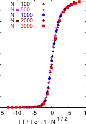
Figure 1: Plot of the data-collapse of the Binder Cumulant versus scaled temperature for various $N$

Data were taken at $T=2.85$ (close to the estimated critical temperature)and $\chi$, $C$ and the Binder cumulant $U_{m}=[{<m^{4}>}/{<m^{2}>}^{2}]_{\rm av}-3$ were calculated, using the single histogram reweighting technique Ferrenberg . We examined lattice sizes $N=100,500,1000,2000,3000$ in our Monte Carlo simulations. We studied $1535$ samples for $N=100$ to $517$ samples for $N=3000$ using $10^{3}$ equilibration and $10^{6}$ MC steps for each $N$. Data were taken at intervals of $10^{3}$ MC steps .

A data-collapse of $U_{m}$ with finite size scaling variable $N^{1/\bar{\nu}}(T-T_{c})/T_{c}$ would give $T_{c}$ (the infinite lattice critical temperature) and $\bar{\nu}$. By using the data-collapse method of Ref. Seno we obtained $T_{c}=2.83(2)$ and $1/\bar{\nu}=0.50(1)$

The value of $\bar{\nu}$ is consistent with previous results Hong . The resulting collapse is shown in Fig. 1. We also investigated similar plots for $\chi$ and $C$ after averaging over many realisations of disorder (not shown here), with same results.

Further proof of the mean-field nature of the transition comes from the comparison of the data with the mean-field form of $U_{m}$. To evaluate the mean field form of $U_{m}$ we use the mean-field form of the magnetisation per spin m probability distribution in the critical region Binder

$$P_{N}(m)\propto\exp{[-N(a_{1}t_{N}m^{2}+a_{2}m^{4})]}$$ (5)

with $t_{N}$ being the critical temperature of a lattice of size $N$ and $a_{1}$, $a_{2}$ being constants. By replacing $\hat{m}=(a_{2}N)^{1/4}m$, we find $U_{m}$ where the averages are obtained by integrating $\hat{m}$ from $-\infty$ to $+\infty$ with the weight

$$P_{N}(\hat{m})\propto\exp{[-b_{1}(x-b_{2})\hat{m}^{2}-\hat{m}^{4}]}$$ (6)

where $b_{1}=a_{1}/{a_{2}}^{1/2}$ , $x$ is the finite size scaling variable $[(T-T_{c})/T_{c}]N^{1/{\bar{\nu}}}$ with $b_{1}b_{2}$ taking care of the finite size shift of the critical temperature. The solid curve in Fig. 1 is obtained with $b_{1}=1.7$, $b_{2}=0.72$.

We find good data collapse by using $\tilde{t}=T-T_{c}$ even though finite size scaling is supposedly better with the use of $\tilde{t}=T-T_{c}(N)$ after finding out the $T_{c}(N)$ for every sample sizeBernardet . This is because our system, as we show, is self-averaging and this method should be more pertinent for non- or weakly self-averaging systems.

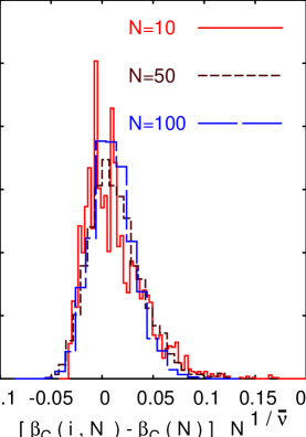
Figure 2: Plot of the distribution of pseudocritical inverse temperatures $\beta_{C}(i,N)$ for various $N$

To investigate the distribution of pseudo-critical temperature, $\beta_{c}(i,N)$ (the temperature at which the specific heat of sample $i$ of size $N$ is a maximum), data were taken at $T=2.85$ and $\beta_{c}(i,N)$ for various $N$ were calculated using the histogram method Ferrenberg . The distribution of $\beta_{c}(i,N)$ for $N=10,50,100$ is constructed.We studied $329$1 lattice samples for $N=10$, $1645$ lattice samples for $N=50$ and $1535$ lattice samples for $N=100$. We find that the inverse critical temperature $\beta_{c}(i,N)$, scales as

$$[(\beta_{c}(i,N)-\beta_{c}(N))^{2}]_{\rm av}\sim N^{-2/{\bar{\nu}}},$$ (7)

which is consistent with Eq. (3), but one also needs a scale factor $N^{-1/2}$ for the probability distribution $P(\beta_{c}(i,N))$. Fig. 2 shows the data collapse of this distribution. The data-collapse is best achieved with $\bar{\nu}=2.00(3)$ which is consistent with the value of $\bar{\nu}$ obtained in the data collapse shown in fig. 1.

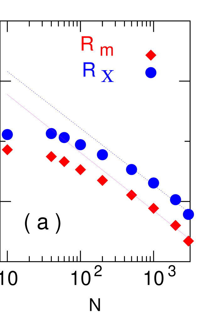
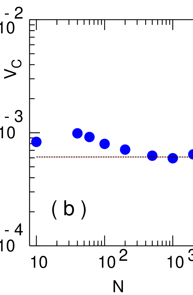
Figure 3: (a) $R_{m}$, $R_{\chi}$ versus $N$ at $T_{C}$ and (b) $V_{C}$ versus $N$ at $T_{C}$.The straight lines show straight line fits to $R_{m}$ and $R_{\chi}$ .

We then studied $R_{m}$, $R_{\chi}$ and $V_{C}$ at $T_{c}^{\infty}$ for the above lattice sizes. About 56440 lattice samples for N=10 to 1000 lattice samples for N=3000 were studied. For each sample we used $10^{3}$ equilibration and $10^{5}$ MC steps. Data were taken at intervals of $10^{3}$ MC steps. The data is fitted to the form $R_{X}=A_{X}\it N^{\rho_{X}}$ where $R_{X}$ is the relative variance for $m$ and $\chi$. The values obtained are $\rho_{m}=-0.96(9)$, and $\rho_{\chi}=-0.94(8)$. Thus $\chi$ and $m$ are strongly self-averaging . The singular part of energy cannot be filtered out and hence the behaviour of $V_{E}$ can not be predicted decisively. We see in Fig. 3 that $V_{C}$ is a constant as expected and hence C is also strongly self-averaging .

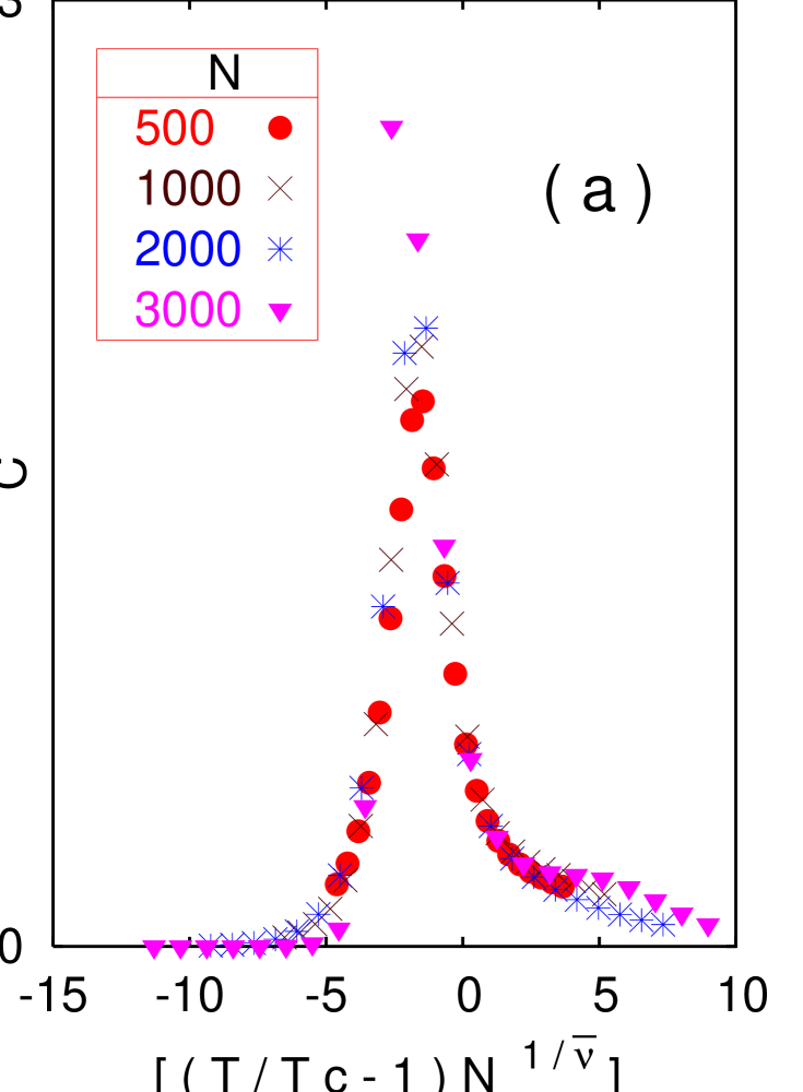
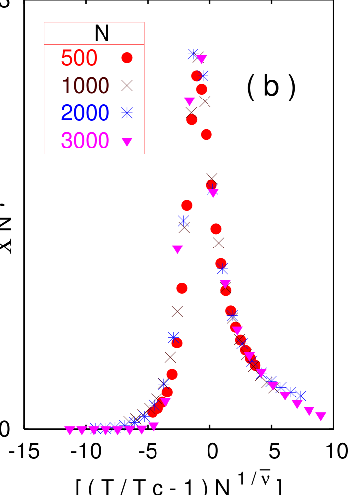
Figure 4: Data collapse of $C$ and $\chi$ on considering a single realisation of randomness

V Discussion

The fact that the peak scales inversely as the width shows that despite the fluctuation in pseudo-critical temperatures,the distribution approaches a $\delta-$function. As a result the critical temperature of a large $N$ network can be thought of as the average of pseudo-critical temperatures of the small sub-networks.This averaging out is tantamount to self-averaging .This is in marked contrast to the other cases of random systems studied so far WD-PRE-98 ; Dillmann ; Marques1 ; Marques2 . It is tempting to conclude that in addition to relevant randomness, a broad distribution of pseudo-critical temperature is a requirement for non-self-averaging.

Whilst in the present work we have used a “canonical” ensemble with a fixed number of bonds, small scale simulations of the Ising model on a SWN in a “grand canonical” ensemble, where the number of bonds can vary, also indicated self-averaging as found here.

In case of a strongly self-averaging system, a typical sample should be a representative of the average. We observe good data collapse with even a single realisation of disorder (as shown in Fig. 4). Thus, in the light of the present work, in such situations, an annealed averaging as done in ref Gitterman should work well. Consequently no extra order parameter like approach should be needed for networks .

It is not clear if this feature of strong self-averaging is a consequence of $\alpha=0$, in which case it could be true for all relevant disorder problems with mean-field behaviour. An extension of the RG argumentAH-PRL-96 to encompass situations with sharp limit of $T_{c}$ distribution and long range interactions, may shed light on this. Whether this result on the disorder aspect of a network is important in other real life situations like the railway network Sen needs further study.

To conclude, we investigated the self-averaging behaviour of the Ising model on a small world network. The distribution of $\beta_{c}(i,N)$ is found to become sharper as $N\to\infty$ with the fluctuation decaying as $[(\delta\beta_{c}(i,N))^{2}]_{\rm av}\sim N^{-2/\bar{\nu}}$. The data collapse of various physical quantities both for a single realisation of disorder and after averaging over many disorder realisations showed no significant difference. At $T_{c}^{\infty}$, the relative fluctuations $R_{m}$, $R_{\chi}$ for magnetization and susceptibility are found to behave as $R_{m},R_{\chi}\sim N^{-1}$ while the variance $V_{C}$ for the specific heat approaches a constant for large $N$. Hence the system is strongly self-averaging in the critical region in spite of relevant randomness. Our results have the following implications. From the small-world networks perspective, the random or statistical features of the network do not play a role in the long range behaviour at the critical point so that one may replace the ensemble of small-world networks by a single average network.

References

- (1) Aharony A. and Harris A. B., Phys. Rev. Lett., 77 (1996) 3700.
- (2) Wiseman S. and Domany E., Phys. Rev. E, 52 (1995) 3469; Phys. Rev. E, 58, (1998) 2938.
- (3) Dillmann O., Janke W. and Binder K., J. Stat. Phys., 92 (1998) 57.
- (4) Marques M.I. and Gonzalo J.A., Phys. Rev. E, 62 (2000) 191.
- (5) Marques M.I. and Gonzalo J.A., Phys. Rev. E, 65 (2003) 057104.
- (6) Watts D. and Strogatz S.H. , Nature 393 (1998) 440.
- (7) Albert R. and Barabasi A.L. , Revs. Mod. Phys., 74 (2002) 47.
- (8) Almaas E., Kulkarni R. V., Stroud D. , Phys. Rev. Lett., 88 (2002) 098101.
- (9) Barrat A. and Weigt M., Eur. Phys. J. B, 13 (2000) 547.
- (10) Gitterman M., J. Phys. A, 33 (2000) 8373.
- (11) Hastings M.B., Phys. Rev. Lett., 91(2003) 098701.
- (12) Herrero C.P., Phys. Rev. E, 65 (2002) 066110.
- (13) Hong H., Kim B.J., Choi M.Y., Phys. Rev. E, 66 (2002) 018101.
- (14) Nikoletopoulos T. et al, J. Phys. A, 37 (2004) 6455.
- (15) Weinrib A. and Halperin B. I., Phys. Rev. B, 27 (1983) 413.
- (16) Lopes J.Viana et al, Phys. Rev. E, 70 (2004) 026112.
- (17) Falcioni M. et al, Phys. Lett. B, 108 (1982) 331 ; Ferrenberg A.M. and Swensden R.H., Phys. Rev. Lett., 61 (1988) 2635.
- (18) Bhattacharjee S.M. and Seno F., J. Phys. A, 34 (2001) 6375.
- (19) Binder K. et al, Phys. Rev. B, 31 (1985) 1498.
- (20) Bernardet K., Pazmandi F. and Batrouni G.G., Phys. Rev. Lett., 84 (2000) 4477.
- (21) Sen P. et al, Phys. Rev. E, 67 (2003) 036106.