Exact theory of kinkable elastic polymers

Abstract

The importance of nonlinearities in material constitutive relations has long been appreciated in the continuum mechanics of macroscopic rods. Although the moment (torque) response to bending is almost universally linear for small deflection angles, many rod systems exhibit a high-curvature softening. The signature behavior of these rod systems is a kinking transition in which the bending is localized. Recent DNA cyclization experiments by Cloutier and Widom have offered evidence that the linear-elastic bending theory fails to describe the high-curvature mechanics of DNA. Motivated by this recent experimental work, we develop a simple and exact theory of the statistical mechanics of linear-elastic polymer chains that can undergo a kinking transition. We characterize the kinking behavior with a single parameter and show that the resulting theory reproduces both the low-curvature linear-elastic behavior which is already well described by the Wormlike Chain model, as well as the high-curvature softening observed in recent cyclization experiments.

I Introduction

The behavior of many semiflexible polymers is captured by the Wormlike Chain modelKratky and Porod (1949); Shimada and Yamakawa (1984). This model amounts to the statistical mechanics of linearly-elastic rodsYamakawa (1997) where the elastic energy is microscopically a combination of both energetic and entropic contributionsNelson (2004). The mechanics of DNA, a polymer of particular biological interest, has been studied extensively experimentally and theoretically and its mechanical properties have been very well approximated by the Wormlike Chain model (WLC)Bustamante et al. (2000) and its successors such as the Helical Wormlike Chain modelShimada and Yamakawa (1984). For example, accurate force-extension experiments have shown that DNA is surprisingly well described by WLCBustamante et al. (2000); Bouchiat et al. (1999); Nelson (2004), at least until the effects of DNA stretching become important at tensions of order 50 pN.

Despite the success of the WLC in describing DNA mechanics, recent DNA cyclization experiments by Cloutier and WidomCloutier and Widom (2004) have shown a dramatic departure from theoretical predictions for highly-curved DNA. These experiments suggest that the effective bending energy of small, cyclized sequences of DNA is significantly smaller than predicted by existing theoretical models based upon linear-elastic constitutive relations, in which the bending energy is quadratic in curvature. Similar anomalies have been revealed in transcriptional regulation where DNA looping by regulatory proteins remains active down to $60$ basepair (bp) separations between the binding sitesBellomy et al. (1988); Rippe et al. (1995); Muller et al. (1996, 1998); Rippe (2001); Zhang et al. (2004).

From a continuum-mechanics perspective, this failure of the model at high-curvature is hardly surprising; the importance of material nonlinearities has been appreciated for many years. In fact, anyone who has ever tried to bend a drinking straw has observed that the straw will at first distribute the bending, as predicted by the linear theory, but as the curvature increases, the straw will eventually kink, localizing the bending. This kinking behavior is the signature of nonlinear constitutive softening at high curvature. Nonlinearities are certainly important in microscopic physical systems, such as polymers, because the effective bending free energy, a combination of interaction potentials and entropic effects, is only approximately harmonic. The possibility of kinking in DNA was realized long ago by Crick and Klug, who proposed a specific atomistic structure for the kink state Crick and Klug (1975). Many authors have since found kinked states of DNA in protein–DNA complexes (see for example Dickerson (1998)), but less attention has been given to spontaneous kinking of free DNA in solution, even though Crick and Klug pointed out this possibility.

Our goal in this paper is to develop a simple, generic extension of the WLC model, introducing only one additional parameter: the average number of kinks per unit length for the unconstrained chain. The “kinks” are taken to be freely-bending hinge elements in the chain. This model is an extension of the well known Wormlike Chain (WLC); we refer to it as the Kinkable Wormlike Chain (KWLC). Although our model is not a detailed microscopic picture for DNA, it does capture the key consequences of any more detailed picture of kink formation. As such, it serves as a useful coarse-grained model to describe high-curvature phenomena in many stiff biopolymers, not just DNA Muroga (1988). Our main results are summarized in figs 5, 6, 10, and 11.

The KWLC is the simplest example of a class of theories that have been proposed and studied by Storm and NelsonStorm and Nelson (2003a) and more recently by LevineLevine (2004). It is simple enough that many results are exact or nearly so. The method by which we obtain our exact results is analogous to the Dyson expansion for time-dependent quantum perturbation theory. For the KWLC, the perturbation series can be re-summed exactly.

For small values of our kinking parameter the KWLC model predicts nearly identical behavior to the WLC—except when the rod is constrained to be highly curved. Such constraints induce kinking, even when the kinking parameter is small. We will show in detail how the energy relief caused by this alternative bending conformation can account for the observed anomalously high cyclization rate of short loops of DNACloutier and Widom (2004) and anomalously high levels of gene expressionMuller et al. (1996, 1998). Further discussion of the applications of KWLC to DNA, will appear elsewhereWiggins et al. (2004); the present paper focuses on the mathematical details of the theory. Yan and Marko, and Vologodskii, have independently obtained results related to ours Vologodskii (2004); Yan and Marko (2004). Also, Sucato et al. have performed Monte Carlo simulations of kinkable chains to obtain information about their structural and thermodynamic properties Sucato et al. (2004).

The outline of the paper is as follows: in section II, we introduce the KWLC model in a discrete form. In section III, we compute the unconstrained partition function for the theory and show that there is a sensible continuum limit. In section IV, we give an exact computation of the tangent partition function of the continuum theory as well the moment-bend constitutive relation and the kink number for bent polymer chains. We show that kinking causes an exact renormalization of the tangent persistence length and we write exact expressions for the average squared end distance and the radius of gyration. In section V, we exactly compute the Fourier-Laplace transform of the spatial propagator and discuss various limits of these results. We also compute the exact force-extension relation and the structure factor for KWLC. In section VI, we compute the KWLC correction to the Jacobson-Stockmayer $J$ factor and the partition function for cyclized chains. We show that the topological constraint of cyclization induces kinking and we compute the kink number distribution explicitly. In section VII, we discuss the limitations of KWLC. In the appendix, we present a summary of the Faltung Theorem which is required for computations and develop the small and large contour length limits of the KWLC $J$ factor.

II Kinkable Wormlike Chain Model

Although the Wormlike Chain model was originally proposed to describe a purely entropic chain without a bending energyKratky and Porod (1949), it is often interpreted as the statistical mechanics of rods with bending energies quadratic in curvatureYamakawa (1997); Landau and Lifshitz (1986). From a mechanical perspective, the success of the WLC model is not surprising since the small amplitude bending of rods universally induces a linear moment response. For WLC, the bending energy for a polymer in configuration $\Gamma$ is

$$E_{\Gamma}=\int_{0}^{L}ds\frac{\xi}{2}\left(\frac{d\vec{t}}{ds}\,\right)^{2}$$ (1)

where $\vec{t}(s)$ is the unit tangent at arc length $s$, $L$ is the contour length, and $\xi$ is the bending modulus. Throughout this paper we will express energies in units of the room-temperature thermal energy $k_{\rm B}T=4.1\times 10^{-21}\,$J. For WLC it is well known that the bending modulus and persistence length (the length scale over which tangent are thermally correlated) are equal in these units Nelson (2004).

It is most intuitive to define our new model in terms of the discretized definition of WLC. Accordingly, we divide a chain of arc length $L$ into $L/\ell$ segments of length $\ell$. There are then $N=(L/\ell)-1$ interior vertices, plus two endpoints (fig 1a). Next we replace the arc length derivative with the finite difference over the segment length $\ell$, replace the integral with a sum, and introduce the spring constant $\kappa\equiv\xi/\ell$. The resulting energy is

$$E_{\Gamma}=\sum_{i=1}^{N}\kappa\left(1-\vec{t}_{i}\cdot\vec{t}_{i-1}\right),$$ (2)

where $\vec{t}_{i}$ is the vector joining vertices $i$ and $i+1$.

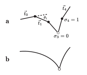
Figure 1: a: The discretized KWLC is a chain of wormlike and kink-like vertices. In this illustration $N=4$; thus there are four vertices, of which one is kink-like. When a vertex $i$ is wormlike ($\sigma_{i}=1$), the energy is given by the normal wormlike chain energy; if it is kink like ($\sigma_{i}=0$), the energy is $\epsilon$, independent of $\theta_{i}$. b: The continuum version of this theory. Although the number of vertices is now infinite, the continuum limit maintains a finite average kink density.

We introduce a similar discretized energy for the Kinkable Wormlike Chain model (KWLC). In addition to the bending angle, there is now a degree of freedom at each vertex describing whether the vertex is kink-like or wormlike. To describe this degree of freedom, we introduce a state variable, $\sigma_{i}$ at each vertex. When $\sigma_{i}=1$, we say that the vertex is wormlike and the energy is given by the discrete WLC energy at that vertex. When $\sigma_{i}=0$, the vertex is kink like and the energy is independent of the bend angle at that vertex, but there is an energy penalty $\epsilon$ to realize the kink state. This model is depicted schematically in fig 1. The energy for the model we have just described can be concisely written as

$$E^{*}_{\Gamma}=\sum_{i=1}^{N}\left[\kappa\left(1-\vec{t}_{i}\cdot\vec{t}_{i-1}\right)\sigma_{i}+\epsilon(1-\sigma_{i})\right]\ ,$$ (3)

where the $*$ denotes that this is the energy of the KWLC theory and $\epsilon$ is the energetic cost of introducing a kink in the chain. Note that in general we denote KWLC results or equations with a $*$. We will recover the WLC results when we take the kinking energy $\epsilon$ to infinity. While Storm and NelsonStorm and Nelson (2003b) and othersMarko (1998); Ahsan et al. (1998); Cizeau and Viovy (1997); Rouzina and Bloomfield (2001); Storm and Nelson (2003b); Levine (2004) have considered more general theories where the kink energy is not assumed to be independent of the kink angle, much of the important physics can already be studied in the simpler KWLC theory. Moreover, this theory has the significant advantage of being analytically exact to a much greater extent than more general theories; it applies in the limit where the kinks are only weakly elastic compared to the elastic rod.

III Partition functions

For a summary of notation used in this article, see Appendix D.

We have defined the KWLC model in terms of a discrete set of degrees of freedom. In the next section, however, we shall wish to take advantage of the continuum WLC machinery. To this end, this section formulates the continuum limit of the KWLC model. Beyond the computational advantage, there is also an additional reason to go to the continuum limit. Fig 1 describes the kinking with two parameters, a density $\ell^{\raise 0.45206pt\hbox{${\scriptscriptstyle-}$}\kern-0.35002pt1}$ of kinkable sites and the kink energy $\epsilon$. We wish to describe the kinking in terms of a single parameter, to be called $\zeta$ (see eqn 7). $\zeta$ essentially sets the average number of kinks per contour length for a long, unstressed chain. In the continuum limit of WLC, we take $\ell\to 0$ while holding the persistence length $\xi$ and chain length $L$ constant. To take the corresponding continuum limit for KWLC, we will also hold $\zeta$ constant as $\ell\to 0$.

We begin by computing the partition functions for the WLC and KWLC and demonstrating that there is a continuum limit of the KWLC. These unconstrained partition functions are required for later computations. For this case, the partition function factors into independent contributions from each interior vertex. In the continuum limit ($\kappa\rightarrow\infty$), the partition function for each vertex in the WLC model is

$$Q\equiv\lim_{\kappa\rightarrow\infty}\int d^{2}\vec{t}_{i}\ \exp\left[-\kappa(1-\cos\theta_{i})\right]=\frac{2\pi}{\kappa},$$ (4)

where $\theta_{i}$ is the polar angle of $\vec{t}_{i}$ defined using $\vec{t}_{i-1}$ as the polar axis, that is, $\cos\theta_{i}\equiv\vec{t}_{i}\cdot\vec{t}_{i-1}$. The measure $d^{2}\vec{t}_{i}=d(\cos\theta_{i})d\phi_{i}$ denotes solid angle on the unit sphere. The total discretized partition function for the chain of $N+1$ segments is then

$${\cal Z}_{\mathrm{discrete}}(L)=4\pi Q^{N}.$$ (5)

The factor of $4\pi$ reflects one overall orientation integral, for example the integral over $\vec{t}_{0}$.

Similarly, the partition function for a single vertex of the KWLC theory is

$$Q^{*}\equiv\lim_{\kappa\rightarrow\infty}\int d^{2}\vec{t}_{i}\ \left(\exp\left[-\kappa(1-\cos\theta_{i})\right]+\exp\left[-\epsilon\right]\right)=Q\left(1+2\kappa e^{-\epsilon}\right),$$ (6)

which we have written in terms of the corresponding WLC quantity $Q$. The total partition function for the chain of $N+1$ segments is ${\cal Z}^{*}_{\mathrm{discrete}}(L)=4\pi(Q^{*})^{N}$.

In the small segment length limit, eqn 6 shows that the probability of a vertex being kink-like is $2\kappa e^{-\epsilon}$. Therefore the probability of kinking per unit length (for this unconstrained situation) is

$$\zeta\equiv\frac{2\xi}{\ell^{2}}e^{-\epsilon}=\frac{4\pi}{\ell Q}e^{-\epsilon},$$ (7)

where we have eliminated the bending spring constant, $\kappa$, in favor of the persistence length, $\xi=\kappa\ell$. In order to recover a sensible continuum limit, we will hold the parameter $\zeta$ constant as we take the segment length to zero. Note that we recover the WLC theory when we set $\zeta\to 0$. In later sections we will discuss a formal “zero temperature” limit, in which simple mechanics (no thermal fluctuations) describes the physics. This limit is a useful intuitive tool, not an experimental prediction of the behavior of polymers frozen in solution. The “zero temperature” limit is taken treating $\zeta$ as temperature independent, which is equivalent to either the short rod limit or the large persistence length limit which we shall use interchangeably.

In the continuum limit, we must remove a divergent constant in the partition functions as $N\to\infty$. Thus we define the path integral measure

$$[d\vec{t}\,(s)]_{\vec{t}_{\rm i}}\,\equiv\prod_{i=1}^{N}\frac{d^{2}\vec{t}_{i}}{Q},$$ (8)

where $Q$ is defined by eqn 4. Note that unlike the discrete case, in this measure the starting tangent vector $\vec{t}_{0}$ is not integrated, but is instead fixed to some given $\vec{t}_{\rm i}$. The continuum partition function corresponding to ${\cal Z}_{\mathrm{discrete}}(L)$ is then

$${\cal Z}(L)\equiv\int[d\vec{t}\,(s)]_{\vec{t}_{\rm i}}\,e^{-E^{*}}=1.$$ (9)

With our choice of integration measure, ${\cal Z}(L)$ just equals one, independent of $L$.

The continuum KWLC partition function is now

$${{\cal Z}^{*}}(L)=\lim_{N\rightarrow\infty}\left(1+\frac{\zeta L}{N}\right)^{N}=e^{\zeta L}.$$ (10)

The convergence of the partition function assures us that the continuum limit is well defined. As a consistency check, we now compute the average kink number for the unconstrained chain

$$\left<m\right>=\frac{\partial\log{\cal Z}^{*}}{\partial\log\zeta}=\zeta L,$$ (11)

which confirms that $\zeta$ is indeed density of kinks. The expansion of the partition function in a power series shows that the kink number distribution is also correct. We will repeat the average kink number calculation several times in the course of this paper for different constraints to show that constraining the chain will affect the kink number.

IV Tangent partition function and propagator

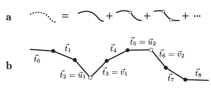
Figure 2: a. Diagrammatic representation of the kink expansion for the tangent partition function. The dashed curve represents the KWLC theory and the solid curves represent the WLC theory. It is convenient to collect the terms by kink number as shown. b.  Detail of the two-kink term, showing the relation to the underlying discrete model. $\vec{u}_{i}$ and $\vec{v}_{i}$ are the tangent vectors flanking kink number $i$.

In this section we compute the tangent partition function and propagator by using a method symbolized in fig 2a. By tangent partition function ${\cal Z}(\vec{t}_{\rm f},\vec{t}_{\rm i},L)$ we mean the partition function with the initial and final tangents constrained (eqn 12 below). Dividing the tangent partition function by the unconstrained partition function ${\cal Z}(L)$ gives the probability density $H(\vec{t}_{\rm f},\vec{t}_{\rm i},L)$ for the final tangent vector, given the initial tangent. We will refer to $H$ as the normalized tangent partition function, or propagator.

Most of the kink-related physics of the KWLC theory can be understood qualitatively from the tangent partition function. Furthermore, the computation of the tangent partition function is more transparent than the analogous spatial computation in which the end-to-end distance is constrained along with the initial and final tangents. The tangent partition function for WLC is defined as

$${\cal Z}(\vec{t}_{\rm f},\vec{t}_{\rm i};L)\equiv\int[d\vec{t}\,(s)]_{\vec{t}_{\rm i}}\,\ e^{-E}\ \delta^{(2)}[\,\vec{t}_{N}-\vec{t}_{\rm f}\ ],$$ (12)

where the path integral is regularized as described above (eqn 8). Due to the tangent constraint, the partition function no longer factors into independent vertex contributions. The lower limit on the integration denotes that the initial tangent $\vec{t}_{0}$ is held equal to $\vec{t}_{\rm i}$; the final tangent $\vec{t}_{N}$, is set to $\vec{t}_{\rm f}$ by the delta function. We integrate (or sum) over the infinite set of intervening tangents in order to generate the partition function. In this regularization scheme, the tangent partition function and tangent propagator are identical

$$H(\vec{t}_{\rm f},\vec{t}_{\rm i};L)={\cal Z}(\vec{t}_{\rm f},\vec{t}_{\rm i};L),$$ (13)

since with our conventions the unconstrained WLC partition function is one. However, we will see that this convenient identity does not hold for the KWLC: $H^{*}\not={\cal Z}^{*}$.

While the direct evaluation of the path integral in eqn 12 is difficult, it is well known that this calculation is equivalent to finding the quantum-mechanical propagator for a particle on the unit sphereFeynman and Hibbs (1965); Grosberg and Khokhlov (1994). The tangents correspond to position, arc length corresponds to imaginary time, and persistence length corresponds to mass. Thus, the tangent partition function is

$${\cal Z}(\vec{t}_{\rm f},\vec{t}_{\rm i};L)=\left<\vec{t}_{\rm f}\,\right|e^{-{\cal H}L}\left|\vec{t}_{\rm i}\right>,$$ (14)

where the Hamiltonian operator is defined as

$${\cal H}\equiv\frac{\vec{p}^{\ 2}}{2\xi},$$ (15)

where $\vec{p}^{\ 2}$ is the Laplace operator on the unit sphere. The Hamiltonian is diagonal in the angular momentum representation so the tangent partition function for WLC can be expressed as

$${\cal Z}(\vec{t}_{\rm f},\vec{t}_{\rm i};L)=\sum^{\infty}_{l=0}\sum_{m=-l}^{l}Y^{m}_{l}(\vec{t}_{\rm f}{\,})Y_{l}^{m}(\vec{t}_{\rm i})^{*}C_{l}(L).$$ (16)

In this expression, the $Y_{l}^{m}$’s are the Spherical Harmonics and the coefficients $C_{l}$ are

$$C_{l}(L)=\exp\left[-\frac{l(l+1)L}{2\xi}\right].$$ (17)

It can easily be shown that this partition function has the required normalization by summing over the final tangent to recover ${\cal Z}(L)=1$.

To compute the tangent partition function for KWLC, we proceed with the path integral in exactly the same fashion, setting the initial tangent, integrating over an infinite set of intervening tangents, and summing over the state vectors:

$${\cal Z}^{*}(\vec{t}_{\rm f},\vec{t}_{\rm i};L)=\sum_{\{\sigma_{1},\ldots,\sigma_{N}\}}\int[d\vec{t}\,(s)]_{\vec{t}_{\rm i}}\,\ e^{-E^{*}}\ \delta^{(2)}[\,\vec{t}_{N}-\vec{t}_{\rm f}\ ].$$ (18)

It is now convenient to collect the terms in contributions with a fixed number $m$ of kinks and then express the result in the continuum limit.

The first step in going from the definition of the discrete KWLC tangent partition function to the continuum limit is to reorganize the sum over $\{\sigma_{n}\}$ as a sum over the number of kinks $m$. Each term of this sum is in turn a sum over the positions $n_{i}$ of the kinks, for $i=1,\ldots m$. The only subtlety here is introducing the correct limits on the sum to avoid over counting the kink states. The last kink can be chosen at any arc-length location, but additional kinks must always be chosen with smaller arc-length values than the following kink. This method is more convenient than introducing “time ordering” and a factor of $1/m!$ to explicitly remove the over counting as is commonly done in the Dyson expansion for time-dependent quantum perturbation theorySakurai (1994).

The next step is to replace the kink position sums with integrals over the position of the kinks as

$$\sum_{n_{i}=i}^{n_{i+1}-1}\rightarrow\int_{0}^{L_{i+1}}\frac{dL_{i}}{\ell},\qquad i=1,\ldots m\ ,$$ (19)

where $L_{i}\equiv n_{i}\ell$ and we take $L_{m+1}=L$. The structure of the arc length integrals is that of a series of convolutionsArfken and Weber (1995), which we write symbolically as $\otimes$. For example, if $F(L)$ and $G(L)$ are two functions, then

$$(F\otimes G)(L)\equiv\int_{0}^{L}\,dL_{1}\ F(L-L_{1})G(L_{1})\ .$$ (20)

In the intervals between kinks, the chain is described by the WLC energy function. We can therefore replace each partial path integral with a WLC propagator.

For every kink, there is one factor of $Q^{\raise 0.45206pt\hbox{${\scriptscriptstyle-}$}\kern-0.35002pt1}$ that has been introduced by the path integral normalization (eqn 8) but is not absorbed by the definition of the WLC propagator (eqns 18 and 13). The $m$ factors of $\ell^{\raise 0.45206pt\hbox{${\scriptscriptstyle-}$}\kern-0.35002pt1}$, $e^{-\epsilon}$, and $Q^{\raise 0.45206pt\hbox{${\scriptscriptstyle-}$}\kern-0.35002pt1}$ can now be written as $(\zeta/4\pi)^{m}$ (see eqn 7). Defining ${\cal Z}^{*}=\sum_{m}{\cal Z}^{*}_{m}$, the terms in the kink-number expansion can thus be written (compare fig 2)

$${\cal Z}^{*}_{m}(\vec{t}_{\rm f},\vec{t}_{\rm i};L)=\zeta^{m}\int\prod_{j=1}^{m}\frac{d^{2}\vec{u}_{j}d^{2}\vec{v}_{j}}{4\pi}\ \underbrace{\left(H(\vec{t}_{\rm f},\vec{v}_{m})\otimes H(\vec{u}_{m},\vec{v}_{m-1})\otimes\cdots\otimes H(\vec{u}_{1},\vec{t}_{\rm i})\right)}_{m+1}(L),$$ (21)

The $2m$ angular integrations are over the incoming ($\vec{u}_{i}$) and outgoing ($\vec{v}_{i}$) tangents of the $m$ kinks.

Eqn 21 has a very simple interpretation. The probability of creating a kink between $L$ and $L+dL$ is just $\zeta dL$. We then sum over all possible configurations being careful to choose the integration limits so as not to over count the kink states. At each kink, all orientational information is lost, so that only tangent independent terms of the propagator contribute (those with angular quantum number $l=0$).

To compute the contour length convolution of propagators, it is convenient to work with the contour length Laplace transformed propagators $\tilde{H}$ (eqn 80). We shall denote the contour length Laplace transformed functions with a tilde and use the variable $p$ as the arc length Laplace conjugate variable. Although we could avoid Laplace transforming the partition function at this juncture, we use this method presently because it is analogous to our later computation of the spatial propagator. By the well known Faltung theorem (eqn 84), the convolution of propagators is just the product of Laplace transforms. Therefore, in terms of the transformed WLC propagators, the $m$ kink KWLC Laplace transformed partition function is

$$\tilde{\cal Z}^{*}_{m}(\vec{t}_{\rm f},\vec{t}_{\rm i};p)=\zeta^{m}\begin{cases}\tilde{H}(\vec{t}_{\rm f},\vec{t}_{\rm i};p),&m=0\\ \tilde{C}_{0}^{m+1}(p)/4\pi,&m>0\ .\\ \end{cases}$$ (22)

To derive eqn 22, note that eqn 16 gives the WLC tangent propagator summed over the initial tangent as $C_{0}(L)$, which equals 1 from eqn 17. The corresponding Laplace transform is just $\tilde{C}_{0}(p)=1/p$.

The $m$ kink contributions to the KWLC transformed tangent partition function can now be summed exactly (i.e. ${\cal Z}^{*}=\sum_{m}{\cal Z}^{*}_{m}$) because they form a geometric series, resulting in

$$\tilde{\cal Z}^{*}(\vec{t}_{\rm f},\vec{t}_{\rm i};p)=\tilde{H}(\vec{t}_{\rm f},\vec{t}_{\rm i};p)+\frac{1}{4\pi}\frac{\zeta\tilde{C}_{0}^{2}(p)}{1-\zeta\tilde{C}_{0}(p)}\ .$$ (23)

The $m>0$ kink terms clearly contribute no tangent dependence. The inverse Laplace transform can now be computed without complications, giving the exact KWLC tangent partition function

$${\cal Z}^{*}(\vec{t}_{\rm f},\vec{t}_{\rm i};L)=H(\vec{t}_{\rm f},\vec{t}_{\rm i};L)+\frac{e^{\zeta L}-1}{4\pi}.$$ (24)

Alternatively, we could have derived eqn 24 by noting that the KWLC model is mathematically equivalent to a Quantum Mechanical system whose Hamiltonian is diagonal in the angular momentum representation:

$${\cal H}^{*}=-\zeta\ \left|0,0\right>\otimes\left<0,0\right|+{\cal H}\ .$$ (25)

Here $\left|\,l,m\right>$ is the state with angular momentum quantum numbers $l$ and $m$ and $\cal H$ is the Hamiltonian operator for the WLC. The only change to the theory is a “ground state energy” shift equal to $-\zeta$.

The KWLC tangent propagator and its Laplace transform can now be evaluated using eqn 10:

$$H^{*}(\vec{t}_{\rm f},\vec{t}_{\rm i};L) = \frac{{\cal Z}^{*}(\vec{t}_{\rm f},\vec{t}_{\rm i};L)}{{\cal Z}^{*}(L)}=e^{-\zeta L}\left[H(\vec{t}_{\rm f},\vec{t}_{\rm i};L)+\frac{e^{\zeta L}-1}{4\pi}\right],$$ (26)

$$\tilde{H}^{*}(\vec{t}_{\rm f},\vec{t}_{\rm i};p) = \tilde{H}(\vec{t}_{\rm f},\vec{t}_{\rm i};p+\zeta)+\frac{\zeta}{4\pi p(p+\zeta)}.$$ (27)

Fig 3a compares the KWLC tangent propagator to the WLC theory with an illustrative value $\zeta=0.01/\xi$. The two theories appear indistinguishable, and in fact we will find that many, but not all, predictions of the models are essentially the same in this parameter regime.

In principle since the propagator is known exactly, everything in the theory can now be computed. Of course this is an exaggeration since, even though the tangent propagator for WLC has long been known, only recently have the exact expressions for the transformed spatial propagator been derivedSpakowitz and Wang (2004); Stepanow and Schutz (2002). The free energy of the chains for both theories have the canonical relation with their respective partition functions:

$$F(\theta;L)=-\log{\cal Z}(\vec{t}_{\rm f},\vec{t}_{\rm i};L),$$ (28)

where we have explicitly written the free energy in terms of the deflection angle defined by the dot product of the initial and final tangents: $\cos\theta=\vec{t}_{\rm i}\cdot\vec{t}_{\rm f}$. Up to this point we have written the partition function and propagator as explicit functions of both the initial and the final tangent but the rigid body rotational invariance of the energy implies that these functions depend only on the deflection angle. To express any quantity in terms of the deflection angle, we set the initial tangent to be the unit vector in the $z$ direction and the final tangent to be the unit vector in the radial direction. $\theta$ now assumes its canonical definition in spherical polar coordinates.

Fig 3b compares the free energies of WLC and KWLC. Despite the similarity of propagators (fig 3a), the free energies are quite different. To understand the significance of this free energy, we imagine discretizing the chain at some segment length $\ell$. The free energy $F(\theta;\ell)$ gives us the effective constitutive relation for single-state torsional springs in this new discretized theory. As depicted is fig 3b, the potential energy of these springs is initially quadratic in deflection, but saturates due to kink formation.

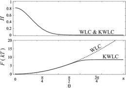
Figure 3: The tangent propagator and the tangent free energy as functions of the deflection angle for the illustrative values $L=0.2\xi$ and $\zeta\xi=10^{-2}$. The solid curves are KWLC and the dashed curves are WLC with the same value of $\xi$. In the absence of kinking, the WLC distribution ($H$) is essentially zero away from small deflection. For the small value of $\zeta$ chosen above, WLC and KWLC are indistinguishable in the top panel. The presence of kinks adds a background level to the propagator which is independent of $\theta$, but is thermally inaccessible—too small to distinguish from zero in the top panel, but is visible in the free energy in the lower panel. The tangent free energy gives an intuitive picture of the system interpreted as as single-state system with an effective bending modulus which saturates due to kinking. Most thermally driven experiments measure the polymer distribution as it is pictured in the top panel and are therefore insensitive to the high-curvature constitutive relation. But experiments which do probe this regime, short-contour-length cyclization for example, will be extremely sensitive to the difference between the theories due to the large free energy difference at large deflection.

IV.1 Moment-Bend & kink number

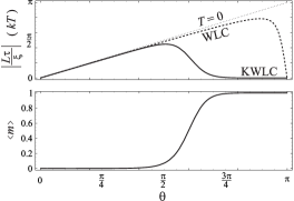
Figure 4: The bending moment $\tau$ and average kink number $\langle m\rangle$ as functions of the tangent deflection angle for illustrative values $L=0.2\xi$ and $\zeta\xi=10^{-2}$. The solid curves are KWLC and the dashed curves are WLC with the same bend persistence length. At small $\theta$, the normalized bending moment exhibits a linear spring dependence and the chain is unkinked. The limiting linear behavior of the short rod limit is the dotted curve, labeled $T=0$ corresponding to the mechanical limit of WLC. For large deflection, the chain kinks and the moment drops to zero. This correspondence between kinking and the moment is clearly illustrated in the short length limit depicted above.

To understand the interplay between chain kinking and deflection, it is helpful to explicitly compute the relation between the deflection angle and the restoring moment (torque), as well as computing the average kink number. Here we ask the reader to imagine a set of experiments analogous to force-extension but where the moment-bend constitutive relation is measured. We compute the constitutive relation in the usual way in terms of the deflection angle $\theta$

$$\tau(\theta;L)\equiv-\frac{\partial}{\partial\theta}F(\theta;L),$$ (29)

where $F(\theta;L)$ is the tangent free energy and $\theta$ is the deflection angle. In terms of the WLC bending moment, eqn 24 shows that the moment for KWLC has a very simple form:

$$\tau^{*}(\theta;L)=\tau(\theta;L)\frac{{\cal Z}(\theta;L)}{{\cal Z}^{*}(\theta;L)},$$ (30)

where $\tau$ is the WLC moment and ${\cal Z}$ and ${\cal Z}^{*}$ are the tangent partition functions for WLC and KWLC, respectively. The moment is plotted as a function of deflection in fig 4. For short chains, the small deflection moments of the two theories initially coincide. But as the deflection increases, there is a transition, corresponding to the onset of kinking, where the moment is dramatically reduced to nearly zero. In eqn 30, this transition is clear from the ratio of the partition functions. Remember that the KWLC partition function is the sum of the WLC partition function and the $m>0$ kink partition functions. Before the onset of kinking, the WLC and KWLC partition functions are equal since the kinked states do not contribute significantly to the partition function. For large deflection, the KWLC partition function is kink dominated and therefore the ratio in eqn 30 tends to zero. Physically, once the chain is kink dominated, the moment must be zero since the kink energy is independent of the kink angle. At zero temperature, the moment would be zero, but fluctuations in which the chain becomes unkinked cause the moment to be nonzero. We discuss this effect in more detail below.

To explicitly see that the reduction in the moment corresponds to kinking, we compute the average kink number as a function of deflection:

$$\left<m\right>(\theta;L)=-\frac{\partial F^{*}}{\partial\log\zeta}=\frac{\zeta L}{4\pi H^{*}(\theta;L)}\ ,$$ (31)

which is depicted in fig 4. Note that when we remove the tangent constraint, we again find that the average kink number is $\zeta L$. When the chain is constrained, the enhancement factor is proportional to $(H^{*})^{\raise 0.45206pt\hbox{${\scriptscriptstyle-}$}\kern-0.35002pt1}$. Note that this implies that the kink number will be reduced when the tangents are constrained to be aligned and enhanced when the chain is significantly bent. In fig 4, the kink-induced reduction in the moment can be seen to correspond to the rise of the kink number from zero to one kink.

We will now compare these exact results to the mechanical or “zero temperature” limit. This regime is equivalent to the large persistence length limit, where we can write the partition function concisely as

$$\lim_{L\rightarrow 0}{\cal Z}^{*}(\vec{t}_{\rm f},\vec{t}_{\rm i};L)=\frac{1}{4\pi}\left[\frac{2\xi}{L}\exp\left(-\frac{\xi}{2L}\theta^{2}\right)+\zeta L\right]\ ;$$ (32)

the WLC limit is recovered for $\zeta=0$. In the short length limit, the moment of the WLC chain is simply linear in deflection: $\tau=-\theta\xi/L$. This moment is also plotted in fig 4. Even without the complication of kinking, there is already one interesting feature of the exact WLC moment-bend constitutive relation which needs explanation. For large deflection, the linear relation already fails in the WLC model! This is a thermal effect which is best understood by going to the extreme example of deflection $\theta=\pi$. For any configuration, the contribution of a chain reflected through the axis defined by the initial tangent will make the partition function symmetric about $\vec{t}_{\rm f}=-\vec{t}_{\rm i}$. This implies that the bending moments from these chains cancel. Away from $\theta=\pi$, the cancellation is no longer exact. In the mechanical limit, this effect is present but localized at $\theta=\pi$ due to the path degeneracy.

In the mechanical limit, kinking is always induced by bending and at most one kink is nucleated. In this limit, the KWLC bend-moment can be rewritten in terms of the kink number

$$\tau^{*}(\theta;L)=\tau(\theta;L)(1-\left<m\right>),$$ (33)

where the kink number is just the Heaviside step function,

$$\left<m\right>(\theta,L)=\Theta_{H}[\theta-\theta_{0}],$$ (34)

around a critical deflection angle

$$\theta_{0}\equiv\left[\frac{2L}{\xi}\log\frac{2\xi}{\zeta L^{2}}\right]^{1/2}.$$ (35)

For deflection less than the critical deflection, the kink number is zero and the moment is given by the WLC moment. At the critical deflection angle, there is an abrupt transition to the kinked state with kink number one and the moment zero. Precisely at the critical angle the free energy of the kinked state and the elastically bent state are equal. Note that we have not discussed dynamics and have assumed that the system is in equilibrium, not kinetically trapped.

The behavior of the KWLC theory for short contour lengths is nearly what one would expect from mechanical intuition. Bending of the chain on short length scales induces a moment which is initially linearly dependent on deflection. When the chain is constrained to a large deflection angle, kinking is induced and the response of the chain to deflection is dramatically weakened. In the mechanical limit, once kinking is induced, the moment is zero but for finite size rods, the ability of the chain to fluctuate between the kinked states and unkinked states blurs the dramatic zero-temperature transition between the kinked and unkinked bend response.

Our discussion here has focused principally on developing an intuition for the short chain limit. From an experimental perspective, it is difficult to measure the moment-bend relation directly as we have described, especially for short chains. While single molecule AFM experiments might probe this relation, most of the information about the moment-bend constitutive relation comes from indirect measurements of thermally-induced bending. For example light scattering, force-extension, and cyclization experiments are all measures of thermally induced bending. As we shall explain, only cyclization experiments with short contour length polymers are sensitive to the high curvature regime of the moment-bend constitutive relation. For the most part, these thermally driven bending experiments are only sensitive to the thermally accessible regime of the moment-bend constitutive relation which corresponds to small curvature and therefore small deflection on short length scales, a regime that is very well approximated by linear moment-bend constitutive relation. For long chains, the initial linear response is weaker implying that the kinking transition is less pronounced. In fact we shall see in the next section that for some of these indirect measurements of the low curvature regime of the constitutive relation, the effect of the kinking will be indistinguishable from the linear elastic response.

IV.2 Persistence length

Since many polymer characterization experiments are most sensitive to the thermally-accessible weak-bending regime, it is clearly of interest to determine whether kinking changes this low-curvature physics. Intuitively, we have already argued that, at least for small kink densities, many properties of the polymer that do not explicitly probe the highly bent structure will remain essentially unchanged. In this section, we will derive a number of exact results that show that the effects of kinking can be described by a renormalization of the persistence length of WLC theory for some bulk features of the polymer distribution, regardless of the magnitude of $\zeta$.

The tangent-tangent correlation must be a decreasing exponential due to multiplicativityNelson (2004); Grosberg and Khokhlov (1994) and therefore we can discuss the decay length. The tangent persistence is

$$\left<\vec{t}_{\Delta}\cdot\vec{t}_{0}\right>=e^{-(\zeta+\xi^{-1})\Delta},$$ (36)

which can be computed by examining the limit of small $\Delta$ and applying the tangent propagator (eqn 26). Since this result is identical to the WLC result except for the decay constant, we introduce the effective persistence length

$$\xi^{*}\equiv\left(\xi^{-1}+\xi_{\rm kink}^{-1}\right)^{-1},$$ (37)

where the kink length is defined as $\xi_{\rm kink}\equiv\zeta^{-1}$. The form of this effective persistence length is not surprising since a roughly analogous effect is observed adding two linear springs together or from the combination of static and dynamic persistence lengthTrifonov et al. (1987); Nelson (1998); Wiggins and Nelson (2004). This tangent persistence result immediately implies that an analogous exact renormalization occurs for both the mean squared end distance

$$\left<R^{2}\right>_{\rm KWLC}=\left[\left<R^{2}\right>_{\rm WLC}\right]_{\xi\rightarrow\xi^{*}}=2L\xi^{*}-2{\xi^{*}}\left(1-e^{-L/\xi^{*}}\right)$$ (38)

and the radius of gyration

$$\left<R^{2}_{g}\right>_{\rm KWLC}=\left[\left<R^{2}_{g}\right>_{\rm WLC}\right]_{\xi\rightarrow\xi^{*}}=\frac{L{\xi^{*}}}{3}-{\xi^{*}}^{2}+\frac{{2\xi^{*}}^{3}}{L}-\frac{2{\xi^{*}}^{4}}{L^{2}}\left(1-e^{-L/{\xi^{*}}}\right),$$ (39)

since these result are simply integrations of the tangent persistenceYamakawa (1997). In experiments sensitive only to the radius of gyration (static scattering for small wave number) or the average square end distance (force-extension in the small force limit), the measured persistence length of the KWLC theory will be the effective persistence length, $\xi^{*}$, regardless of the magnitude of $\zeta$. In most systems of physical interest, the kink length is much larger than the bend persistence length implying that, even if the bend persistence were independently measurable, the difference between the effective persistence length and the bend persistence length would be very small. In other words, the loss of tangent persistence due to kinking is negligible compared with the loss due to thermal bending since kinks are rare on the length scale of a persistence length.

The tangent persistence corresponds to the first moment of the tangent propagator. Clearly the renormalization we have discussed fails for higher order moments! At least in principle it is therefore possible to determine the bend persistence from higher order moments of the distribution. From an experimental perspective this corresponds to scattering experiments at large wave number, force extension for large force, or cyclization experiments for short contour length. To predict the effects of kinking in these experiments, we must compute the spatial propagator (the spatial distribution function).

V Tangent-spatial and spatial propagators

The spatial propagator $K(\vec{x};L)$ is defined as the probability density of end displacement $\vec{x}$ for a polymer of contour length $L$. Similarly, the tangent-spatial propagator $G(\vec{x};\vec{t}_{\rm f},\vec{t}_{\rm i};L)$ is defined as the probability density of end displacement $\vec{x}$ with final tangent $\vec{t}_{\rm f}$, given an initial tangent $\vec{t}_{\rm i}$, for a chain of contour length $L$. Although in principle the theory is solved once the tangent propagator is known, the moments of the spatial propagator, or spatial distribution function, are more experimentally accessible than the tangent propagator. In particular, the $J$ factor measured in cyclization experiments, the force-extension characteristics, and the structure factor measured in scattering experiments are all more directly computable from the propagators $G$ and $K$. In this section, we first compute the spatial propagator and then discuss its application to experimental observables.

Following our computation of the tangent propagator, we compute the tangent-spatial and spatial partition functions. Our solution relies on the same Dyson-like expansion of the partition function in the kink number as was exploited to compute the tangent partition function. The only added complication is that, in addition to the arc length convolution, we must also compute convolutions over the 3d spatial positions of the kinks. By going to the Fourier-Laplace transformed propagator, the convolutions again become products and the $m$ kink contributions can be summed exactly. Unfortunately the exact results of this computation will only be found analytically up to a Fourier-Laplace transform, in part because the WLC theory itself is only known analytically in this formSpakowitz and Wang (2004); Stepanow and Schutz (2002).

We begin by writing the tangent-spatial partition function for the KWLC theory in an form analogous to the tangent partition function in eqn 18:

$${\cal Z}^{*}(\vec{x};\vec{t}_{\rm f},\vec{t}_{\rm i};L) = \sum_{\{\sigma_{1},\ldots,\sigma_{N}\}}\int[d\vec{t}\,(s)]_{\vec{t}_{\rm i}}\,\ e^{-E^{*}}\delta^{(2)}[\,\vec{t}_{N}-\vec{t}_{\rm f}\ ]\delta^{(3)}[\,\vec{x}_{N+1}-\vec{x}\ ],$$ (40)

where $\vec{t}_{0}$ is the initial tangent vector. The additional spatial Dirac delta function in the equation sets a spatial constraint for the end displacement; in this expression, $\vec{x}_{N+1}\equiv\ell\sum_{n=0}^{N}\vec{t}_{n}$. We will again collect the terms in this sum by kink number $m$. In the intervals between kinks, we again introduce the WLC propagator, but this time we use the tangent-spatial propagator $G$, defined by an expression analogous to eqn 40, but with $E$ in place of $E^{*}$.

Because we have normalized the unconstrained WLC partition function such that ${\cal Z}\equiv 1$, the tangent-spatial partition function and propagator are identical. It is convenient to introduce the WLC spatial propagator

$$K(\vec{x};L)\equiv\frac{1}{4\pi}\int\,d^{2}\vec{t}_{1}d^{2}\vec{t}_{2}\ G(\vec{x};\vec{t}_{1},\vec{t}_{2};L),$$ (41)

where we sum over the final tangent and average over the initial tangent to derive the spatial probability density. We also introduce the one tangent summed tangent-spatial propagator

$$G^{\prime}(\vec{x},\vec{t};L)=\int d^{2}\vec{t}_{1}\ G(\vec{x};\vec{t},\vec{t}_{1};L),$$ (42)

which will allow us to concisely express intermediate results. Finally for economy of notation, we write the convolutions over both the spatial position and arc length symbolically with $\otimes$, generalizing the notation introduced in Sect. IV.

The $m>0$ kink KWLC tangent-spatial partition function can be written in terms of the WLC propagators:

$${\cal Z}^{*}_{m}(\vec{x};\vec{t}_{\rm f},\vec{t}_{\rm i};L)=\frac{\zeta^{m}}{4\pi}\left(G^{\prime}(\vec{t}_{\rm f})\otimes\left[K\otimes\,\right]^{m-1}G^{\prime}(\vec{t}_{\rm i})\right)(\vec{x},L)\ ,\quad m>0\ .$$ (43)

We now introduce the WLC Fourier-Laplace transforms of the propagators $G^{\prime}$ and $K$. We denote the transformed functions with a tilde. The Laplace conjugate of contour length $L$ is $p$ and the Fourier conjugate of the end displacement $\vec{x}$ is the wave number $\vec{k}$. The Faltung theorem (Eqs 79 and 84) allows us to replace the spatial-arc length convolutions with the products of the Fourier-Laplace transformed propagators. The $m$ kink KWLC transformed partition function is

$$\tilde{\cal Z}^{*}_{m}(\vec{k};\vec{t}_{\rm f},\vec{t}_{\rm i};p)=\zeta^{m}\begin{cases}\tilde{G}(\vec{k},\vec{t}_{\rm f},\vec{t}_{\rm i};p),&m=0\\ \tilde{G}^{\prime}(\vec{k},\vec{t}_{\rm f};p)\tilde{K}^{m-1}(\vec{k};p)\tilde{G}^{\prime}(\vec{k},\vec{t}_{\rm i};p)/4\pi,&m>0,\end{cases}$$ (44)

which is analogous to eqn 22 for the tangent propagator.

As before, the transformed $m$ kink contributions can be summed exactly in a geometric series. Abbreviating the notation somewhat, the resulting tangent-spatial transformed partition function becomes

$$\tilde{\cal Z}^{*}(\vec{k};\vec{t}_{\rm f},\vec{t}_{\rm i};p)=\tilde{G}+\frac{\zeta\tilde{G}^{\prime}\tilde{G}^{\prime}}{4\pi\left(1-\zeta\tilde{K}\right)}\ .$$ (45)

We can also derive the KWLC transformed spatial partition function by averaging over the initial tangent and summing over the final tangent. Applying the definition in eqn 41 gives

$$\tilde{\cal Z}^{*}(\vec{k};p)=\frac{\tilde{K}(\vec{k};p)}{1-\zeta\tilde{K}(\vec{k};p)}\ .$$ (46)

To compute the KWLC spatial and tangent-spatial propagators, we divide the constrained partition functions by the unconstrained partition function (eqn 10). The transformed tangent-spatial and spatial propagators are

$$\tilde{G}^{*}(\vec{k},\vec{t}_{\rm f},\vec{t}_{\rm i};p) = {\cal L}{\cal F}\left[\frac{\tilde{\cal Z}^{*}(\vec{x},\vec{t}_{\rm f},\vec{t}_{\rm i};L)}{\tilde{\cal Z}^{*}(L)}\right]=\tilde{\cal Z}^{*}(\vec{k};\vec{t}_{\rm f},\vec{t}_{\rm i};p+\zeta),$$ (47)

$$\tilde{K}^{*}(\vec{k};p) = {\cal L}{\cal F}\left[\frac{\tilde{\cal Z}^{*}(\vec{x};L)}{\tilde{\cal Z}^{*}(L)}\right]=\tilde{\cal Z}^{*}(\vec{k};p+\zeta),$$ (48)

where $\cal L$ is the arc-length Laplace transform and $\cal F$ is the spatial Fourier transform. The transformed WLC spatial propagator is exactly knownSpakowitz and Wang (2004); Stepanow and Schutz (2002)

$$\tilde{K}(\vec{k};p) = \frac{{\displaystyle 1}}{{\displaystyle P_{0}+\frac{A_{1}\vec{k}^{2}}{P_{1}+\frac{A_{2}\vec{k}^{2}}{P_{2}+\frac{A_{3}\vec{k}^{2}}{\cdots}}}}},$$ (49)

where $A_{j}$ and $P_{j}$ are defined

$$A_{j}\equiv\frac{j^{2}}{4j^{2}-1},\ \ P_{j}\equiv p+\frac{j(j+1)}{2\xi}.$$ (50)

Because the KWLC transformed spatial partition function and propagator are functions of $\tilde{K}$, they are also known exactly. In principle, both $K$ and $K^{*}$ can be computed by inverting the transforms numerically. In order to compute the KWLC tangent-spatial partition function and propagator, the WLC tangent-spatial propagator, $G$, must also be known. Since $\tilde{G}$ is not known analytically, our solution for the tangent-spatial partition function and propagator are formal. From the perspective of computing experimental observables, $K^{*}$ will suffice for computation of the force-extension characteristic, the structure factor, and surprisingly, the $J$ factor, despite the tangent constraint in its definition.

V.1 Wave number limits

While we have written the exact transformed propagators for KWLC, like WLC, these transforms cannot be inverted analytically. It is therefore useful to examine the exact transformed propagators in several limits which can be computed analytically. First we consider the long length scale ($k\rightarrow 0$) limit. We find that KWLC and WLC are identical apart from the renormalization of the persistence length (see eqn 37):

$$\lim_{k\rightarrow 0}{\tilde{K}^{*}}=\lim_{k\rightarrow 0}{\tilde{K}}_{\xi\rightarrow\xi^{*}}=\left[p+\frac{1}{3}\frac{k^{2}}{p+(\xi^{*})^{\raise 0.45206pt\hbox{${\scriptscriptstyle-}$}\kern-0.35002pt1}}+\cdots\right]^{-1}.$$ (51)

By expanding the exponential in the definition of the Fourier transform, it can be shown that this result is equivalent to showing that $R^{2}$ is exactly renormalized. In our discussion of the $J$ factor it will be convenient to consider an even more restrictive limit. We now add the additional restriction that the chain is long ($p\rightarrow 0$). In this limit we must recover the Gaussian chain (Central Limit Theorem)

$$\lim_{k,p\rightarrow 0}{\tilde{K}^{*}}=\lim_{k\rightarrow 0}{\tilde{K}}_{\xi\rightarrow\xi^{*}}=\left[p+\frac{{\xi^{*}}k^{2}}{3}+...\right]^{-1},$$ (52)

which is the transformed Gaussian distribution function for Kuhn length $2\xi^{*}$. When applicable, the Gaussian distribution is a power tool due to its simplicity.

The opposite limit is the short length scale ($k\rightarrow\infty$) and short contour length limit ($p\rightarrow\infty$). In this limit WLC and KWLC are identical, both approaching the rigid rod propagator:

$$\lim_{p,k\rightarrow\infty}\tilde{K}^{*}=\lim_{p,k\rightarrow\infty}\tilde{K}=\tilde{K}_{\xi\rightarrow\infty}=\frac{1}{k}\tan^{-1}\frac{k}{p}.$$ (53)

The rigid rod spatial propagator describes a polymer that is infinitely stiff. In the limit that we analyze very short segments of the polymer, both the WLC and KWLC models appear rigid since we have confined our analysis to length scales on which bending is thermally inaccessible. In this limit, the propagators take a very simple form which is more tractable than either WLC or KWLC. The rigid rod propagator is useful when discussing the limiting behavior of the $J$ factor at short contour length and is discussed in more detail in the appendix.

V.2 Partition function in an external field and force-extension characteristic

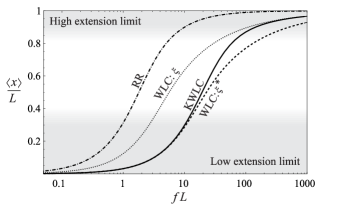
Figure 5: Force-extension characteristic for KWLC compared to WLC and Rigid Rod for $L=4\xi$ and $\zeta\xi=4$. At low extension, the force-extension of KWLC (solid curve) approaches WLC (dashed curve) with a persistence length equal to the effective persistence length of KWLC. At high extension, the kink modes are frozen out and the KWLC force-extension characteristic approaches WLC (dotted curve) with a persistence length equal to the bend persistence length of KWLC. Rigid Rod (dot dashed curve) has been plotted for comparison. The extension of Rigid Rod corresponds to alignment only.

In force-extension experiments, a single polymer molecule is elongated by a bead in an external field. The average extension of the polymer is measured as a function of external field strength. The forces opposing extension are entropic. These entropic forces are caused by the reduction in the number of available microstates as the polymer extension is increased. The persistence length defines the length scale on which the polymer tangents are correlated. For small persistence length, the number of statistically uncorrelated tangents is greater, which increases the size of the entropic contribution to the free energy relative to the external potential. This deceptively simple physics implies that a chain with a softer bending modulus acts as a stiffer entropic spring resisting extension.

To compute the force-extension relation, we must compute the partition function in an external field $f$ which can be concisely written in terms of the spatial partition function

$${\cal Z}_{\vec{f}}\ (L)=\int d^{3}x\ e^{\vec{f}\cdot\vec{x}}{\cal Z}(\vec{x};L)=\tilde{\cal Z}(i\vec{f};L),$$ (54)

which is a particularly convenient expression since it is the Fourier-transformed partition function with the wave number $\vec{k}$ analytically continued to $i\vec{f}$. Note that this is the inverse Laplace transform of eqn 45. The average extension is

$$\left<x(f)\right>=\frac{\partial}{\partial f}\log{\cal Z}_{\vec{f}},$$ (55)

which may be computed by taking the inverse Laplace transform numerically. (See Sect. A.2 for the numerical method.) The results are plotted in fig 5. In this figure, the KWLC theory interpolates between two WLC limits at high and low extension. The low-force limit is clearly related to low wave number limit (eqn 51) via an analytic continuation of the wave number. Therefore KWLC with effective persistence length $\xi^{*}$ and WLC with persistence length $\xi^{*}$ correspond in the low-extension limit as can be seen in fig 5.

At high force, fig 5 shows that kinking becomes irrelevant and the extension of KWLC and WLC both with bend persistence $\xi$ are identical. In this limit, the chain is confined to small deflection angles for which the effect of kinking is negligible, as can be seen in fig 3. In essence the kink modes freeze out and measurement of the extension versus force measures the bend persistence rather than the effective persistence length of the KWLC polymer chain.

These two regimes imply that in principle the value of $\zeta$ could be determined by the difference between the persistence length measured at small and large extension. In practice, this is most likely not practical. We have purposely chosen an unrealistically large value of $\zeta$ in fig 5, to illustrate clearly the low- and high-extension limits. In more realistic systems, the difference between the bend and effective persistence lengths would be small implying that it would be difficult to detect. Furthermore, at low extension the effects of polymer-polymer interactions can act to either increase or decrease the effective low extension persistence length. At high extension, polymer stretch also acts to increase the extension at high force most likely obscuring the effects of the entropy reduction due to the loss of the kink bending modes. Fig 6 illustrates these remarks.

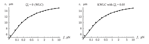
Figure 6: Left: Semilog plot of the best fit of the WLC model ($\zeta=0$) to experimental data on the force-extension relation of a single molecule of lambda DNA. Right: Best fit of the KWLC model to the same data, taking $\zeta\xi=0.05$. The fits are equally good, even though this value of $\zeta$ is larger than the one that we will argue fits cyclization data. Thus, force-extension measurements can only set a weak upper bound on the value of $\zeta$. (Data kindly supplied by V. Croquette; see Nelson (2004).)

The force-extension characteristic is therefore unlikely to detect the high-curvature softening induced by kinking.

V.3 Structure factor

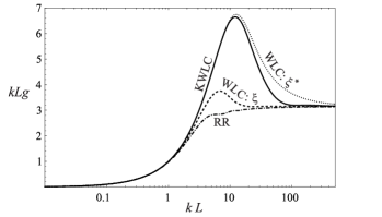
Figure 7: The structure factor and the role of effective persistence length. The solid curve is the structure factor for KWLC with contour length $L=4\xi$, and kink parameter $\zeta=4/\xi$. For comparison, we have plotted the structure factor for WLC of the same contour length for identical bend persistence lengths (dashed) and identical effective persistence length (dotted). At short length scales (large wave number) the KWLC structure factor approaches that for WLC with an identical bend persistence length. At long length scales (small wave number), the KWLC structure factor approaches that for WLC with a persistence length equal to its effective persistence length $\xi^{*}$. We have also plotted the structure factor for Rigid Rod (dot dashed curve) for comparison.

Another experimental observable used to characterize polymers is the structure factor, measured by static light scattering, small-angle X-Ray scattering, and neutron scattering experiments. Measurements of the structure factor can probe the polymer configuration on a wide range of length scales. Symbolically the structure factor is

$$g(\vec{k})\equiv\frac{1}{L^{2}}\int_{0}^{L}dsds^{\prime}\ \left<\exp\left[i\vec{k}\cdot\left(\vec{X}(s)-\vec{X}(s^{\prime})\right)\right]\right>,$$ (56)

where $\vec{X}(s)$ is the position of the polymer at arc length $s$ and we have included an extra factor of the polymer contour length in the denominator to make the structure factor dimensionlessSpakowitz and Wang (2004). At high wave number, the structure factor is sensitive to short length scale physics, whereas the polymer length and radius of gyration can be measured at low wave number. The structure factor can be rewritten in terms of the Laplace-Fourier transformed propagator

$$g(\vec{k})=\frac{2}{L^{2}}{\cal L}^{-1}\left[\frac{\tilde{K}(\vec{k};p)}{p^{2}}\right],$$ (57)

where ${\cal L}^{-1}$ is the inverse Laplace transform which can be computed numerically. (See Sect. A.2 for the numerical method.) As we mentioned above, the leading-order contributions at small wave vector are the polymer length and the radius of gyration

$$Lg(k)=L(1+{\textstyle\frac{1}{3}}\vec{k}^{2}R_{g}^{2}+...)$$ (58)

where we have temporarily restored the length dimension of $g$. At large $k$, both WLC and KWLC are rod-like or straight which gives an asymptotic limit for large wave number

$$g(k)\rightarrow\frac{\pi}{Lk},$$ (59)

since the chain is inflexible at short length scales.

To what extent can scattering experiments differentiate between WLC and KWLC? We have already argued that kinking merely leads to a renormalization of the persistence length for the radius of gyration, $R_{g}$, so both theories are identical at the low and high wave number limits. For the rest of the interval, the theories do predict subtly different structure factors, but for small values of $\zeta$, the theories are nearly indistinguishable. Again, we have chosen to illustrate the structure factor for an unrealistically large value of $\zeta$, to exaggerate its effect. Like force-extension measurements, scattering experiments are not sensitive to the high curvature physics since the signal is dominated by the thermally accessible bending regime which is essentially identical to WLC.

VI Cyclized chains and the $J$ factor

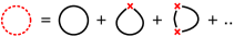
Figure 8: The diagrammatic representation of the kink number expansion for cyclized polymers. The dashed curve represents the KWLC theory which is the sum of the $m$ kink contributions. In the interval between the kinks, the polymer is described by WLC, represented by the solid curves. For each $m$ kink contribution, we sum over the kink position. In order to meet the tangent alignment conditions for cyclized polymers, we close the chain at a kink for kink number one or greater.

Although the theoretical study of the moment-bend constitutive relation is straightforward, it is problematic experimentally to apply a moment and measure the deflection directly on microscopic length scales. It is typically more convenient to let thermal fluctuations drive the bending, but as we have discussed above, experiments which measure thermally-driven bending are typically not sensitive to the rare kinking events. In contrast, cyclization experiments, although thermally driven, are sensitive to bending at any length scale. These experiments measure the relative concentrations of cyclized monomers to noncyclized dimers. By choosing the contour length of the monomers, any bending scale may be studied provided the concentration of cyclized molecules is detectable. Furthermore, these experiments are typically bulk rather than single molecule. In fact the data motivating this work comes from recent DNA cyclization measurements of Cloutier and WidomCloutier and Widom (2004) who have shown that the cyclization probability is $10^{4}$ to $10^{5}$ times larger than that predicted by WLC for DNA sequences with a contour length $L\approx 0.6\xi$, while confirming that larger sequences ($L>\xi$) do cyclize at the rate theoretically predicted by the WLC

In cyclization measurements, the configurational free energy is isolated in the $J$ factor which is ratio of the cyclization equilibrium constant to the dimerization equilibrium constantJacobson and Stockmayer (1950). This ratio eliminates the dependence on the end-end interaction free energy. For non-twist storing polymers, the $J$ factor is proportional to the tangent-spatial propagatorJacobson and Stockmayer (1950)

$$J=4\pi G(0;\vec{t},\vec{t};L),$$ (60)

which is the concentration of one end of the polymer chain at the other ($\vec{x}=0$) with the correct tangent alignment. The factor of $4\pi$ is due to the isotropic angular distribution of monomer in free solution. Our analysis will neglect additional complications relevant to the study of real DNA. First, in DNA the twist must also be aligned, which requires the use of a variant of WLC, Helical Wormlike ChainYamakawa (1997). This additional constraint modulates the $J$ factor with a 10.5 bp period equal to the helical repeat. Our interest here is in the value of the $J$ factor averaged over a helical repeat for which the effects of twist can be roughly ignoredYamakawa (1997). A second complication in real DNA is sequence dependent prebendingManning et al. (1996); Zhang and Crothers (2003). We argue elsewhere that prebending effects alone cannot explain the high cyclization rates observed for short DNAWiggins et al. (2004); in this paper we focus instead on kink formation.

Although cyclization experiments are fairly straightforward, extracting mechanical information from the results poses a difficult theoretical problem due to the combination of tangent and spatial constraints. In fact, there is no exact analytic expression for the $J$ factor in the WLC theory; the following sections and appendices will develop the numerical methods we need.

VI.1 The looping $J$ factor

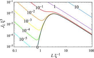
Figure 9: The KWLC looping $J$ factor, $J^{*}_{L}$, as a function of contour length plotted for various values of the kinking parameter $\zeta$. The numbers labeling the curves indicate the value of the dimensionless quantity $\xi\zeta$. WLC is the curve labeled 0. For large contour length $L$, the effect of kinking can be accounted for by computing $J_{L}$ for the effective persistence length, $\xi^{*}$. But as the contour length shrinks to a persistence length, the effect of kinking becomes dominant, even for small $\zeta$. At short contour length the looping $J$ factor is one kink dominated and diverges in contrast to the WLC looping $J$ factor which approaches zero precipitously for short contour length.

Due to these computational complications, we shall initially dispense with the tangent alignment condition and compute a modified $J$ factor that is relevant for processes that do not fix the tangents of the chain. For example some protein-DNA complexes exhibit a behavior that is believed to be better represented by looping (free end tangents) than cyclization (end tangents aligned) Zhang et al. (2004). We define the looping $J$ factor as the ratio of the looping to the dimerization equilibrium constants. The KWLC looping $J$ factor, $J^{*}_{L}$, can be written in terms of the spatial propagator as

$$J_{L}^{*}=K^{*}(0;L),$$ (61)

which can be interpreted as the concentration of one end at the other. We have again neglected the effect of twist. In this case the explicit $4\pi$ in eqn 60 is not needed, as the definition of $K$ already includes an integral over angles. Both from the standpoint of developing intuition and computational convenience it is useful to explicitly expand $K^{*}$ in the kink number. We introduce the WLC closed spatial propagator convolutions which we denote

$${\cal K}^{(m)}\equiv\left[K\otimes\right]^{m}(0;L),$$ (62)

where again the $\otimes$ represents both spatial and arc length convolutions. The computation of the ${\cal K}^{(m)}$ is discussed in section A.3. In terms of the ${\cal K}^{(m)}$, the free tangent $J$ factor is

$$J_{L}^{*}=e^{-\zeta L}\sum_{m=0}^{\infty}\zeta^{m}{\cal K}^{(m+1)},$$ (63)

where we have defined the ${\cal K}^{(m)}$ to be independent of the kinking parameter $\zeta$. The kink number sum is illustrated with a diagrammatic expansion in fig 8. The probability of the $m$ kink state can be concisely written in terms of the ${\cal K}^{(m)}$

$${\cal P}_{m}=e^{-\zeta L}\zeta^{m}\frac{{\cal K}^{(m+1)}}{J_{L}^{*}}.$$ (64)

This expression can be interpreted as the kink number distribution for a looped chain, a constraint that induces kinking in a manner roughly analogous to the tangent constraints already discussed in detail. The looping $J$ factor is plotted in fig 9. In this figure, we can see that the intuition we developed computing the moment-bend constitutive relation is borne out in the looping $J$ factor, despite the fact that the process is thermally driven. In the short-length limit, the ability of the chain to kink dramatically reduces the bending energy and increases the looping $J$ factor. In the short-length limit, a single kink is nucleated in a manner almost exactly analogous to the process we have described in detail for the moment-bend constitutive relation. We will discuss these results and their scaling in more detail after computing the KWLC $J$ factor.

VI.2 The cyclization $J$ factor

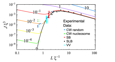
Figure 10: (Color.) The KWLC cyclization $J$ factor as a function of contour length $L$ for various values of the kink parameter $\zeta$. As discussed in the text, our theory does not include the twist induced 10.5 bp modulation of the $J$ factor. The numbers labeling the curves indicate the value of the dimensionless parameter $\xi\zeta$. The WLC theory corresponds to $\zeta=0$. For large contour length $L$, the effect of kinking can be accounted for by computing the $J$ factor using the effective persistence length, $\xi\zeta$. As the contour length $L$ falls below a persistence length, kinking dramatically increases the $J$ factor, even for small $\zeta$. For small $L$ the chain is two kink dominated and diverges, in contrast to the WLC theory which precipitously falls to zero at small $L$. Experimental cyclization data for DNA are plotted for comparison, assuming $\xi=50$ nm. (Data sources: CWCloutier and Widom (2004), SBShore and Baldwin (1983), SLBShore et al. (1981), and VVVologodskaia and Vologodskii (2002).) At contour length $L=0.6\xi$, the experimentally measured $J$ factor is $\approx 10^{4}$ times larger than predicted by the WLC theoretical curve. The KWLC with $\zeta\xi=10^{-2}$ correctly captures this behavior, while matching the WLC theory at large contour length.

Although the computation of the free tangent $J$ factor is more direct and intuitive, the $J$ factor with tangent alignment is of more phenomenological interest. The computation begins with the tangent-spatial partition function defined in eqn 45 for end distance zero and aligned tangents. Since the transformed WLC tangent-spatial propagator is unknown, it would initially appear to preclude exploiting the exact results derived above. But intuitively we know the chain may be closed at any point resulting in an identical $J$ factor. For kinked chains, it is convenient to close the chain at a kink where the tangent alignment condition is no longer required. The only chains for which this simplification cannot be applied are the unkinked chains for which the $J$ factor is already knownShimada and Yamakawa (1984). To show this explicitly, we write the transform of Eqn. 45 in its expanded form and specialize to $\vec{t}=\vec{t}_{0}$ to obtain the cyclization partition function:

$${\cal Z}^{*}_{C}(L)=G(0;\vec{t},\vec{t};L)+\sum_{m=0}^{\infty}\left(\zeta G^{\prime}(\vec{t}\ )\otimes\left(\zeta K\otimes\right)^{m}G^{\prime}(\vec{t}\ )\right)(0;L).$$ (65)

We can now use the composition property of the propagators to replace the initial and final tangent-spatial propagators with a single spatial propagator. Some care is now required in performing the convolution, as described in appendix A.1. The cyclization partition function then becomes (Eqn. 87)

$${\cal Z}_{C}^{*}(L)=G(0;\vec{t},\vec{t};L)+\frac{1}{4\pi}\sum_{m=1}^{\infty}\frac{\zeta^{m}L}{m}{\cal K}^{(m)},$$ (66)

where we have expressed the result in terms of the zero end distance spatial propagator convolutions, ${\cal K}^{(m)}$. The kink number sum is illustrated with a diagrammatic expansion in fig 8. This equation has an analogous form to the looping $J$ factor in Eqn. 63. The only complication here is that for kinked chains, the state counting has subtly changed since we close the chain at a kink. For inverse transform numerical computations, it is convenient to write a transformed partition function

$$\tilde{\cal Z}_{C}^{*}(k;p)=\tilde{G}+\frac{1}{4\pi}\frac{\partial}{\partial p}\log\left[1-\zeta\tilde{K}\right],$$ (67)

although the expression is understood to only have physical meaning when the chain is closed ($\vec{x}=0$). Our derivation of the cyclized partition function implies that the KWLC tangent-spatial propagator is known for one special case

$$G^{*}(0;\vec{t},\vec{t};L)=e^{-\zeta L}{\cal Z}_{C}^{*}(L),$$ (68)

which is precisely the expression we need to compute the $J$ factor. In terms of the KWLC tangent-spatial propagator, the KWLC $J$ factor is

$$J^{*}=4\pi G^{*}(0;\vec{t},\vec{t};L)=e^{-\zeta L}\sum^{\infty}_{m=0}\zeta^{m}{\cal J}^{(m)},$$ (69)

where we have explicitly expanded the $J$ factor in kink number. The ${\cal J}^{(m)}$ are defined by

$${\cal J}^{(m)}\equiv\begin{cases}J,&m=0\\ Lm^{-1}{\cal K}^{(m)},&m>0\end{cases}.$$ (70)

Fig 10 compares experimental data to our theoretical calculation of $J^{*}$. Details of the calculation are discussed in appendix A.3. Note that setting the kink density to $\zeta\approx 10^{-2}/\xi=0.2/\mu$m roughly reproduces the experimental cyclization data. Eqn 7 connects $\zeta$ to the density of vertices $\ell$ and the free energy cost $\epsilon$ of creating a kink. Assuming that the site density is just the DNA base pair length $\ell=0.34\,$nm, we can estimate the kink energy,

$$\epsilon=\ln\left[\frac{2\xi}{\ell^{2}\zeta}\right]\approx 15\ kT\approx 9\,\mbox{kcal/mol}\ .$$ (71)

Although we do not discuss detailed microscopic models in this paper, it is interesting to note that molecular modeling studies have found that in B-form DNA, base pairs indeed open individually and noncooperatively with an activation energy of 10–20kcal/mol Bernet et al. (1997).

VI.3 Topologically induced kinking

It is useful to discuss kink number in chains that are topologically confined to be cyclized. These chains have both the kink inducing tangent and spatial constraint.

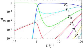
Figure 11: The kink-number distribution compared for cyclized chains (solid curves) and unconstrained chains (dashed curves) as a function of contour length $L$. To illustrate constraint-driven kinking, we have chosen the illustrative value $\zeta\xi=10^{-2}$. At large contour length $L$, the cyclization constraint is irrelevant but as the arc length shrinks to roughly a persistence length, the bending energy required to cyclize the chain becomes significant and there is a dramatic transition to the two kink state which dominates at short contour length. The contributions of one and $m>2$ kink states are secondary.

We can write the kink number distribution concisely in terms of the $J$ factor

$${\cal P}_{m}=e^{-\zeta L}\zeta^{m}\frac{{\cal J}^{(m)}}{J^{*}},$$ (72)

which is analogous to eqn 64 and depicted in fig 11.

The effects of kinking on the $J$ factor are dramatic even when the kinking parameter $\zeta$ is small! Fig 10 shows that the WLC $J$ factor precipitously decreases with loop contour length due to the increasing elastic energy required to close the loop:

$$J\sim e^{-2\pi^{2}\xi/L}.$$ (73)

In dramatic contrast, the KWLC $J$ factor, while tracking the WLC $J$ factor at large contour length, turns over at small contour length and increases divergently. Physically, this small contour length divergence can be understood as an increase in the ratio of available cyclized to noncyclized states which is roughly inversely proportional to the physical volume explored by the chain when one end is fixed. This divergent increase in the density of states can also be seen for the Gaussian Chain in the short length limit, although this limit is not physical for polymer systems. For the Gaussian chain, the $J$ factor is monotonically decreasing with contour length since the only obstruction to the ends finding each other is entropic, and the number of available noncyclized states scales like $L^{3/2}$ (eqn 104). For KWLC, once the chain is kinked twice, it is advantageous to shorten the chain which, while decreasing the degeneracy of the first kink location, $\propto L$ (eqn 70), increases the density of cyclized states, $\propto L^{-2}$ (eqn 95). Therefore, there is a net $L^{-1}$ scaling of the two kink term ${\cal J}^{(2)}$ (eqn 70). In this limit, the contributions from chains with kink numbers greater than two scale like $L^{m-3}$ (eqns 70 and 102), implying that at short lengths the two kink term dominates. In addition, in most physically interesting scenarios the kinking parameter $\zeta$ is small. The probability of $m$ kink number state scales roughly like the average kink number for the unconstrained chain to the $m$th power $(L\zeta)^{m}$ (eqn 69), which further decreases the importance of higher kink number states. The dramatic transition from the zero kink to the two kink state at short contour length is evident in fig 11. Interestingly, recent molecular-dynamics simulations on a 94 bp DNA minicircle indicate the presence of two sharply kinked regions lav (2004).

Physically, we can understand the onset of this transition by roughly comparing the free energies of the two kink term and the zero kink term to find the length at which these two are roughly equal. Here we merely wish to motivate our results as clearly and simply as possible so we shall ignore the difference in the density of states, even though its effect is quantitatively important. We therefore treat the free energy of the zero kink term as the bending energy only and the free energy of the two kink term as twice the kink energy in the discrete model (eqn 7):

$$2\epsilon\sim\frac{2\pi^{2}\xi}{L_{\rm crit}}.$$ (74)

When the bending energy equals the energy required to nucleate two kinks, the transition occurs. It is important to remember that the $\zeta$-dependence is relatively weak while the bending energy scales like the inverse of the contour length. Below $L\sim\xi$, the bending energy grows divergently implying that even for very small kink densities, kinking always becomes important at short enough contour length. That is to say, we are almost assured of observing elastic breakdown effects below contour lengths of roughly a persistence length.

Previously we had shown that for moment-bending, only a single kink was nucleated, in contrast to the current example where the one kink contribution to the $J$ factor, ${\cal J}^{(1)}$, is of little scaling importance since the chain must still bend as illustrated schematically in fig 8. This will not be the case for the KWLC looping $J$ factor, $J_{L}^{*}$, which lacks the tangent constraint implying that only one kink is required to relieve all the elastic bending. The one kink term of $J_{L}^{*}$ therefore diverges like $L^{-2}$ (eqn 95) as explained above. $J_{L}^{*}$ is plotted in fig 9.

VII Discussion

Our main results are summarized in figs 5, 6, 10, and 11. We formulated a generalization of the WLC model, in which a semiflexible polymer can develop flexible sites of an alternative conformation. We found that taking the density of kinks in the unstressed polymer to be about $0.01$ per persistence length has negligible effect on the force–extension relation, but vastly enhances the probability of cyclization for chains shorter than a persistence length, as seen in recent experiments on DNA Cloutier and Widom (2004).

Various microscopic mechanisms could furnish the kinking mechanism in DNA, for example single-basepair flipout or strand separation Wiggins et al. (2004). But any complete, microscopic analysis of high-curvature DNA conformations would also have to include a variety of effects, for example those arising from the significant thickness of the DNA molecule on the few-nanometer scale of a short circle, strong polyelectrolyte effects, and so on. We have taken the attitude that any net nonlinear softening at high curvature will lead to generic new phenomena. By summarizing all such effects into a single phenomenological parameter, our model focuses attention on the general mesoscale physics of kinking. The KWLC’s generality also makes it a useful starting point for studying the conformations of other stiff biopolymers, such as actin.

Other diagnostics of low-curvature physics, for example light scattering, also turned out to be almost indistinguishable from the linearly-elastic Wormlike Chain model. It is only by conducting experiments that are explicitly sensitive to high curvature, that we can measure the nonlinear response to bending. DNA cyclization offers one experimentally tractable measurement sensitive to the high-curvature physics of free DNA in solution; we gave predictions for other, future tests, for example the moment–bend relation and the kink number as a function of constraints. Indeed, the predicted average number of kinks has direct structural implications for very small DNA loops, and for processes involving such loops, for example, the looping implicated in some gene-regulatory mechanisms Bellomy et al. (1988); Rippe et al. (1995); Muller et al. (1996, 1998); Rippe (2001); Zhang et al. (2004). Recent simulations indeed suggest that spontaneous kinking may play a role in such situations lav (2004).

Some mathematical aspects of the model, for example the divergence of the theoretical $J$ factor at small contour length (fig 10), are artifacts of the simplified picture we have proposed. The small contour length divergence is due to the two kink term, which can close a loop without elastic bending regardless of the contour length, via the creation of 180-degree kinks! Clearly due to the finite thickness of the chain, this divergence is unphysical. We can consider a number of modifications to the theory to fix this problem: kink angle cutoffs, kinks that are not perfectly flexible, etc. But all these proposals require adding additional parameters to the model, rendering it both less tractable and less predictive, since the additional parameter must then be fit to experimental data.

The KWLC is in essence a coarse-grained, effective theory for systems where kinking occurs and the kinks are localized compared with the chain persistence length. Its virtue is that it offers a simple way to characterize stiff biopolymers, and a quantitative guide to the mesoscale effects of kinking. Thanks to this simplicity, we were able to compute many results in this paper exactly, without extensive numerical simulation. We discuss the specific application of KWLC to DNA at length elsewhereWiggins et al. (2004).

Appendix A Fourier & Laplace Transforms & convolution theorems

The relations listed below are well knownArfken and Weber (1995) but essential to our derivations. We define the 3D spatial Fourier Transform and inverse transform

$$\tilde{F}(\vec{k}) \equiv {\cal F}\{F(\vec{x})\}=\int d^{3}x\ F(\vec{x})e^{-i\vec{k}\cdot\vec{x}},$$ (75)

$$F(\vec{x}) = {\cal F}^{-1}\{\tilde{F}(\vec{k})\}=\left(\frac{1}{2\pi}\right)^{3}\int d^{3}k\ \tilde{F}(\vec{k})e^{i\vec{k}\cdot\vec{x}}.$$ (76)

The Faltung theorem states that Fourier Transform of a convolution is the product of the Fourier Transforms:

$${\cal F}\{F\otimes G\}=\tilde{F}\tilde{G},$$ (77)

for functions $F$ and $G$ where the spatial convolution is defined

$$F\otimes G(\vec{x})\equiv\int d^{3}x^{\prime}\ F(\vec{x}{\,}^{\prime})G(\vec{x}-\vec{x}{\,}^{\prime}).$$ (78)

The generalization of the Faltung theorem is true for $n$ functions

$${\cal F}\{F_{1}\otimes...\otimes F_{m}\}=\tilde{F}_{1}...\tilde{F}_{m}.$$ (79)

We define the 1D contour length Laplace Transform and inverse transform

$$\tilde{F}(p) \equiv {\cal L}\{F(L)\}=\int^{\infty}_{0}dL\ F(L)e^{-pL},$$ (80)

$$F(L) = {\cal L}^{-1}\{\tilde{F}(p)\}=\frac{1}{2\pi i}\int_{\cal L}dp\ \tilde{F}(p)e^{pL},$$ (81)

where $\int_{\cal L}$ denotes a contour integral along the Laplace contour. The Faltung theorem states that Laplace Transform of a convolution is the product of the Laplace Transforms:

$${\cal L}\{F\otimes G\}=\tilde{F}\tilde{G},$$ (82)

for functions $F$ and $G$, where the arc length convolution is defined

$$F\otimes G(L)\equiv\int_{0}^{L}dL^{\prime}\ F(L^{\prime})G(L-L^{\prime}).$$ (83)

The generalization of the Faltung theorem is true for $m$ functions

$${\cal L}\{F_{1}\otimes...\otimes F_{m}\}=\tilde{F}_{1}...\tilde{F}_{m}\ .$$ (84)

A.1 Circular convolutions

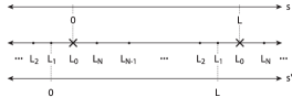
Figure 12: A schematic diagram of the coordinate transformation exploited to compute the circular convolution. The crosses represent chain ends and dots represent kinks. The center line represents a periodic coordinate system. For regular convolutions, we set the chain end to be the zero and we compute the convolution in the $s$ coordinate system. For the circular convolution, it is more convenient to choose $L_{1}$, the first kink arc length position as the zero and sum over the chain end positions as represented by the $s^{\prime}$ coordinate system.

For the closed chain we need to evaluate a special type of convolution which is circular. By circular we mean that the end points are identified so that the arc-length position of the chain ends is not at an end point of the propagator. In this case it is convenient to redefine the arc-length coordinate system to be zero at the position of the first kink, $L_{1}$, and sum over the position of the chain ends as depicted in fig 12. The $m$ kink contribution to the partition function is therefore

$${\cal Z}_{m}^{*}=\frac{\zeta^{m}}{4\pi}\left[\left(K\otimes\right)^{m-1}LK\right](0;L),$$ (85)

where the factor of $L$ comes from the integration over the end position and varies in the convolution. To simplify this result it is convenient to go to the transformed partition function

$$\tilde{\cal Z}_{m}^{*}=-\frac{\zeta^{m}}{4\pi}\tilde{K}^{m-1}\frac{\partial}{\partial p}\tilde{K}=-\frac{\zeta^{m}}{4\pi m}\frac{\partial}{\partial p}\tilde{K}^{m},$$ (86)

where the $L$ has been transformed into a $p$ derivative. We now return from Fourier-Laplace space, giving:

$${\cal Z}_{m}^{*}=\frac{\zeta^{m}L}{4\pi m}\left[K\otimes\right]^{m}(0;L),$$ (87)

which is written in terms of convolutions of the spatial propagator only.

A.2 Numerical inverse transforms

To compute the numerical inversions of the Fourier and Laplace Transforms involving the spatial propagator, we first truncate the continued fraction Spakowitz and Wang (2004) in eqn 49, then we compute the numerical inversion with the built-in Mathematica functions InverseLaplaceTransform and InverseFourierTransform. In particular, the structure factor and partition function in an external field involve only a single numerical inverse Laplace Transform.

A.3 $J$ factor computation

We have chosen to present most of our results in the last section as explicit series in kink number rather than writing them in the summed form (eqn 48 and 67). The purpose is two fold. First these expansions allow $J$ to be computed efficiently for many small values of $\zeta$, because the ${\cal K}^{(m)}$ are independent of $\zeta$ and only the first few must be computed explicitly for sufficient numerical accuracy. Furthermore the ${\cal K}^{(m)}$ are simply related to the kink number distribution allowing the same computation to suffice for both results. Our computational discussion will mainly focus on the short contour length limit where these kink number expansions converge quickly. As we have already discussed at length, the large contour length limit can trivially be computed with the WLC results using the renormalized effective persistence length, $\xi^{*}$. This corresponds to the $k\rightarrow 0$ and $p\rightarrow 0$ limit where the theories are identical. In fact, in this limit, we can use the Gaussian chain to compute the $J$ factor. This computation appears briefly in appendix C.

It is at short contour length where the two theories significantly diverge and kinking is induced. As we have discussed above, in the limit as the contour length goes to 0, the polymer resembles a rigid rod. It is problematic to directly compute the inverse transforms of $K^{*}$ or $K$ numerically in this limit since

$$K(0;L\rightarrow 0)\propto\int^{\infty}_{0}dk\ k\sin kL,$$ (88)

which, although it can be computed analytically by expanding sine into two exponentials then integrating them on different contours, is problematic numerically. It is therefore convenient to use the expanded definition of $K^{*}$ in terms of the ${\cal K}^{(m)}$ (eqn 62). In the short contour length limit, an asymptotic expression already existsYamakawa (1997) for $J$ and $K(0;L)$.

Convolutions of $K$ must still be computed. Numerical computations of the inverse transforms of powers of $\tilde{K}$ are still problematic in the $L\rightarrow 0$ limit since, while they are more convergent than $K$, they must be integrated to large $k$ where it is difficult to compute accurate Laplace transforms. But this implies it is in precisely this limit that bending is really irrelevant and that the mechanics of these kinked chains becomes kink dominated. Once there are two or more kinks, the chain can now be closed without elastic bending. That is to say that, when these terms become difficult to calculate numerically, they can be well approximated by the kinkable rigid rod! The kinkable rigid rod is treated in appendix B. As a practical matter there is a small contour length regime ($L\sim 1$), between the rigid rod limit and the contour length at which numerical transform inversion are rapidly convergent and where it is most convenient to use direct Monte Carlo integrations to compute the ${\cal K}^{(m)}$. These direct Monte Carlo integrations serve as a useful check on our other numerical and analytic computations. For large dimensionless kink densities, the kink-number expansion is not rapidly converging and direct numerical inversions of the exactly summed transformed results are required. For most computations of the $J$ factor at small kink density, the rigid rod approximation suffices to compute the two kink term and the kink number sum can be truncated at this point as illustrated schematically by Fig 11.

Appendix B Kinkable rigid rod

In this section we develop the theory of kinkable rigid rods, the infinite persistence length limit of the KWLC. This theory is useful for discussing the short loop limit of the $J$ factor. The rigid rod tangent-spatial propagator is

$$G(\vec{x},\vec{t}_{L},\vec{t}_{0},L)=\delta^{(3)}\left[\vec{x}-L\vec{t}_{L}\right]\ \delta^{(2)}\left[\vec{t}_{L}-\vec{t}_{0}\right].$$ (89)

The spatial propagator, $K$, is obtained by averaging and summing over the two tangents (eqn 41)

$$K(\vec{x},L) = \frac{1}{4\pi L^{2}}\delta\left[|\vec{x}|-L\right].$$ (90)

The Fourier and Fourier-Laplace transform spatial propagator are

$$\tilde{K}(\vec{k},L) = \frac{\sin kL}{kL},$$ (91)

$$\tilde{K}(\vec{k},p) = \frac{1}{k}\tan^{-1}\frac{k}{p}.$$ (92)

In order to discuss the $J$ factor limit, we will need the convolutions

$${\cal K}^{(m)}\equiv[K\otimes]^{m}(0,L),$$ (93)

which is proportional to the probability density of the end distance be $0$ after arc length $L$ and $m-1$ kinks. ${\cal K}^{(1)}$ is zero since the rod is rigid and the ends cannot meet unless the chain kinks.

${\cal K}^{(2)}$ is also fairly straight forward. It is convenient to compute the convolution explicitly

$${\cal K}^{(2)} = \frac{1}{2\pi^{2}}\int^{L}_{0}dL_{1}\int^{\infty}_{0}dk\ k^{2}\ \frac{1}{kL_{1}}\sin kL_{1}\ \frac{1}{k(L-L_{1})}\sin k(L-L_{1})$$ (94)

$$= \frac{1}{2\pi L^{2}},$$ (95)

where the Fourier transform delta function has been used to evaluate the integral.

The computation of ${\cal K}^{(3)}$ requires some care. Again it is convenient to compute the convolution explicitly

$${\cal K}^{(3)} = \frac{1}{2\pi^{2}}\int^{L}_{0}dL_{1}\int^{L}_{0}dL_{2}\int^{L}_{0}dL_{3}\ \int^{\infty}_{0}dk\ k^{2}\ \times$$ (96)

$$\frac{1}{kL_{1}}\sin kL_{1}\ \frac{1}{kL_{2}}\sin kL_{2}\ \frac{1}{kL_{3}}\sin kL_{3}\ \delta\left(L_{1}+L_{2}+L_{3}-L\right),$$

$$= \frac{1}{8\pi^{3}}\int^{L/2}_{0}dL_{1}\int^{L/2}_{L/2-L_{1}}dL_{2}\frac{1}{(L-L_{1}-L_{2})L_{1}L_{2}},$$ (97)

$$= \frac{\pi}{16L}.$$ (98)

For convolution number $m>3$, we exploit the Fourier-Laplace transform method

$${\cal K}^{(m)} = \frac{1}{2\pi^{2}}\int^{\infty}_{0}dk\ k^{2}\int_{\cal L}dp\ \left(\frac{1}{k}\tan^{-1}\frac{k}{p}\right)^{m}e^{pL}$$ (99)

$$= \frac{1}{2\pi^{2}}\int^{\infty}_{0}dk^{\prime}\ {k^{\prime}}^{2}\int_{\cal L}dp\ p^{3-m}\left(\frac{1}{k^{\prime}}\tan^{-1}k^{\prime}\right)^{m}e^{pL},$$ (100)

where we have made the substitution $k^{\prime}=k/p$. Now let us compute the $k^{\prime}$ integral, which must be done numerically. We now make the substitution $\tan x=k^{\prime}$. The integral in $k^{\prime}$ becomes

$$I_{m}\equiv\frac{m}{m-3}\int^{\pi/2}_{0}dx\tan^{3-m}x\ x^{m-1},$$ (101)

which we computed using Mathematica.

convolution	Integral
number $m$	$I_{m}$
4	2.249
5	0.841
6	0.461
7	0.300
$\cdots$	$\cdots$

Table 1: Values for the numerically computed integral $I_{m}$ for the first few $m$.

The $p$ integral is now a simple contour integral which gives

$${\cal K}^{(m)} = \frac{I_{m}}{2\pi^{2}}\frac{L^{m-4}}{(m-3)!},$$ (102)

for $m>3$. The first few values of $I$ are computed numerically in table 1.

The kinkable rigid rod theory, derived above, provides a very useful analytic check of the KWLC model at short contour length. For short cyclized polymers, the bending between kinks can be ignored since these segments are significantly shorter than a persistence length. As we have illustrated above, the computation of the dominant two kink contribution is straightforward in this limit.

Appendix C Gaussian limit

The Gaussian limit provides a useful analytic limit to the KWLC theory for long contour length. In this limit, the length of the polymer makes the initial tangent condition irrelevant and describes the spatial distribution for chain extensions short compared with the contour length.

For large $L$, we can work with the Gaussian distribution. The Gaussian distribution is

$$G(\vec{x};\vec{t},\vec{t}{\ }^{\prime};L)=\frac{1}{4\pi}\left(\frac{3}{4\pi\xi L}\right)^{3/2}\exp\left[-\frac{3\vec{x}^{\,2}}{4\xi L}\right]$$ (103)

for persistence length $\xi$. The $J$ factor is

$$J=4\pi G(0;\vec{t},\vec{t};L)=\left(\frac{3}{4\pi\xi L}\right)^{3/2}.$$ (104)

For KWLC, the persistence length is replaced by the effective persistence length $\xi^{*}$:

$$J^{*}=4\pi G^{*}(0;\vec{t},\vec{t};L)=\left(\frac{3}{4\pi{\xi^{*}}L}\right)^{3/2}.$$ (105)

In the Gaussian limit, the convolution functions ${\cal K}^{(m)}$ can be computed without difficulty:

$${\cal K}^{(m)}=\frac{L^{m-1}}{(m-1)!}\left(\frac{3}{4\pi\xi L}\right)^{3/2}.$$ (106)

But this expression holds only when the number of kinks is small.

Appendix D Summary of notation

We imagine a chain of total contour length $L$, with $L/\ell$ elementary segments of length $\ell$. Individual segments will be referred to by their sequence number $n=0,\ldots N$, where $N=(L/\ell)-1$, or by arclength $s=n\ell$. A configuration $\Gamma$ consists of a sequence of tangent vectors $\{\vec{t}_{0},\ldots,\vec{t}_{N}\}$.

The stiffness parameter (WLC persistence length) $\xi$, one-vertex partition function $Q$, kink formation energy $\epsilon$, and kinking parameter $\zeta$ are defined in Sects. II–III. $\xi^{*}$ and $Q^{*}$ are related quantities relevant to the KWLC. The kink length is $\xi_{\rm kink}\equiv\zeta^{-1}$.

The measure $d^{2}\vec{t}\,$ denotes solid angle on the sphere of unit vectors $\vec{t}$. Square brackets denote the functional measure $[d\vec{t}\,(s)]_{\vec{t}_{\rm i}}\,$; see eqn 8.

The partition functions ${\cal Z}(L)$ and ${\cal Z}(\vec{t}_{\rm f},\vec{t}_{\rm i};L)$ refer to unconstrained and constrained functional integrals over a chain of length $L$ in the continuum limit. Rotation invariance implies that the constrained function depends only on the angle $\theta$ between the vectors, so we sometimes write it as ${\cal Z}(\theta;L)$. Discretized versions of the partition functions are denoted with the subscript “discrete,” and KWLC versions with a star. Related quantities include the free energy $F(\theta;L)=-\log{\cal Z}(\theta;L)$ (eqn 28) and the normalized tangent partition function (or propagator) $H(\vec{t}_{\rm f},\vec{t}_{\rm i};L)={\cal Z}(\vec{t}_{\rm f},\vec{t}_{\rm i};L)/{\cal Z}(L)$. Laplace transforms of these functions on $L$ are denoted with a tilde.

When it is important to maintain spatial information, we introduce space-dependent functions ${\cal Z}(\vec{x},\vec{t}_{\rm f},\vec{t}_{\rm i};L)$ (eqn 40), $K(\vec{x};L)$ (eqn 41), and $G^{\prime}(\vec{x},\vec{t};L)$ (eqn 42). Fourier–Laplace transforms of these functions on $\vec{x},L$ are again denoted with a tilde.

Laplace and Fourier transformations, and the corresponding convolution operation $\otimes$, are defined in appendix A. Repeated convolutions of $K$ give the functions ${\cal K}^{(m)}$ (eqn 62), and the related ${\cal J}^{(m)}$ (eqn 70).

The partition function in an external force is ${\cal Z}_{\vec{f}}$ (eqn 54); the cyclization partition function is ${\cal Z}^{*}_{C}(L)$ (eqn 65).

In an expansion in kink number, $m$ labels the number of kinks and $i=1,\ldots,m$ labels which kink is in question. The kinks are taken to be located at $n_{i}$, or at arc length position $L_{i}=\ell n_{i}$.