Time-dependent local Green’s operator
and its applications to manganites

Abstract

An algorithm is presented to calculate the electronic local time-dependent Green’s operator for manganites-related hamiltonians. This algorithm is proved to scale with the number of states $N$ in the Hilbert-space to the 1.55 power, is able of parallel implementation, and outperforms computationally the Exact Diagonalization (ED) method for clusters larger than 64 sites (using parallelization). This method together with the Monte Carlo (MC) technique is used to derive new results for the manganites phase diagram for the spatial dimension D=3 and half-filling on a 12x12x12 cluster (3456 orbitals). We obtain as a function of an insulating parameter, the sequence of ground states given by: ferromagnetic (FM), antiferromagnetic AF-type A, AF-type CE, dimer and AF-type G, which are in remarkable agreement with experimental results.

I Introduction

The doped manganites are interesting not only because of the potential applications of their ’colossal’ properties, but also because they are fascinating systems to study due to the delicate balance of interactions between charge, spin, and orbital degrees of freedom.kaplan

One of the successful theoretical approaches to the study of the manganites phase diagrams, is based on effective models that consider the competition between double-exchange (DE), superexchange (SE), and the electron-phonon interactions1 . These models and techniques have predicted interesting phenomena, like nanoscale phase-separation2 , influence of disorder in metal-insulator transitions3 , and the existence of non-trivial magnetic phases4 , among other phenomena. The ground states of such systems and the finite-temperature properties were obtained using simulations on clusters of spins using the Monte Carlo (MC) technique together with the calculation of the electronic energies by means of the exact diagonalization (ED) technique2 at each single MC step. In order to extract useful information from the simulations, one needs to analyze different sizes for the clusters, where the CPU (Central Processing Unit) memory and time scale as the number of states $N$ in the Hilbert space to the third- and fourth-power, respectively. In 1999, the Truncated Polynomial Expansion (TPEM)motome1 was devised in order to reduce the CPU time scaling with $N$, but unfortunately at a cost of a large prefactor and a detailed comparison with exact case (ED) was not shown.

Moreover, it is of fundamental importance to consider the Mn-$e_{g}$ orbitals $d_{x^{2}-y^{2}}$ and $d_{3z^{2}-r^{2}}$ at each sitekaplan , which doubles the size of the matrices respect of the case of a single band. The ED operations have to be performed several thousands times in a typical simulation, practically limiting the spatial dimensions of the clusters considered to D=1 and 2. The reduction in the dimensionality of the system artificially breaks the degeneracy of the orbitals $d_{x^{2}-y^{2}}$ and $d_{3z^{2}-r^{2}}$, modifying the electronic properties of the system.

For all these reasons it is important to find an alternative way to calculate the electronic energy that avoids the natural limitations of the ED scheme, allowing to expand the size of the clusters and the spatial dimensionality. An efficient and fast way to calculate the time-dependent Green’s operator in an effective model conceived for manganites will be described in this work. This method uses the Chebyshev expansion of the time evolution operator5 which is an extremely accurate and fast way to obtain the dynamics response of quantum many-body systems. For a system consisting of 10 spins S=1/2 with Heisenberg-like interactions, this expansion is three orders of magnitude faster than the ED method, and for a variety of considered cases, is one of the most efficient time-marching schemes to keep track of the time evolution of a quantum system, where CPU memory and time basically scale linearly with system size.5

In this work we will focus our attention to non-trivial single-particle Hamiltonians, where the Hilbert space grows linearly with the size of the system. More generally speaking, the presently described method, which will be referred as the Dyn method, provides an alternative way to calculate the local time-dependent Green’s operator for the time-dependent Schrödinger equation (TDSE). The Chebyshev expansion of the hermitian, time-independent, differential Hamiltonian operator $H$ will be applied to a model related to manganites, which is more efficient than the ED technique for electronic clusters larger than 64 orbitals (using full parallelization). The feasibility of the method will be tested proposing fixed spins configuration and comparing the densities of states with well known analytic results. Then the ground states, electronic properties and phase diagram for D=3 will be determined by means of the Dyn method together with the MC technique and a comparison with experimental results will be made.

The text is organized as follows: in Section II the Hamiltonian model is described, the formalism regarding the calculation of the time-dependent local Green’s operator is given in Section III and in Section IV a benchmark test is used to compare the CPU time as a function of the lattice sites needed by the ED, TPEM and Dyn methods. In Sections V and VI, the cases of one orbital per site are considered. For fixed configurations of the spins, the electronic density of states are calculated and compared with analytical results, and the relative error is discussed. In Section VII the Dyn method is used together with the Monte Carlo technique to obtain the ground state and reproduce the phase diagram in two spatial dimensions (D=2), and the results are compared with the MC+ED technique. In Section VIII the MC+Dyn technique is used to obtain the phase diagram for filling x=1/2 and D=3 on a 12x12x12 cluster, and the new results are discussed. Finally, Section IX contains a discussion of the the main results and general conclusions.

II Manganite Effective Hamiltonian

We will consider throughout this work the cases of (A) one and (B) two orbitals per site, together with the spatial dimensions, D=1, 2 and 3. The Hamiltonian model to be considered4 is quadratic in fermionic operators,

$$H = -\sum_{\mathbf{{ia}\gamma\gamma^{\prime}\sigma}}t_{\gamma\gamma^{\prime}}^{\mathbf{\xi}}(d_{\mathbf{{i}\gamma\sigma}}^{{\dagger}}d_{\mathbf{{i+a}\gamma^{\prime}\sigma}}+h.c.)-J_{\mathrm{H}}\sum_{\mathbf{i}}\mathbf{{s}_{{i}}\cdot S}_{{i}}$$ (1)

$$+ J_{\mathrm{AF}}\sum_{\langle\mathbf{{i,j}\rangle}}\mathbf{{S}_{{i}}\cdot{S}_{{j}}+\lambda\sum_{{i}}(}Q_{\mathrm{1}i}\rho_{{i}}+Q_{\mathrm{{2}{i}}}\tau_{\mathrm{{x}{i}}}+Q_{\mathrm{{3}{i}}}\tau_{\mathrm{{z}{i}}})$$

$$+ (1/2)\sum_{\mathbf{i}}(\beta_{r}Q_{1\mathbf{i}}^{2}+Q_{2\mathbf{i}}^{2}+Q_{3\mathbf{i}}^{2}),$$

For the case (B), the operators $d_{\mathbf{{i}\mathrm{{a}\sigma}}}$ ($d_{\mathbf{{i}\mathrm{{b}\sigma}}}$) represent the annihilation of an $e_{\mathrm{g}}$-electron with spin $\sigma$, in the $d_{x^{2}-y^{2}}$ ($d_{3z^{2}-r^{2}}$) orbital at site $\mathbf{i}$, and $\mathbf{\xi}$ is the vector connecting nearest-neighboring (NN) sites. The first term in $H$ is the NN hopping of $e_{\mathrm{g}}$ electrons with amplitude $t_{\gamma\gamma^{\prime}}^{\mathbf{\xi}}$ between $\gamma$- and $\gamma^{\prime}$-orbitals. For the (B) D=2 case, the hopping amplitude along the $\mathbf{\xi}$-direction is given by: $t_{\mathrm{aa}}^{\mathbf{x}}$=$-\sqrt{3}t_{\mathrm{ab}}^{\mathbf{x}}$=$-\sqrt{3}t_{\mathrm{ba}}^{\mathbf{x}}$=$3t_{\mathrm{bb}}^{\mathbf{x}}$=$t_{ij}t_{h}$, and $t_{\mathrm{aa}}^{\mathbf{y}}$=$\sqrt{3}t_{\mathrm{ab}}^{\mathbf{y}}$=$\sqrt{3}t_{\mathrm{ba}}^{\mathbf{y}}$=$3t_{\mathrm{bb}}^{\mathbf{y}}$=$t_{ij}t_{h}$. The parameter $t_{h}$ is the hopping transfer integral and will from now on the energy unit of the model, and the parameter $t_{ij}$ is a complex scalar that depends on the relative orientation of neighboring localized spins $\mathbf{S}_{i}$ and $\mathbf{S}_{j}$, assumed classical with $|\mathbf{{S}|}$=1, and characterized by the polar and azimutal angles, $\theta_{i}$ and $\varphi_{i}$2

$$t_{ij}=\cos(\theta_{i}/2)\cos(\theta_{j}/2)+e^{-i(\varphi_{i}-\varphi_{j})}\sin(\theta_{i}/2)\sin(\theta_{j}/2)$$ (2)

when the approximation of very large $J_{\mathrm{H}}$ is used. It should be kept in mind that for $\lambda=0$ the original degeneracy of the $d_{x^{2}-y^{2}}$ and $d_{3z^{2}-r^{2}}$ orbitals is explicitly broken in the D=2 case. The hopping process along the $\mathbf{x}$- and $\mathbf{y}$- directions favor the occupation of the $d_{x^{2}-y^{2}}$ over the $d_{3z^{2}-r^{2}}$ orbitals in an important range of fillings. For that reason it is important to consider the D=3 case, where the degeneracy is recovered when the hopping processes along the $\mathbf{a}$=$\mathbf{z}$ direction are included, that is for $t_{\mathrm{aa}}^{\mathbf{z}}$=$t_{\mathrm{ab}}^{\mathbf{z}}$=$t_{\mathrm{ba}}^{\mathbf{z}}$=0 and $t_{\mathrm{bb}}^{\mathbf{z}}$=$4t_{ij}t_{h}/3$.

In the second term of Eq. (1), the Hund constant $J_{\mathrm{H}}$($>$0) couples the spin $\mathbf{{s}_{{i}}}$= $\sum_{\gamma\nu_{1}\nu_{2}}d_{\mathbf{{i}\gamma\nu_{1}}}^{{\dagger}}\mathbf{\sigma}_{\nu_{1}\nu_{2}}d_{i\gamma\nu_{2}}$ ($\mathbf{\sigma}$=Pauli matrices) of the $e_{\mathrm{g}}$ electrons with the localized $t_{\mathrm{2g}}$-spin $\mathbf{{S}_{{i}}}.$ The constant $J_{\mathrm{H}}$ is here considered as infinite or very large, and the model is drastically simplified.2

The third term is the AF coupling $J_{\mathrm{AF}}$ between NN $t_{\mathrm{2g}}$ spins. The fourth term couples $e_{\mathrm{g}}$ electrons and MnO₆ octahedral distortions, $\lambda$ is a dimensionless coupling constant, $Q_{1\mathbf{i}}$ is the breathing-mode distortion, and $Q_{2\mathbf{i}}$ and $Q_{3\mathbf{i}}$ are, respectively, the $(x^{2}$$-$$y^{2})$- and $(3z^{2}$$-$$r^{2})$-type Jahn-Teller ($JT$) mode distortions, $\rho_{\mathbf{i}}$= $\sum_{\gamma,\sigma}d_{\mathbf{{i}\gamma\sigma}}^{{\dagger}}d_{\mathbf{{i}\gamma\sigma}}$, $\tau_{\mathrm{{x}\mathbf{i}}}$= $\sum_{\sigma}(d_{\mathbf{{i}\mathrm{{a}\sigma}}}^{{\dagger}}d_{\mathbf{{i}\mathrm{{b}\sigma}}}$ +$d_{\mathbf{{i}\mathrm{{b}\sigma}}}^{{\dagger}}d_{\mathbf{{i}\mathrm{{a}\sigma}}})$, and $\tau_{\mathrm{{z}\mathbf{i}}}$= $\sum_{\sigma}(d_{\mathbf{{i}a\sigma}}^{{\dagger}}d_{\mathbf{{i}a\sigma}}$ $-$$d_{\mathbf{{i}b\sigma}}^{{\dagger}}d_{\mathbf{{i}b\sigma}})$. The fifth term is the quadratic potential for adiabatic distortions and $\beta_{r}$ is the ratio of spring constants for breathing- and $JT$-modes, which for manganites is approximately given by $\beta_{r}\approx$2.hotta

In the (A) case, one spherical $s$ orbital per site will be considered and the orbital indexes in Eq. (1) can be dropped, that is $\gamma=\gamma^{\prime}$. The hoppings amplitudes for the different spatial cases are defined for (A) D=1 as $t^{\mathbf{x}}$=$t_{ij}t_{h}$; for (A) D=2 as $t^{\mathbf{x}}$=$t^{\mathbf{y}}$=$t_{ij}t_{h}$ and for (A) D=3 as $t^{\mathbf{x}}$=$t^{\mathbf{y}}$=$t^{\mathbf{z}}$=$t_{ij}t_{h}$. For the case (A) the electron-phonon interaction and the oxygen degrees of freedom are not considered, that is $Q_{\mathrm{{1}{i}}}$=$Q_{\mathrm{{2}{i}}}$=$Q_{\mathrm{{3}{i}}}$=$\lambda$=$\beta_{r}$=0. This case will allow to compare the density of states obtained with the $Dyn$ method and well-known analytical results.Economou

III Time-dependent local Green’s operator

Without loss of generality, the bra and ket notation will be used from now on. Although the formalism given in this work is oriented to analyze a model related to manganites (Eq.1), the results are valid for any hermitian, time-independent, differential operator $H$ expressed in matrix form, which possesses a complete set of eigenfunctions $\left\{\mid\phi_{n}\rangle\right\}$ and eigenvalues $\left\{\gamma_{n}\right\}$, satisfying $N$ equations of the form,

$$H\mid\phi_{n}\rangle=\gamma_{n}\mid\phi_{n}\rangle$$ (3)

In case the set of eigenfunctions and eigenvalues are known, the Green’s operator for a one-particle HamiltonianEconomou $G(t)$ can be calculated as,

$$G(t)=-ie^{-iHt/\hbar}=-i\sum_{n=1}^{N}e^{-i\gamma_{n}t/\hbar}\mid\phi_{n}\rangle\langle\phi_{n}\mid$$ (4)

where the Planck constant will be set to $\hbar=1$. We can define $G^{+}(t)=\Theta\left(t\right)G(t)$, where $\Theta\left(t\right)$ is the Heaviside step function. After Fourier-transforming $G^{+}(t)$, the frecuency-dependent Green’s operator is obtained,

$$G^{+}(\omega)=\int_{-\infty}^{+\infty}\frac{e^{i\omega t}G^{+}(t)dt}{\sqrt{2\pi}}$$ (5)

which in turn, allows to obtain the electronic density of states,

$$\rho(\omega)=-\frac{1}{\pi}Im\left[Tr\left(G^{+}(\omega)\right)\right]$$ (6)

However, in order to evaluate (Eq.1-6) the knowledge of the eigenfunctions is needed, which is a difficult task even for non-trivial single particle Hamiltonians. In this work a novel way is proposed to calculate this local time-dependent Green’s operator, without the explicit knowledge of the set of eigenfunctions $\left\{\mid\phi_{n}\rangle\right\}$. It will be shown later (Fig. 1) that this algorithm outperforms the ED technique for lattices larger than 64 sites (using parallelization), without providing the information regarding the eigenfunctions $\left\{\mid\phi_{n}\rangle\right\}$. The local time-dependent Green’s operator must be expressed in terms of the local basis states $\left\{\mid n\rangle\right\}$ instead of the eigenfunction’s set $\left\{\mid\phi_{n}\rangle\right\}$ as

$$G(t)=-i\sum_{n=1}^{N}e^{-iHt}\mid n\rangle\langle n\mid$$ (7)

and then follow the steps of Eqs. 5-7 to obtain $\rho(\omega)$. It has been shown by Dobrovitski et al.5 that using a Chebyshev expansion method can be an extremely precise and fast way to evaluate the time evolution operator. The time-dependent Green’s functions are matrix elements of the operator $G,$ and are evaluated as

$$G(i_{0},j_{0};t)=-i\sum_{n=1}^{N}\langle j_{0}\mid n\rangle\langle n\mid e^{-iHt}\mid i_{0}\rangle$$ (8)

where $\mid i_{0}\rangle$ and $\mid j_{0}\rangle\in\left\{\mid n\rangle\right\},$ and the diagonal elements $G(i_{0},i_{0};t)$ are relevant for determining $\rho(\omega).$ The quantity $\mid G(i_{0},j_{0};t)\mid^{2}$ is the probability of creating the particle at site $i_{0}$ and detecting it at site $j_{0}$, at time a $t$ later, and a decaying behavior with time is expected.

In order to carry out this expansion, it is first necessary to normalize $H$, by a value $\mid\gamma_{\max}\mid$ equal or higher than the highest eigenvalue in absolute value: $X=H/\mid\gamma_{\max}\mid$. As the $Ht$ phase must be kept constant, the time $t$ is normalized too, by $\tau=t\mid\gamma_{\max}\mid$.pick

Now the expansion of the normalized Hamiltonian $X$ operator at time $\tau$ is,

$$\langle j_{0}\mid e^{-iHt}\mid i_{0}\rangle=\langle j_{0}\mid\left[J_{0}\left(\tau\right)\mid\nu_{0}\rangle+2\sum_{k=1}^{\infty}J_{k}\left(\tau\right)\mid\nu_{k}\rangle\right]$$ (9)

where

$$J_{k}\left(\tau\right)=\int_{-1}^{+1}\frac{e^{-ixt}T_{k}(x)dx}{\sqrt{1-x^{2}}}$$ (10)

are the $k$-order Bessel function of the first kind and $T_{k}(x)$ are the $k$-order Chebyshev polynomials of the first kind, given by: $T_{k}(x)=\arccos(k\cos(x))$. The vectors $\mid\nu_{k}\rangle$ are calculated following the Chebyshev recursion expression: $\mid\nu_{0}\rangle=1\cdot\mid i_{0}\rangle$, $\mid\nu_{1}\rangle=X\cdot\mid i_{0}\rangle$, and $\mid\nu_{k}\rangle=X\mid\nu_{k-1}\rangle-\mid\nu_{k-2}\rangle$ (for $k\geqslant 2$). Since the value of a Bessel function decreases as $J_{k}\left(\tau\right)\approx\left(\tau/k\right)^{k}$, the truncation of the series to the order $K_{max}$ leads to an error that decreases exponentially with $K_{max}$. In practice, holding terms of the order $K_{max}\approx 1.5\tau$ is enough to get an accuracy of $10^{-7}$ in the wave function.accuracy

IV Benchmark testing

The performance of the Dyn algorithm was benchmark tested on AMD Athlon 2500+ (1.85Ghz) processors against the ED algorithm and TPEMmotome on square random hermitian matrices. In Fig. 1 are shown the wall-clock computational times $t$ required to compute Eq. (5) in one Monte Carlo step per site as a function of the rank of the matrix $H$, $R_{H}$, using the $ZHEEV-LAPACK$ library (ED algorithm, triangles), TPEM (squares) and the Dyn algorithm (circles). The computational times $t$ were fitted in the range $100\leq R_{H}\leq 1000$, obtaining the following dependencies: $log(t_{ED})=-5.47+3.51\log(R_{H}),$ $\log(t_{TPEM})=-4.59+2.05\log(R_{H})$ and $\log(t_{Dyn})=-3.15+1.55\log(R_{H})$. For the TPEM and Dyn cases the full parallelization capability was used and $K_{max}=60$ was considered.

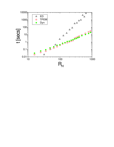
Figure 1: Computational time $t$ required to evaluate Eq. (5) in one Monte Carlo step per site as a function of the rank of the matrix $H$, $R_{H}$, using ED ($ZHEEV-LAPACK$ library, triangles), TPEM (squares) and Dyn (circles). Full parallelization capability was used for the TPEM and Dyn codes.

We can observe that for $R_{H}\gtrsim 64$, the present method and TPEM outperform the ED technique. For matrices smaller than 144x144, the TPEM technique is faster than Dyn, but this situation is reverted for matrices of size $R_{H}\geq 289$. This extraordinary performance can be understood intuitively by the following reasons: 1) The efficience of the recursive relation of the $\mid\nu_{k}\rangle$ vectors, 2) The functions $J_{k}\left(\tau\right)$ are relatively inexpensive to obtain computationallymotome , 3) No explicit multiplication between the $T_{k}(x)$ operators and the vectors $\mid i_{0}\rangle$ is necessary.noneed 4) The use of the parallelization capability. If only one CPU is used (no parallelization) in the Dyn (TPEM) algorithm, an increase in a factor of $R_{H}$ is obtained in the time consumption $t_{Dyn}$ ($t_{TPEM}$). In this case Dyn outperforms ED only for $R_{H}\gtrsim 900$.

V Case A: one orbital per site and FM configuration

The Dyn method can be directly tested with the analytical results for the density of states in cubic lattices for D=1, 2 and 3. This can be done by considering one orbital per site for Eq. (1), and the case where $\theta_{i}$ and $\varphi_{i}$ are constant for all $i$, that is the ferromagnetic (FM) phase where all the spins $\mathbf{{S}_{{i}}}$ are parallel. The effect of the phonons will not be considered and $H$ is normalized by the value $\mid\gamma_{\max}\mid=2Dt_{h}$.

The Dyn method basically is an efficient way to keep track of the time evolution of a wave-packet. In Fig. 2 can be seen the probability $\mid G(i_{0},j_{0};\tau)\mid^{2}$ as a function of the site $j_{0}$, when a particle is created at time $\tau=0$, in the 500$th$ site of a 1000-site chain and destroyed at a time $\tau$ later, considering periodic boundary conditions (PBC). In Fig. 2(a) the snapshot was taken at a time $\tau=1000$, where the wave-front is moving away from the $i_{0}$ site, indicated by the arrows. In the case 2(b) the wave-front has crossed the boundaries of the chain, and is moving towards the center of the chain, at a time $\tau=3600$.feiguin

It is possible to recover results for the infinite-size limit, provided the maximum time while the simulation $\tau_{sim}$ is carried out is less than the time that the ’wave front’ $\tau_{wf}$ reaches back to the site $i_{0}$, $\tau_{sim}<\tau_{wf}$. In the opposite limit, $\tau_{sim}\gg\tau_{wf}$, this method obtains the discrete resolution of the density of states spectra corresponding to a finite-lattice model.

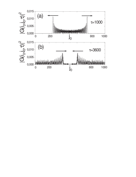
Figure 2: The probability $\mid G(i_{0},j_{0};\tau)\mid^{2}$ as a function of the site $j_{0}$, when a particle is created at time $\tau=0$, in the middle of a 1000-site chain (PBC), and measured at a time $\tau=1000$ later (a), and at a time $\tau=3000$ (b). The arrows show the direction of movement of the wave-front.

Figure 3: Time-dependence of $Im\left[G(i_{0},i_{0};\tau)\right]$ for the D=1 (black squares), D=2 (red circles) and D=3 (green triangles) cases, for lattice sites 1000, 100x100, and 50x50x50, respectively. The simulation is carried out up to the cut-off time $\tau_{sim}$. At time $\tau=0$, $Im\left[G(i_{0},i_{0};0)\right]$ =1, for D=1, 2 and 3.

Keeping track of the wave amplitude at the site $i_{0},$ will allow us to study the behavior of $G(i_{0},i_{0};\tau)$ for the different spatial dimensions. In Fig. 3 it is shown the time-dependence of $Im\left[G(i_{0},i_{0};\tau)\right]$ for the D=1 (black squares, 1000 sites), D=2 (red circles, 100x100 sites) and D=3 (green triangles, 50x50x50 sites) cases. The corresponding real component of $G(i_{0},i_{0};\tau)$ is zero.

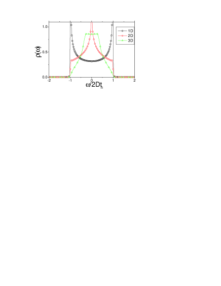
Figure 4: Frequency-dependence of $\rho\left(\omega\right)$ for the FM case in 1D (black squares), 2D (red circles) and 3D (green triangles).

After Fourier-transforming the value of $G(i_{0},i_{0};\tau)$, the corresponding densities of states $\rho\left(\omega\right)$ are obtained and shown in Fig. 4, and are in remarkably good agreement with analytical densities of states.Economou The simulations are carried out for the case $\tau_{sim}<\tau_{wf}$, where an approximation to $\rho\left(\omega\right)$ for an infinite system is obtained.

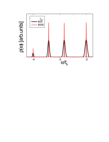
Figure 5: Electronic density $\rho\left(\omega\right)$ of states for a 8x8 cluster for the FM case in the energy interval [-4.25$t_{h}$,-1.75$t_{h}$], obtained using the Dyn method, with $\tau_{sim}$=800 (black line) and $\tau_{sim}$=8000 (red line). Details of the complete spectra found following the ED method are described in the text.

In order to compare the discrete nature of the density of states of finite clusters, a comparison of $\rho\left(\omega\right)$ for an 8x8 cluster of sites is given in Fig. 5, with $\tau_{sim}$=800 (black line), and $\tau_{sim}$=8000 (red line). The values picked for $\tau_{sim}$ correspond to the case $\tau_{sim}\gg\tau_{wf}$, and the greater the value of $\tau_{sim}$ the higher and narrower are the peaks obtained for $\rho\left(\omega\right)$, for that reason the distributions are not plotted on the same vertical scale. The distribution of eigenvalues obtained with ED is as follows (in units of $t_{h}$): $\pm$4, $\pm$3.41421, $\pm$2.82843, $\pm$2, $\pm$1.4142, $\pm$0.58579, and 0. The eigenvalues $\pm$4 are not degenerate, and the rest of them are four-fold degenerate with the exception of the eigenvalues $\pm$1.4142 (8 times), and the eigenvalue 0 (14 times). The peak positions obtained with Dyn are in good agreement with the ED results, where the precision is proportional to $\tau_{sim}$.

The finiteness of the time simulation $\tau_{sim}$ causes an oscillatory dependence in $\rho\left(\omega\right),$ and for values of $\omega$ close to the eigenvalues, $\rho\left(\omega\right)$ can have even small negative values. This behavior is commonly known as ’overshooting’ or Gibbs oscillations in the Fourier transformation context and these effects are treated here following the Kernel Polynomial approximationsilver . The peaks distributions obtained with $Dyn$ have a finite-frecuency width $\Delta\omega\approx\left(4D\pi\right)/\tau_{sim}$, where $4D$ is the electronic band-width in units of $t_{h}$.

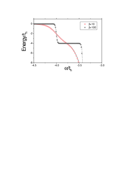
Figure 6: Electronic Energy vs. chemical potential. The full (red squares) and dashed lines (black triangles) correspond to the electronic energy obtained with the ED (Dyn) method at inverse temperatures $\beta$=10 and 100 respectively, for $\tau_{sim}$=400.

The total electronic energy is obtained by integration of $\rho\left(\omega\right),$ and in Fig. 6 its dependence vs. chemical potential $\mu$ is shown, where the full (red squares) and dashed lines (black triangles) corresponds to the electronic energy obtained with the ED ($Dyn$) method at inverse temperatures $\beta$=10 and 100 respectively, for $\tau_{sim}$=400. For the depicted $\omega-$range it can be observed at low temperatures two plateaus centered around the eigenvalues $-$4$t_{h}$ and $-$3,41421$t_{h}$, obtained after integrating the delta-shaped density of states.

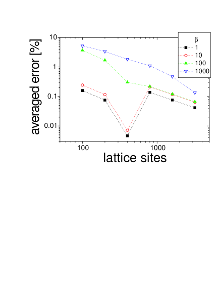
Figure 7: Averaged error of electronic energies as a function of $\tau_{sim}$, for values of $\beta$=1 (squares), 10 (circles), 100 (up triangles), and 1000 (down triangles).

We define the relative averaged error of the Dyn method in the electronic energy, for $\mu\in\left[-2Dt_{h},+2Dt_{h}\right]$ by,

$$\text{averaged error}=\frac{1}{N_{\tau_{sim}}}\sum_{i=1}^{N_{\tau_{sim}}}\frac{\sqrt{\left(E_{ED,i}-E_{Dyn,i}\right)^{2}}}{E_{ED,i}}$$

where the electronic energies $E_{ED,i}$ and $E_{Dyn,i}$ were calculated using both methods for $N_{\tau_{sim}}$=6400 equispaced frequencies in the interval $\left[-2Dt_{h},+2Dt_{h}\right]$, and plotted in Fig. 7 as a function of $\tau_{sim}$, for values of $\beta$=1 (squares), 10 (circles), 100 (up triangles), and 1000 (down triangles). We can observe that the averaged error is larger when $\beta$ increases, and decreases when $\tau_{sim}\,$is increased, but in a non-monotonic way, and it diverges for values of $\mu$ out of the band. In the present work, the $Dyn$ method will be used together with the MC technique for filling x=1/2, where the averaged error is less than 0.1%. High precision schemes can be achieved for the case when $\tau_{sim}/\tau_{wf}=L\gg 1$ and $L\lesssim mod(\tau_{sim},\tau_{wf})$, where $L$ is an integer number and $mod()$ is the modulus operation.

VI Case A: one orbital per site and PM configuration

The case of a random distribution for $\theta_{i}$ and $\varphi_{i}$: $\theta_{i}\in\left[0,\pi\right]$ and $\varphi_{i}\in\left[0,2\pi\right]$ is relevant in the present model of Eq. (1) as it represents a particular statistical realization of the paramagnetic (PM) phase, and it will be used as another test for the $Dyn$ method. In Fig. 8 it is shown the time dependence of $Im\left[G(i_{0},i_{0};\tau)\right]$ for the FM (full black line) and the PM (blue open circles) cases. In the last case, a random $i_{0}$ site in a D=2, $N$=6400 sites lattice (80x80) was chosen. We can see an irregular time dependence, with an average characteristic period longer than the FM case.

Figure 8: Time dependence of $Im\left[G(i_{0},i_{0};\tau)\right]$ for the FM (full black line) and the PM (blue open circles) cases, for a random-picked $i_{0}$ site in the 80x80 square lattice.

The corresponding PM local electronic density $\rho_{i_{0}}(\omega)$ is depicted in Fig. 9(a), for the same random-chosen site $i_{0}$. The total density of states can be obtained after averaging the local density of states $\rho(\omega)=\frac{1}{N}\sum_{i_{0}=1}^{N}\rho_{i_{0}}(\omega)$, for the particular random $\left\{\varphi_{i},\theta_{i}\right\}$ configuration considered (Fig. 9(b), red line). The disorder in the hopping distribution in the PM phase reduces the FM band-width (Fig. 9(b), black line) by a factor $1/\sqrt{2}$. The quantity $\rho(\omega)$ can be obtained analytically for the PM case after considering this reduction of the FM band-width, but the ED results are not shown here, since the CPU time needed is about 6 orders magnitude longer that the corresponding using the $Dyn$ method.

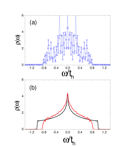
Figure 9: (a) Local density of states $\rho_{i_{0}}\left(\omega\right)$ for a random spin configuration $\left\{\varphi_{i},\theta_{i}\right\}$ on a 80x80 lattice. (b) Total density of states $\rho(\omega)=\frac{1}{N}\sum_{i_{0}=1}^{N}\rho_{i_{0}}(\omega)$ ($N$=6400) for the PM (red line) and the PM (black line) phases.

As the calculation of $\rho_{i_{0}}(\omega)$ is completely independent of the site considered, a speed-up of the algorithm should be achievable by means of a computational $parallel$ implementation.speedup

VII Case B: two orbitals per site and the MC algorithm for ground state

The full expression of Eq.(1) is taken into account, together with the consideration of two orbitals per site. The ground state is sampled through the calculation of the partition function, where the electronic component is given by:

$$\log Z_{el}=\int_{-\infty}^{+\infty}\rho\left(\omega\right)(1+e^{-\beta\left(\omega-\mu\right)})d\omega$$ (11)

obtained for each fixed proposed configuration the angles and displacements coordinates $\left\{\theta_{i},\varphi_{i},u_{x,i},u_{y,i},u_{z,i}\right\}$ for each site, and $\beta$ is the inverse temperature. The model is analyzed primarily using a classical Monte Carlo (MC) procedure for the localized spins and phonons, in conjunction with the ED and $Dyn$ methods for the electronic matrix. This last part of the process corresponds to the solution of the single-electron problem with hoppings determined by the localized spin and phonon configuration. The resulting electronic density is then filled with the number of electrons to be studied, that is, the simulations are carried out in the canonical ensemble.

A quantitative comparison of the electronic energies between both methods is given in Fig. 10, where the total averaged energies per site obtained using the ED (black triangles) and $Dyn$ (red circles) techniques, as a function of the parameter $J_{AF}/t$. The Monte Carlo simulations were performed on a 4x4 cluster, at a temperature $T/t$=0.025, $\lambda$=1.0, $\beta_{r}$=2 and filling $x$=1/2 (one particle every two sites). The vertical dashed lines represents approximately the values of $J_{AF}/t$ where the energy level crossings occur between the FM, the AF-type CE, and the AF-type G phases. The phase diagram for D=2 was already obtained using the ED method3 , and the Dyn method is in excellent quantitative agreement with these results.

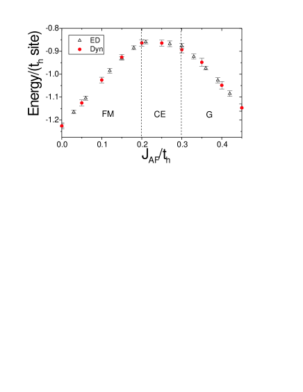
Figure 10: Total energies per site obtained for the effective manganites model (Eq. 1) using the ED (black triangles) and Dyn (red circles) techniques, as a function of the parameter $J_{AF}/t$. The Monte Carlo simulations were performed on a 4x4 cluster, at a temperature $T/t$=0.025, $\lambda$=1.0, $\beta_{r}=2$ and $x$=1/2. The dashed lines represents approximately the $J_{AF}/t$ where the energy level crossings occur between the FM, the AF-type CE, and the AF-type G phases.

VIII Results for D=3

Novel results for the phase diagram x=1/2, $\lambda$=0.5, D=3 at $T/t_{h}$=0.02 were obtained following MC+Dyn simulations on a 12x12x12 cluster (3456 orbitals). The maximum number of momenta considered was $K_{max}$=100 or 200, and the number of Monte Carlo steps per site (MCS/S) was typically taken as 5000. Full parallelization of the algorithm was performed, where tipically 288 cpus where dedicated to compute a single task. Updates of the spin and phononic $\left\{\theta_{i},\varphi_{i},u_{x,i},u_{y,i},u_{z,i}\right\}$ configurations were accepted or rejected according to the Metropolis algorithm. The simulations start in most of the cases with random initial configurations, but for the A and CE phases the convergence is very slow, specially close to the energy crossovers. A speed up of the convergence was realized by fixing the corresponding spin configurations, and testing the stability of the proposed ground state as a function of MCS/S. The magnetic character of the different ground states were analyzed by means of Spin Structure Factor $S(\mathbf{{q})=}1/N^{\mathbf{2}}\mathbf{\sum_{i,j}\langle{S}_{i}{.S}_{j}\rangle e^{i\mathbf{q}{.}({r}_{i}-{r}_{j})}}$. For the 12x12x12 cluster, the $\mathbf{q}$ values considered are: ($l\pi/6$,$k\pi/6$,$m\pi/6$), where $l$, $k$ and $m$ are integers values in the interval $0\leq l,k,m\leq 6.$

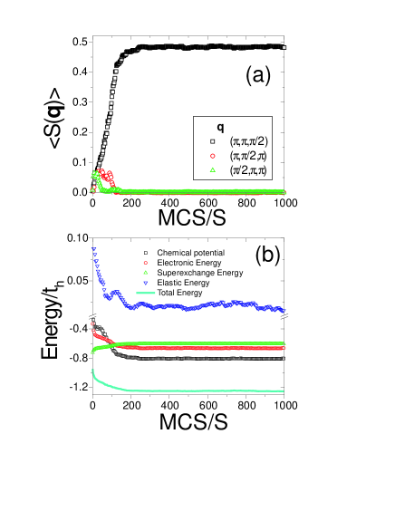
Figure 11: (a) $S(\mathbf{{q})}$ vs. MCS/S for $J_{AF}/t_{h}$=0.3, x=1/2, $\lambda$=0.5, D=3 at $T/t_{h}$=0.02 on a 12x12x12 cluster and $\mathbf{q}=(\pi,\pi,\pi/2)$ (black squares), $\mathbf{q}=(\pi,\pi/2,\pi)$ (red circles) and $\mathbf{q}=(\pi/2,\pi,\pi)$ (green triangles). The ground state corresponding to this setup of parameters is the dimer phase. (b) Chemical potential $\mu$ (black squares), electronic (red circles), superexchange (green up triangles), elastic (blue down triangles) and total energies (cyan line) vs. MCS/S.

In Fig. 11(a) it is shown $S(\mathbf{{q})}$ vs. MCS/S for $J_{AF}/t_{h}$=0.3 and $\mathbf{q}=(\pi,\pi,\pi/2)$ (black squares), $\mathbf{q}=(\pi,\pi/2,\pi)$ (red circles) and $\mathbf{q}=(\pi/2,\pi,\pi)$ (green triangles). The ground state corresponding to this setup of parameters is the dimer phase, which consists of pairs spins $\uparrow\uparrow,$ aligned antiferromagnetically between them. This phase is evidenced by a single peak $S(\mathbf{{q})=}1/2$ at one of these $\mathbf{q}$ values chosen. For MCS/S$\lesssim$150 the dimer correlations between neighboring spins are pointing in all the three spatial directions. For MCS/S$>$200, the system breaks the spatial isotropy, and all the cluster consist of dimers aligned in the $z$-direction, for this particular example, and for MCS/S$>$400 the system has reached thermal equilibrium. In Fig. 11(b) it is shown the Chemical potential $\mu$ (black squares), electronic (red circles), superexchange (green up triangles), elastic (blue down triangles) and total energies (cyan line) vs. MCS/S. The Chemical potential $\mu$ is calculated autoconsistently at each Monte Carlo step to fix the electronic density to $x=0.5\pm 0.00001$. The electronic energy is given by the first and fourth terms in Eq. (1), the superexchange energy involves the second term and the elastic energy is given by the fifth term.

The total energies per site of the ground states are plotted as a function of the parameter $J_{AF}/t_{h}$ in Fig. 12, under the same conditions used in Figs. 11. As the $J_{AF}/t_{h}$ parameter is increased, the AF-insulating character of the ground states obtained increases. Comparing this picture with the phase diagrams for D=2 (Fig. 10), we notice the appearance of the A and dimer phases for the case D=3. The A-phase, which consists of FM planes aligned antiferromagnetically between them, and the FM-phase are degenerate for D=2, but for the case D=3 their corresponding total energies are different, i.e. the degeneracy is removed. The dimer phase, which was obtained in D=1 and 24 considering one orbital per site, is not a ground state in D=2 with two orbitals per site due to the explicitly breaking of the symmetry between $d_{x^{2}-y^{2}}\$and $d_{3z^{2}-r^{2}}$ orbitals.

Increasing the insulating parameter $J_{AF}/t_{h}$ the following sequence of phases is obtained: FM, A, CE, dimer and G. It is worth to note that, with the exception of the dimer phase, these phases have been observed experimentally in half-doped manganites,tomioka ; kuwahara ; okimoto ; wollan ; jirac following approximately the same sequence.kajimoto

For values of $J_{AF}/t_{h}$ in the interval $\left[0,0.125\right]$ the ground state of the system corresponds to the metallic FM phase. The orbital configuration of this phase is highly degenerate, but analyzing snapshots at finite temperature orbital states of the form cos$\left(\Theta\right)\mid d_{x^{2}-y^{2}}\rangle+$sin$\left(\Theta\right)\mid d_{3z^{2}-r^{2}}\rangle$ with random values of $\Theta$ in the range $0\leq\Theta\leq 2\pi$ are observed, namely the orbital state of this phase is completely disordered with an homogeneous distribution of the charges.

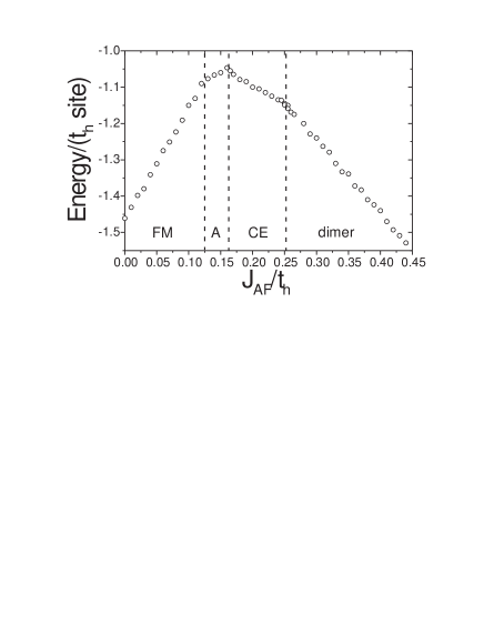
Figure 12: Total energies per site of the ground states as a function of the parameter $J_{AF}/t_{h}$ for the same conditions as in Fig. 11.

The A-phase is found for values of $J_{AF}/t_{h}$ in the interval $\left[0.125,0.16\right]$. The orbital distribution corresponds to a majority occupation of the planar $d_{x^{2}-y^{2}}$ orbitals, which favors a metallic in-plane conductivity. At the same time this orbital arrangement favors the AF alignment between neighboring FM planes, where the hopping process inter-planes is strongly suppressed. This phase has been observed in the Pr_0.5Sr_0.5MnO₃tomioka and Nd_0.5Sr_0.5MnO₃kuwahara compounds, in this last case in coexistence with the CE-phase.

For values of $J_{AF}/t_{h}$ in the approximate interval $\left[0.16,0.26\right]$ the ground state of the system corresponds to the CE-phase.okimoto This magnetic phase was measured experimentally in the systems La_0.5Ca_0.5MnO₃wollan , Nd_0.5Sr_0.5MnO₃kuwahara , and Pr_0.5Ca_0.5MnO₃jirac . Even for $\lambda$=0, the character of this phase is insulating and was analyzed in several theoretical workshottaCE ; vbrink ; 3 , were the details of the spin, charge and orbital configuration can be seen.commentI

The dimer phase, which is the ground state of the model in $J_{AF}/t_{h}\in\left[026,0.66\right]$ for D=3, was also obtained in D=1 and 24 . The existence of FM dimers (Zener Polarons) along the zigzag chains of the CE-phase has being observed in Pr_0.6Ca_0.4MnO₃aladine compounds, together with a dimerization of the Mn-Mn distances. More complex interactions should be included in the present model, like the displacement of the Mn cations together with the distance dependence of the couplings $J_{AF}$ and $t_{h}$ in oder to reproduce this phase. For the pairs $\uparrow\uparrow$ directed in the $\xi=\mathbf{x},$ $\mathbf{y}$ or $\mathbf{z}$ spatial directions, the orbital configuration of the dimers phase corresponds to orbitals $d_{3\xi^{2}-r^{2}}.$

Finally, for values $J_{AF}/t_{h}\gtrsim 0.66$ the insulating $G$ phase is obtained. The range of parameters where the G and dimer phases are present corresponds to manganites with very small band-width and sofar has not been experimentally observed up to date.

IX Conclusions

In this work it was described an efficient high-performance algorithm to calculate the local time-dependent Green’s operator for general hermitian, time-independent, linear differential operator $H$, expressed in matrix form. The time-dependent local Green’s operator is expressed as a finite series of the Chebyshev polynomials of the normalized $H$ operator, multiplied by the corresponding Bessel function of the first kind5 . This approach, together with the fact that in the local basis no multiplication of matrices by vectors is needed to keep track of the time-evolution of an initial state, leads to an algorithm where CPU time and memory scale linearly with the number of states in the basis of the Hilbert space.

The total energies of an effective Hamiltonian for manganites were compared using the Exact Diagonalization technique and the novel Dyn method. The results obtained with both ED and Dyn methods were in general good agreement, and for lattices larger than 289 sites the Dyn method outperforms the ED and TPEM techniques. A parallelization of the algorithm is possible, with a speed-up factor close to the number of processors involved. The Dyn method could become the method of choice to expand the present computational limitations set by the ED method, and in particular to study the model for D=3.

It was shown that it is possible to recover results for the infinite-size limitfeiguin , provided the maximum time of the simulation on a finite-lattice is less than the time that the ’wave front’ reaches back to the site $i_{0}$, $\tau<\tau_{sim}$. The discreteness nature of the spectra is obtained in the opposite limit, $\tau\gg\tau_{sim}$.

The Dyn method used together with the Monte Carlo technique was used to obtain new results for the manganites phase diagram for D=3 and half-filling in a 12x12x12 cluster (3456 orbitals). As a function of an insulating parameter we found the following sequence of ground states: FM, AF-type A, AF-type CE, dimer and AF-type G. These phases are in remarkable agreement with experimental results in half-doped manganites,tomioka ; kuwahara ; okimoto ; wollan ; jirac which follow approximately the same sequence.kajimoto

X Acknowledgements

We are grateful to A. A. Aligia, M. Kollar, D. Vollhardt, and V. V. Dobrovitski for helpful discussions and to G. Alvarez for providing the TPEM code. The CSIT at FSU and the Forschungszentrum at Juelich are also acknowledged. This work was supported by the Deutsche Forschungsgemeinschaft through SFB 484 (BN).

References

- (1) T. A. Kaplan and S. D. Mahanti, editors, Physics of Manganites, Kluwer Academic/Plenum Publishers, New York, 1998; Y. Tokura, editor, Colossal Magnetoresistive Oxides, Gordon and Breach, 2000; E. Dagotto, Nanoscale Phase Separation and Colossal Magnetoresistance, Springer-Verlag, Berlin, 2002.
- (2) Y. Motome, N. Furukawa, and N. Nagaosa, Phys. Rev. Lett. 91, 167204 (2003). S. Yunoki, A. Moreo, and E. Dagotto, Phys. Rev. Lett. 81, 5612 (1998).
- (3) E. Dagotto, S. Yunoki, A. L. Malvezzi, A. Moreo, J. Hu, S. Capponi, D. Poilblanc, and N. Furukawa, Phys. Rev. B 58, 6414 (1998).
- (4) H. Aliaga, D. Magnoux, A. Moreo, D. Poilblanc, S. Yunoki, and E. Dagotto, Phys. Rev. B 68, 104405 (2003).
- (5) T. Hotta, M. Moraghebi, A. Feiguin, A. Moreo, S. Yunoki, and E. Dagotto. Phys. Rev. Lett. 90, 247203 (2003). H. Aliaga, B. Normand, K. Hallberg, M. Avignon, and B. Alascio. Phys. Rev. B 64, 024422 (2001). D. J. Garcia, K. Hallberg, C. D. Batista, S. Capponi, D. Poilblanc, M. Avignon, and B. Alascio. Phys. Rev. B 65, 134444 (2002).
- (6) Y. Motome and N. Furukawa, J. Phys. Soc. Jpn. 68, 3835 (1999). Y. Motome and N. Furukawa, J. Phys. Soc. Jpn. 72, 2126 (2003). N. Furukawa and Y. Motome, J. Phys. Soc. Jpn. 73 No.6 (2004) 1482-1489.
- (7) V. V. Dobrovitski, H. A. De Raedt, M. I. Katsnelson, and B. N. Harmon. Phys. Rev. Lett. 90, 210401 (2003). V. V. Dobrovitski and H. A. De Raedt. Phys. Rev. E 67, 056702 (2003). J. S. Kole, M. T. Figge, and H. De Raedt. Phys. Rev. E 64, 066705 (2001).
- (8) M. N. Iliev, M. V. Abrashev, H.-G. Lee, V. N. Popov, Y. Y. Sun, C. Thomsen, R. L. Meng, and C. W. Chu, Phys. Rev. B 57, 2872 (1998); T. Hotta, S. Yunoki, M. Mayr, and E. Dagotto, Phys. Rev. B 60, R15009-R15012 (1999).
- (9) E. N. Economou, Green’s functions in quantum physics. Springer-Verlag, 1983.
- (10) That means that we can pick arbitrarily large values for , but at the same time we will need to calculate longer time evolutions.
- (11) The numerical accuracy of the computer-generated Bessel function of the first kind is reduced substantially for arguments greater than 75. In order to avoid this problem, the initial state have to be refreshed periodically, for times 75.
- (12) The TPEM techniquemotome1 is based on the expansion of in terms of Chebyshev polynomials: . The momenta are calculated after numerical integration of: at each Monte Carlo step and value of , while for Dyn case the equivalent momenta are just plain machine functions. The TPEM code used in this work was provided by G. Alvarez.
- (13) It is worthy to remark, that despite the matricial nature of the operators in the series expansion given by Eq.(9), no matrices or multiplication of matrices and vectors are needed in the code of the algorithm. For a more specific example, let’s assume we have free spin-less fermions in a chain of three sites, and (the parameter is already normalized) and we want to trace the evolution of the initial state . Following Eq.(9), we obtain: , , , and so on.
- (14) S. R. White and A. Feiguin, preprint: cond-mat/0403310.
- (15) R. N. Silver, H. Roeder, A. F. Voter, and D. J. Kress, J. of Comp. Phys. 124, 115 (1996). A. Weisse, Eur. Phys. J. B 40, 125 (2004).
- (16) The speed-up factor in this case is close to the number of procesors, . Each of the processor must evaluate the described algorithm starting with a different initial state , and then they must communicate only the fourier-transformed value of to a single processor, which it in turn performs the summation.
- (17) Y. Tomioka, A. Asamitsu, Y. Moritomo, H. Kuwahara, and Y. Tokura, Phys. Rev. Lett. 74, 5108 (1995).
- (18) H. Kuwahara, T. Okuda, Y. Tomioka, A. Asamitsu, and Y. Tokura, Phys. Rev. Lett. 82, 4316 (1999).
- (19) P. Radaelli et al., Phys. Rev. B 59, 14440 (1999). Y. Okimoto et al., Phys. Rev. Lett. 75, 109 (1995).
- (20) E. D. Wollan and W. C. Koehler, Phys. Rev. 100, 545 (1955).
- (21) Z. Jirac, S. Krupicka, Z. Simsa, M. Dlouha, and S. Vratislav, J. Mag. Mag. Mat. 53, 153 (1985).
- (22) R. Kajimoto, H. Yoshizawa, Y. Tomioka, and Y. Tokura, Phys. Rev. B 66, 180402(R) (2002). C. Autret, Ph.D. Thesis, 2002 Universite de Caen.
- (23) T. Hotta, Y. Takada, H. Koizumi, and E. Dagotto, Phys. Rev. Lett. 84, 2477 (2000).
- (24) J. van den Brink, G. Khaliullin, and D. Khomskii, Phys. Rev. Lett. 83, 24 (1999).
- (25) The and phasesvbrink have not being observed as ground states of the present model in 3D, with the exemption of 4x4x4 clusters and for fillings 0.45. However it is remarkable that the energies per site of the phases and are normally as close as 0.02in clusters 4x4x4, 8x8x8 and 12x12x12.
- (26) A. Daoud-Aladine, J. Rodríguez-Carvajal, L. Pinsard-Gaudart, M. T. Fernández-Díaz, and A. Revcolevschi, Phys. Rev. Lett. 89, 129902(E) (2002)