The Strong Coupling Fixed-Point Revisited

Abstract

In recent work we have shown that the Fermi liquid aspects of the strong coupling fixed point of the s-d and Anderson models can brought out more clearly by interpreting the fixed point as a renormalized Anderson model, characterized by a renormalized level $\tilde{\epsilon}_{d}$, resonance width, $\tilde{\Delta}$, and interaction $\tilde{U}$, and a simple prescription for their calculation was given using the numerical renormalization group (NRG). These three parameters completely specify a renormalized perturbation theory (RPT) which leads to exact expressions for the low temperature behaviour. Using a combination of the two techniques, NRG to determine $\tilde{\epsilon}_{d}$, $\tilde{\Delta}$, and $\tilde{U}$, and then substituting these in the RPT expressions gives a very efficient and accurate way of calculating the low temperature behaviour of the impurity as it avoids the necessity of subtracting out the conduction electron component. Here we extend this approach to an Anderson model in a magnetic field, so that $\tilde{\epsilon}_{d}$, $\tilde{\Delta}$, and $\tilde{U}$ become dependent on the magnetic field. The de-renormalization of the renormalized quasiparticles can then be followed as the magnetic field strength is increased. Using these running coupling constants in a RPT calculation we derive an expression for the low temperature conductivity for arbitrary magnetic field strength.

1 Introduction

After Wilson’s seminal numerical renormalization group (NRG) solution of the spin 1/2 s-d model [1] it was very soon recognized by Nozières [2] that the low energy strong coupling fixed point corresponds to Fermi liquid behaviour. Using a phenomenological description of the phase shift Nozières then gave an analytic derivation of Wilson’s result for the ”$\chi/\gamma$” ratio $R$[3], $R=2$, and derived the leading form of the low temperature conductivity in terms of the Kondo temperature [2]. The important characteristic of a Fermi liquid is the 1-1 correspondence of the single particle excitations with those of the non-interacting system. This correspondence does not apply in the case of the s-d model because the model has a constraint of a fixed occupancy $n_{d}$ of the impurity site, $n_{d}=1$ for $S=1/2$, which implies a strong local interaction to enforce it. The Anderson model, however, which is equivalent to the s-d model ($S=1/2$) in the local moment regime, is truly non-interacting when the interaction term $U$ is set to zero, so the 1-1 correspondence of the single particle excitations with those of the non-interacting system should hold, even in the local moment limit. This implies that low energy fixed point of the s-d model and Anderson model should be described more naturally in terms of a renormalized Anderson model. The Anderson model [4] has the form,

$$H_{\rm AM}=\sum_{\sigma}\epsilon_{d}d^{\dagger}_{\sigma}d_{\sigma}+Un_{d,\uparrow}n_{d,\downarrow}+\sum_{{k},\sigma}(V_{k}d^{\dagger}_{\sigma}c_{{k},\sigma}+V_{k}^{*}c^{\dagger}_{{k},\sigma}d_{\sigma})+\sum_{{k},\sigma}\epsilon_{{k},\sigma}c^{\dagger}_{{k},\sigma}c_{{k},\sigma},$$ (1)

where $\epsilon_{d}$ is the energy of the impurity level, $U$ the interaction at the impurity site, and $V_{k}$ the hybridization matrix element to a band of conduction electrons with energy $\epsilon_{k}$.When $U=0$ the local level broadens into a resonance, corresponding to a localized quasi-bound state, whose width depends on the quantity $\Delta(\omega)=\pi\sum_{k}|V_{k}|^{2}\delta(\omega-\epsilon_{k})$. It is usual to consider the case of a wide conduction band with a flat density of states where $\Delta(\omega)$ becomes independent of $\omega$ and can be taken as a constant $\Delta$.

In the wide conduction band limit the one-electron Green’s function, $G_{d}(\omega)$ takes the form

$$G_{d}(\omega)={1\over\omega-\epsilon_{d}+i\Delta-\Sigma(\omega)}$$ (2)

where $\Sigma(\omega)$ is the self-energy and $\Delta$ is the width of the resonance at $\epsilon_{d}$ when $U=0$. Near the Fermi level for small $\omega$, $\Sigma(\omega)=\Sigma(0)+\omega\Sigma^{\prime}(0)+{\rm O}(\omega^{2})$, and if this is substituted into (2) then for small $\omega$ the denominator is of the same form as that for the non-interacting system with a renormalized level $\tilde{\epsilon}_{d}$ and resonance width $\tilde{\Delta}$ given by

$$\tilde{\epsilon}_{\rm d}=z(\epsilon_{\rm d}+\Sigma(0)),\quad\tilde{\Delta}=z\Delta,$$ (3)

where $z$, the wavefunction renormalization factor, is given by $z={1/{(1-\Sigma^{\prime}(0))}}$, and the prime indicates a derivative with respect to $\omega$. The 1-1 correspondence is evident when one calculates the quasiparticle occupation number $\tilde{n}_{d}$ at $T=0$,

$$\tilde{n}_{d\sigma}={1\over 2}-{1\over\pi}\tan^{-1}\left({\tilde{\epsilon}_{{\rm d}}}\over{\tilde{\Delta}}\right)=n_{d\sigma},$$ (4)

which is equal to the impurity occupation number $n_{d\sigma}$ for spin $\sigma$ at $T=0$ from the Friedel sum rule [5]. The corresponding quasiparticle density of states $\tilde{\rho}_{d}(\omega)$ is given by

$$\tilde{\rho}_{d}(\omega)={\tilde{\Delta}/\pi\over(\omega-\tilde{\epsilon}_{d})^{2}+\tilde{\Delta}^{2}}.$$ (5)

It follows from Fermi liquid theory that the impurity specific heat coefficient $\gamma$, as calculated from these non-interacting quasiparticles, is exact as $T\to 0$, and is given by

$$\gamma_{\rm imp}={2\pi^{2}\over 3}\tilde{\rho}_{d}(0).$$ (6)

In the original NRG calculations for the Anderson model the low energy fixed point was analysed as a strong coupling $V\to\infty$ fixed point [6]. In this limit the impurity is decoupled, and so the analysis does not bring out the 1-1 correspondence of the single particle excitations with those of the original Anderson model. Recently we (Hewson, Oguri and Meyer[7]) have reanalysed the strong coupling fixed point as a $U=0$ fixed point with a finite $V$, which leads directly to the renormalized parameters $\tilde{\epsilon}_{d}$ and $\tilde{\Delta}$. The NRG calculations are based on linear chain form for the Anderson model, with a discretized conduction electron spectrum and a discretization parameter $\Lambda>1$. Starting with the impurity at the end of the chain, the Hamiltonians corresponding to a finite lengths of chain are diagonalized iteratively, adding a new site to the chain with each iteration. If the lowest energy single-particle $E_{p}(N)$ or single-hole excitations $E_{h}(N)$ of the interacting Anderson model for a chain with $N+2$ sites can be described by a non-interacting renormalized Anderson model then $E=E_{p}(N)$ or $E=E_{h}(N)$ should satisfy the equation,

$${E\Lambda^{-(N-1)/2}}-\tilde{\epsilon}_{d}(N)=\Lambda^{(N-1)/2}\tilde{V}(N)^{2}g_{00}(E),$$ (7)

where the effective parameters, $\tilde{\epsilon}_{d}(N)$ and $\tilde{\Delta}(N)=\pi\tilde{V}(N)^{2}/D$, should be independent of $N$. The function $g_{00}(\omega)$ is the local Green’s function for the first conduction electron site of the chain when decoupled from the impurity ($V=0$) (see [7] for details).

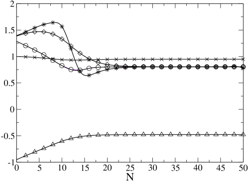
Figure 1: Plots of the parameters, $\tilde{\Delta}(N)/\Delta$ (crosses), $\tilde{\epsilon}_{d}(N)/\pi\Delta$ (triangles), $\tilde{U}_{pp}(N))/\pi\Delta$ (diamonds), $\tilde{U}_{hh}(N)/\pi\Delta$ (stars) and $\tilde{U}_{ph}(N)/\pi\Delta$ (circles), with $N$, for the Anderson model with bare parameters, $U=0.04$, $\pi\Delta=0.03$, and $\epsilon_{d}=-0.05$. In this and subsequent figures the full lines are interpolations using the calculated data points.

In Figs. 1 and 2 we present results for $\tilde{\epsilon}_{d}(N)$ and $\tilde{\Delta}(N)$, determined by these two equations as a function of $N$. In the first case shown in figure 1 we take a relatively weak coupling example with bare parameters, $\pi\Delta=0.03$, $\epsilon_{d}=-0.05$ and $U=0.04$ (bandwidth $2D=2$ in all cases), which is such that $U\rho_{d,{\rm mf}}(0)=0.331<1$, where $\tilde{\rho}_{d,{\rm mf}}(0)$ is the mean field density of states at the Fermi level, $\tilde{\rho}_{d,{\rm mf}}(0)=\Delta/\pi(\tilde{\epsilon}_{d,{\rm mf}}^{2}+\Delta^{2})$ with $\tilde{\epsilon}_{d,{\rm mf}}=\epsilon_{d}+Un_{d,{\rm mf}}/2$, and so does not satisfy the mean field (Hartree-Fock) criterion for a local moment. The renormalized parameters are independent of $N$ for $N>26$, which confirms that these single-particle excitations on the lowest energy scale can indeed be described by a renormalized Anderson model. The asymptotic value of $\tilde{\Delta}/\Delta=0.947$ for large $N$, and so $\tilde{\Delta}$ differs little from its bare value. The value of $\tilde{\epsilon}_{d}=-0.0143$, and is very approximately of the same order as that predicted from mean field theory $\tilde{\epsilon}_{d,{\rm mf}}=-0.0166$.

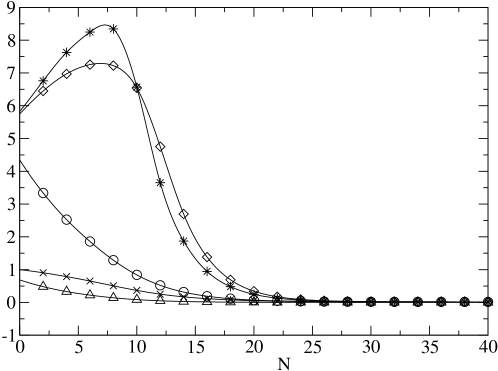
Figure 2: Plots of the parameters, $\tilde{\Delta}(N)/\Delta$ (crosses), $\tilde{\epsilon}_{d}(N)/\pi\Delta$ (triangles), $\tilde{U}_{pp}(N))/\pi\Delta$ (diamonds), $\tilde{U}_{hh}(N)/\pi\Delta$ (stars) and $\tilde{U}_{ph}(N)/\pi\Delta$ (circles), with the $N$, for the Anderson model with bare parameters, $U/\pi\Delta=5.0$, $\pi\Delta=0.03$, and $\epsilon_{d}=-0.05$ .

In Fig. 2 we give the corresponding results for $U=0.15$, keeping the other parameters the same. For this value of $U$ mean field theory would predict the breaking of local spin symmetry as $U\tilde{\rho}_{d,{\rm mf}}(0)=2.02>1$, and hence this case corresponds to a system with a local moment and can be described by an effective s-d model. We see a considerable renormalization such that $\tilde{\Delta}/\Delta=0.0158$, and $\tilde{\epsilon}_{d}$ becomes very small $\tilde{\epsilon}_{d}=1.06\times 10^{-5}$ so the effective level is very close to the Fermi level, as to be expected in the almost localized limit $n_{d}\approx 1$. Having determined $\tilde{\epsilon}_{d}$ and $\tilde{\Delta}$, the impurity occupation and the specific heat coefficient $\gamma$ can be determined from eqs. (4) and (6).

The renormalized quasiparticles must interact with one another, and this interaction must come into play as soon as two or more single particle excitations are created from the interacting ground state. If the lowest two-particle excitation from the ground state for the interacting system for a given $N$ has an energy $E_{pp}(N)$, then we can calculate $\tilde{U}$ by equating the energy difference $E_{pp}(N)-2E_{p}(N)$ to that calculated by adding an local interaction term to the effective Anderson model for the non-interacting quasiparticles[6, 7]. For finite $N$ we can use this equation to define an $N$-dependent renormalized interaction $\tilde{U}_{pp}(N)$,

$$E_{pp}(N)-2E_{p}(N)=\tilde{U}(N)\Lambda^{(N-1)/2}|\psi_{p,1}^{*}(-1)|^{2}|\psi_{p,1}^{*}(-1)|^{2},$$ (8)

where $|\psi_{p,1}(-1)|^{2}$ is given by

$$|\psi_{p,1}|^{2}={1\over 1-\tilde{V}^{2}(N)\Lambda^{(N-1)}{g^{\prime}}_{00}(E_{p}(N))},$$ (9)

where ${g^{\prime}}_{00}(\omega)$ is the derivative of $g_{00}(\omega)$.

Alternatively we could consider the same procedure for a two hole excitation $E_{hh}(N)$ and in a similar way define an $N$-dependent renormalized interaction $\tilde{U}_{hh}(N)$, or a particle-hole excitation $E_{ph}(N)$ to define a renormalized interaction $\tilde{U}_{ph}(N)$. In this latter case, as a positive $U$ leads to particle-hole attraction, we use $E_{p}(N)+E_{h}(N)-E_{ph}(N)$ on the left-hand side of eq. (8).

If these two particle excitations can be described by an effective Anderson model then $\tilde{U}_{pp}(N)$, $\tilde{U}_{hh}(N)$ and $\tilde{U}_{ph}(N)$ should be independent of $N$ and also independent of the particle and hole labels. The values of $\tilde{U}_{pp}(N)$, $\tilde{U}_{hh}(N)$ and $\tilde{U}_{ph}(N)$, for the case $U=0.04$ as a function of $N$ are shown in Fig. 1, and those for $U=0.15$ in Fig. 2, where $\pi\Delta=0.03$ and $\epsilon_{d}=-0.04$ in both cases. The three interaction parameters can be seen to converge to a unique value for large $N$ both in the weak and strong coupling cases.

In Fig. 3 the renormalized interaction parameters in the strong coupling case for $N>25$ of the plot given in Fig. 2 are shown over a smaller energy range. It can be seen that $\tilde{U}_{pp}(N)$, $\tilde{U}_{hh}(N)$ and $\tilde{U}_{ph}(N)$ not only have a unique limit but that this limit coincides with the asymptotic value of $\pi\tilde{\Delta}(N)$ for large $N$, so that $\pi\tilde{\Delta}=\tilde{U}$; consequently there is only one effective parameter scale in the localized (Kondo) regime.

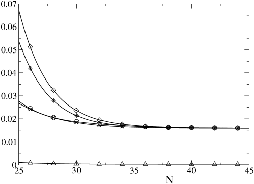
Figure 3: The same plot as in Fig. 2 for $N>25$ but shown over a smaller energy range. The parameters correspond to the almost localized (Kondo) limit; the renormalized level $\tilde{\epsilon}_{d}/\pi\Delta$ (triangles) is very close to the Fermi level, and the limiting value of $\tilde{\Delta}(N)/\Delta$ for large $N$ (crosses) coincides with the limiting values of $\tilde{U}_{pp}(N))/\pi\Delta$ (diamonds), $\tilde{U}_{hh}(N)/\pi\Delta$ and $\tilde{U}_{ph}(N)/\pi\Delta$ (circles).

2 Renormalized Perturbation Theory

An alternative renormalization approach to the Wilson technique is the renormalized perturbation theory (RPT)[8] as originally developed to deal with the infinities arising in quantum electrodynamics (QED). While the Wilson approach is based on the progressive elimination the higher order excitations to obtain an effective low energy model, the renormalized perturbation theory is essentially a reorganization of perturbation theory so that a perturbation expansion can be carried for the same model, but in terms of parameters appropriately renormalized for very low energy scales. These low energy scales are where almost all observations are made in QED so that the renormalized parameters can be taken from experiment. As the RPT is not simply about the cancellation of infinities, but working with parameters appropriate to the energy scale under investigation, it can be applied quite generally. This approach has been developed for the Anderson model, and leads naturally to the quasiparticle description[9, 10]. Here we briefly review some of the main results which will be required in the later sections of this paper. The renormalized parameters of the non-interacting quasiparticles are a renormalized level $\tilde{\epsilon}_{d}$ and resonance width $\tilde{\Delta}$, as given in eq. (3) in terms of the self-energy and its derivative at $T=\omega=0$. The renormalized local interaction $\tilde{U}$ is identified with the fully dressed irreducible 4-vertex, $\Gamma_{\uparrow\downarrow}(\omega_{1},\omega_{2},\omega_{3},\omega_{4})$ at $\omega_{1}=\omega_{2}=\omega_{3}=\omega_{4}=0$,

$$\tilde{U}=z^{2}\Gamma_{\uparrow\downarrow}(0,0,0,0),$$ (10)

which is rescaled by $z^{2}$ so the propagator for the quasiparticles is normalized.

In applying the renormalized perturbation expansion the Lagrangian for the Anderson model ${\cal L}_{\rm AM}(\epsilon_{d},\Delta,U)$ is rewritten in the form,

$${\cal L}_{\rm AM}(\epsilon_{d},\Delta,U)={\cal L}_{\rm AM}(\tilde{\epsilon}_{d},\tilde{\Delta},\tilde{U})+{\cal L}_{\rm c}(\lambda_{1},\lambda_{2},\lambda_{3}).$$ (11)

The first term on the right hand side is simply the Lagrangian for the Anderson model expressed in terms of the renormalized parameters, and the second part is the remainder or counter term. The three parameters $\lambda_{1}$, $\lambda_{2}$ and $\lambda_{3}$ are fully determined order by order in the expansion in powers of $\tilde{U}$ by the requirement that they prevent overcounting and cancel off any terms that further renormalize the particles as these quantities have be taken to be fully renormalized already. Hence the three renormalized parameters $\tilde{\epsilon}_{d}$, $\tilde{\Delta}$ and $\tilde{U}$ are sufficient to specify the RPT precisely.

The first order perturbation theory in $\tilde{U}$ gives results for the impurity spin and charge susceptibilities at $T=0$,

$$\chi_{s}={(g\mu_{\rm B})^{2}\over 2}\tilde{\rho}_{d}(0)(1+\tilde{U}\tilde{\rho}_{d}(0)),\quad\chi_{c}=2\tilde{\rho}_{d}(0)(1-\tilde{U}\tilde{\rho}_{d}(0)),$$ (12)

where $\tilde{\rho}_{d}(\omega)$ is given by eq. (5). These results can shown to be exact by the use of a Ward identity, and are equivalent to the results as first derived by Yamada[12] from an analysis of a perturbation expansion in powers of $U$. The ‘$\chi/\gamma$’ ratio $R$ is then given by $R=1+\tilde{U}\tilde{\rho}_{d}(0)$.

The RPT result for the renormalized self-energy to second order in $\tilde{U}$ for the symmetric model gives the exact low temperature result for the conductivity $\sigma(T)$ to second order in the temperature $T$, which is given by

$$\sigma(T)=\sigma_{0}\left\{1+{\pi^{2}\over 3}\left(T\over\tilde{\Delta}\right)^{2}\left[1+2\left({\tilde{U}\over\pi\tilde{\Delta}}\right)^{2}\right]+{\rm O}(T^{4})\right\}.$$ (13)

When the renormalized parameters are expressed in terms of the self-energy and the vertex function these results coincide with the exact expressions derived by Yamada and Yosida [12] from an analysis of perturbation theory to all orders $U$, and in the localized regime ($\tilde{U}/\pi\tilde{\Delta}\to 1$) with the Fermi-liquid results of Nozières [2]. The corresponding result for the differential conductance through a quantum dot to second order in the applied voltage has been given by Oguri[13].

Higher order terms in $\tilde{U}$ can be used to estimate the leading corrections to the Fermi liquid results[10]. Estimates of the induced magnetization $M(h)$ as a function of magnetic field $H$, where $h=g\mu_{\rm B}H/2$ to order $H^{3}$ have been made using RPT to third order in $\tilde{U}$ for the particle-hole symmetric model. The result to this order is

$$M(h)={g\mu_{\rm B}\over\pi}\left\{\left(1+{\tilde{U}\over\pi\tilde{\Delta}}\right)\left({h\over\tilde{\Delta}}\right)+\left[1+4\left({\tilde{U}\over\pi\tilde{\Delta}}\right)+A\left({\tilde{U}\over\pi\tilde{\Delta}}\right)^{2}+B\left({\tilde{U}\over\pi\tilde{\Delta}}\right)^{3}\right]\left({h\over\tilde{\Delta}}\right)^{3}+..\right\}$$ (14)

where the coefficients $A$ and $B$ are given by

$$A={38\over 3}-{3\pi^{2}\over 4},\quad{\rm and}\quad B={644\over 9}-7\pi^{2}.$$ (15)

Though this estimate of the coefficient of the $H^{3}$ term is not exact, it is asymptotically exact for small $U$ ($U\to 0$) and differs at the most by 4% from the Bethe ansatz result in the localized Kondo regime ($U\gg\pi\Delta$).

In principle it should be possible to derive results appropriate for all energy scales for the RPT given the three renormalized parameters, as nothing is neglected when the counter terms are taken into account. However, higher order calculations get progressively more difficult and it is unlikely that the summation of any subset of terms is likely to provide reasonably accurate results on all energy scales. As we shall discuss later, however, it might prove possible to calculate a set of running coupling constants, appropriate to the energy scale under consideration, and use the low order RPT to cover all energy scales in this way.

3 Renormalized Anderson Model

The first term on the right hand side of eq. (11) can be identified as the fixed point of the Wilson NRG approach, because as $T\to 0$ the effect of the counter terms is to normal order the interaction term so that it only comes into play when two or more excitations are created from the ground state. The Hamiltonian for the renormalized Anderson model, which describes the behaviour near the low energy fixed point, therefore, can be written as

$$\tilde{H}_{\rm AM}=\sum_{\sigma}\tilde{\epsilon}_{d}d^{\dagger}_{\sigma}d_{\sigma}+\tilde{U}:n_{d,\uparrow}n_{d,\downarrow}:+\sum_{{k},\sigma}(\tilde{V}_{k}d^{\dagger}_{\sigma}c_{{k},\sigma}+\tilde{V}_{k}^{*}c^{\dagger}_{{k},\sigma}d_{\sigma})+\sum_{{k},\sigma}\epsilon_{{k},\sigma}c^{\dagger}_{{k},\sigma}c_{{k},\sigma},$$ (16)

where the colon brackets indicate that the expression within them must be normal-ordered. This renormalized model is similar to that used in earlier phenomenological local Fermi-liquid theories [11], but here it also includes a quasiparticle interaction term.

We can identify $\tilde{U}$ as defined from eq. (10) with that from the NRG calculation in eq. (8). The NRG results for $\tilde{\epsilon}_{d}$, $\tilde{\Delta}$ and $\tilde{U}$ can then be substituted in eqs. (12) to evaluate the $T=0$ spin and charge susceptibilities. This is considerably simpler than the method used originally to evaluate these and is very accurate as it does not involve subtracting out the conduction electron component. It also follows analytically from these results that in the Kondo regime, $\chi_{c}(0)\to 0$ and $n_{d}\to 1$ that $\epsilon_{d}\to 0$ and $\tilde{U}=\pi\tilde{\Delta}$, as noted earlier in the results shown in Fig. 3. It is equivalent to Nozières’ argument[2] and gives the Wilson ratio $R=2$. If we define the Kondo temperature $T_{\rm K}$ via $T_{\rm K}=(g\mu_{\rm B})^{2}/4\chi_{s}(0)$ then $\tilde{U}=\pi\tilde{\Delta}=4T_{\rm K}$.

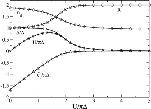
Figure 4: A plot of the renormalized parameters $\tilde{\epsilon}_{d}$, $\tilde{\Delta}$ and $\tilde{U}$ as a function of the bare interaction $U$ for an Anderson model with $\pi\Delta=0.03$ and $\epsilon_{d}=-0.04$. Over this range of $U$ the system moves from a full orbital regime $\epsilon_{d}+U\ll 0$, through an intermediate valence regime $\epsilon_{d}+U\approx 0$, to a localized (Kondo) regime $\epsilon_{d}+U\gg 0$. Also shown are the impurity occupation number $n_{d}$ and the ‘$\chi/\gamma$’ or Wilson ratio R.

The advantage of the renormalized Anderson approach to describe the low energy behaviour of non-degenerate magnetic impurities is that all the parameter regimes; weak coupling, mixed valence, strong correlation, empty and full orbital regimes, can be described precisely within a single framework with, at the most, three renormalized parameters. In Fig. 4 we take values of $U$ over the range $0<U\leq 5\pi\Delta$, with the same values of $\epsilon_{d}$ and $\Delta$ as used earlier. Over this range we move from the full orbital regime for small $U$, through an intermediate valence regime for $\epsilon_{d}+U\sim 0$ and the Kondo regime for $U\gg|\epsilon_{d}|$. We see that $\tilde{\epsilon}_{d}$ increases at first approximately linearly with $U$ until $U/\pi\Delta\sim 2.0$, remaining very close to the Fermi level in the Kondo regime at higher values of $U$. The renormalized resonance width $\tilde{\Delta}$ decreases over the same range monotonically approaching zero in the limit $U\to\infty$. The quasiparticle interaction $\tilde{U}$ increases at first linearly with $U$, reaching a maximum for $U/\pi\Delta\sim 1.5$, and then decreases so that its energy scale merges with that for $\tilde{\Delta}$ in the Kondo regime. The initial increase of $\tilde{\epsilon}_{d}$ with $U$ in the full orbital regime is understandable in terms of the mean field or Hartree-Fock theory, which is approximately valid in this regime. In the mean field theory there is no $\omega$-dependence in the self-energy so $z=1$ and $\tilde{\Delta}_{\rm mf}=\Delta$. There is an effective level given by $\tilde{\epsilon}_{d,{\rm mf}}=\epsilon_{d}+Un_{d,{\rm mf}}/2$, where $n_{d,{\rm mf}}$ is the total impurity occupation calculated within the mean field theory. The value of $\tilde{U}$ in proportional to $U$ for very small $U$, and for larger values of $U$, its value can be estimated from (8) using perturbation theory.[10] These expressions give the general trend as a function of $U$ in the full orbital regime $U\tilde{\rho}_{d,{\rm mf}}\ll 1$ but are not valid as the strong correlation regime is approached, where $\tilde{\Delta}$ begins to differ from the bare value $\Delta$, and breaks down completely in the Kondo regime where $\tilde{\Delta}$ is strongly renormalized (see reference[7] for more extensive results).

Also plotted in Fig. 4 is the Wilson ratio, which is given by $R=1+\tilde{U}\tilde{\rho}_{d}(0)$, and the total impurity occupation number $n_{d}$. The occupation number decreases from 1.88 for $U=0$ to almost 1 in the large $U$ regime, corresponding to localization of the d-electron. The Wilson ratio increases from 1 in the small $U$ regime and asymptotically approaches 2 in the Kondo regime.

4 De-renormalization as a Function of Magnetic Field

If we introduce a magnetic field $H$, we can again generalize the definition of the renormalized parameters, $\tilde{\epsilon}_{d\sigma}$ $\tilde{\Delta}$ and $\tilde{U}$, such that they become functions of the magnetic field $H$. For simplicity we confine the discussion to the particle-hole symmetric model with $\epsilon_{d}=-U/2$. If we absorb the zero field Hartree-Fock contribution to the self-energy, $\Sigma(0,0)=U/2$ then $\epsilon_{d}=0$, and $\Sigma_{\uparrow}(0,h)=-\Sigma_{\downarrow}(0,h)=-\Sigma_{\uparrow}(0,-h)$, where $h=g\mu_{\rm B}H/2$. Eq. (3) gets replaced by

$$\tilde{\epsilon}_{\rm d,{\sigma}}(h)=z(h)(-h\sigma+\Sigma_{\sigma}(0,h)),\quad\tilde{\Delta}(h)=z(h)\Delta,$$ (17)

where $z(h)$ is given by $z(h)={1/{(1-\Sigma^{\prime}_{\uparrow}(0,h))}}$. The occupation of the impurity level is still given by the Friedel sum rule,

$$n_{d\sigma}(h)={1\over 2}-{1\over\pi}{\rm tan}^{-1}\left(\tilde{\epsilon}_{d\sigma}(h)\over\tilde{\Delta}(h)\right).$$ (18)

The definition (8) of $\tilde{U}$ can be straightforwardly generalized to define an field dependent local interaction $\tilde{U}(h)$. As $\tilde{\epsilon}_{d\uparrow}(h)=-\tilde{\epsilon}_{d\downarrow}(h)$, it will be convenient to define a single effective level $\epsilon_{d}(h)$ via $\tilde{\epsilon}_{d}(h)=-\sigma\tilde{\epsilon}_{d\sigma}(h)$. The impurity magnetization $M(h)$ at $T=0$ is then given simply by

$$M(h)={g\mu_{\rm B}\over\pi}{\rm tan}^{-1}\left({\tilde{\epsilon}_{d}(h)\over\tilde{\Delta}(h)}\right).$$ (19)

The expressions given earlier for the quasiparticle density of states (5), impurity spin and charge susceptibilities (12), and specific heat coefficient (6) can be generalized to include the magnetic field dependence by replacing $\tilde{\epsilon}_{d}$, $\tilde{\Delta}$ and $\tilde{U}$, by $\tilde{\epsilon}_{d}(h)$, $\tilde{\Delta}(h)$ and $\tilde{U}(h)$.

The simplest way to calculate the field dependent renormalized parameters using the NRG for the particle-hole symmetric model is to exploit the spin-isospin symmetry of the model, which is such that the symmetric model in a magnetic field with positive-$U$ is equivalent to a negative-$U$ asymmetric model in the absence of a magnetic field with $\epsilon_{d}+U/2=-h$ and spin and charge (isospin) interchanged. Calculations can then be carried out in the absence of a magnetic field using the asymmetric model with negative-$U$. The isospin symmetry of the particle-hole symmetric model is then effectively exploited via the spin symmetry. This has two advantages, it enables one to retain more states in the NRG iterations, and requires no modification of the standard NRG program.

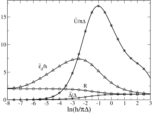
Figure 5: The renormalized parameters $\tilde{\epsilon}_{d}(h)/h$. $\tilde{\Delta}(h)/\Delta$, $\tilde{U}(h)/\pi\Delta$ and the Wilson ratio $R(h)$ plotted as a function of the logarithm of the magnetic field $h/\pi\Delta$ for the symmetric Anderson model with $U/\pi\Delta=5$, $\pi\Delta=0.03$, and a bandwidth $2D=2$. The parameters vary from the strong correlation values in weak field, $\pi\tilde{\Delta}(0)=\tilde{U}(0)$, $R(0)=2=\lim_{h\to 0}\tilde{\epsilon}_{d}(h)/h$, to those of the bare model, $\tilde{U}(h)=U$, $\tilde{\Delta}(h)=\Delta$, $R(h)=1=\tilde{\epsilon}_{d}(h)/h$ in fields $h\gg U$.

In Fig. 5 we give the results for $\tilde{\epsilon}_{d}(h)/h$, $\tilde{\Delta}(h)/\Delta$ and $\tilde{U}(h)/\pi\Delta$ as a function of $h$ for the symmetric model with $U/\pi\Delta=5$, which corresponds to a Kondo temperature $T_{\rm K}/\pi\Delta=0.00204$. We can follow the gradual de-renormalization of the quasiparticles as the magnetic field increases. In weak field $\tilde{\epsilon}_{d}/h\to 2$ as $h\to 0$, so the level splitting in a magnetic field of the local spin-up and spin-down states is twice the Zeeman splitting for free quasiparticles. This enhancement factor of 2 is the same as that for the Wilson or $\chi/\gamma$ ratio. As the magnetic field strength increases $\tilde{\epsilon}_{d}(h)/h$ increases to a maximum, and only for magnetic field strengths larger than $h\gg U$ does this ratio finally approach the free particle value, $\tilde{\epsilon}_{d}(h)/h\to 1$. There is an even more dramatic increase in the value of $\tilde{U}(h)/\pi\Delta$. For $h\to 0$ we are in the strong correlation or Kondo limit, $\tilde{U}(0)/\pi\Delta(0)=4T_{\rm K}/\pi\Delta$, so the value of $\tilde{U}(h)$ is small in the weak field regime. However, it increases significantly with an increase of field strength to a maximum, approximately three times greater than the bare value of 5, before eventually approaching the bare value for $h\gg U$.

The fact that the quasiparticle interaction becomes very large does not imply that the effects of the interaction become stronger; the contrary is the case. A more significant measure of the effect of the interactions is the product of $\tilde{U}(h)$ with the quasiparticle density of states at the Fermi level $\rho_{d}(0,h)$. The increase in $U(h)$ is more than compensated by the fall off of $\rho_{d}(0,h)$ with $h$ as the level moves away from the Fermi level. This can be seen from the Wilson ratio $R(h)=1+\tilde{\rho}_{d}(h)\tilde{U}(h)$, which is also shown in Fig. 5. The value of $R$ decreases monotonically from the strong correlation value 2 to the free particle value 1 in the extreme large field limit $h\gg U$, which implies that the product $\tilde{\rho}_{d}(h)\tilde{U}(h)$ is always less than 1. The enhanced value of $\tilde{U}(h)$ in the strong magnetic field limit, and the decrease as $h\to\infty$, is understandable in terms of mean field theory, where from eq. (8) $\tilde{U}(h)$ is given by

$$\tilde{U}_{\rm mf}(h)={U\over 1-U\tilde{\rho}_{d,{\rm mf}}(0,h)},$$ (20)

as $\tilde{\rho}_{d,{\rm mf}}(0,h)$ decreases with increase of $h$ in this regime.

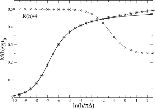
Figure 6: The induced impurity magnetization $M(h)$ (stars and dashed curve) as a function of ${\rm ln}(h/\pi\Delta)$ for the symmetric Anderson model with the same parameter set as used in Fig. 5 ($U/\pi\Delta=5$) compared with the same values from the Bethe ansatz solution[14, 15] of the s-d model (full curve). Also shown is the Wilson ratio $R(h)$ divided by 4 (crosses and dotted line).

In Fig. 6 we plot the impurity magnetization as function of the logarithm of $h$ using the non-interacting quasiparticle expression in eq. (19) using the parameters $\tilde{\epsilon}_{d}(h)$ and $\tilde{\Delta}(h)$ given in Fig. 5, together with the corresponding values for an s-d model with the same Kondo temperature[15]. Also plotted in the same Fig. is $R(h)/4$. One sees that there is complete agreement with the results of the s-d model until charge fluctuations begin to play a role for $h\sim\pi\Delta$ (${\rm ln}(h/\pi\Delta)\sim-3$). Up to this point $R(h)\approx 2$ ($\tilde{U}(h)\tilde{\rho}_{d}(0,h)\approx 1$) independent of $h$, as is well known for the s-d model[15, 16], but then crosses over eventually to the free electron value $R(h)=1$ for $h\gg\pi\Delta$. The magnetization can be seen to approach saturation more rapidly with $h$ than predicted from the s-d model, due to the additional effect of the charge fluctuations.

The calculation of the magnetization from eq. (19) does not depend on the quasiparticle interaction $\tilde{U}(h)$, but the formula for the susceptibility in eq. (12) as a function of $h$ does. A check on the values of $\tilde{U}(h)$ can be made by calculating the susceptibility from eq. (12) using $\tilde{\epsilon}_{d}(h)$, $\tilde{\Delta}(h)$ and $\tilde{U}(h)$, and comparing the result with that calculated by numerically differentiating the results for $M(h)$. When this check is made complete consistency is found, confirming the calculated values of $\tilde{U}(h)$.

5 Perturbation Expansion with Running Coupling Constants

The values of $\tilde{\epsilon}_{d}(h)$, $\tilde{\Delta}(h)$ and $\tilde{U}(h)$ obtained in the previous section provide a set of running coupling constants for a renormalized perturbation expansion for the symmetric Anderson model in a magnetic field. Instead of working with $\tilde{\Delta}$ and $\tilde{U}$ of the model in the absence of a magnetic field, the perturbation expansion can be carried out using parameters appropriate to the field strength $h$. If the calculations could be carried out exactly then it would not matter which set of coupling constants is used, as the model is completely defined by any one set. However, for approximate calculations in the low energy regime the best set in the presence of a magnetic field $h$ must be the set $\tilde{\epsilon}_{d}(h)$, $\tilde{\Delta}(h)$ and $\tilde{U}(h)$, because low order calculations in terms of these parameters give asymptotically exact results as $T\to 0$.

We apply this approach to the calculation of the low temperature conductivity in the presence of a magnetic field for the particle-hole symmetric model $\sigma(T,h)$. The calculation is along the same lines as that used to derive the $h=0$ result in eq. (13)[9]. All the terms in the RPT expansion to order $\tilde{U}(h)^{2}$ are taken into account, including the counter terms to this order. The result, when summed over the two spin components, can be written in the form,

$$\sigma(h,T)={\sigma_{0}\over{\rm cos}^{2}m(h)}\left\{1+\sigma_{2}(h)\left(T\over T_{\rm K}\right)^{2}+{\rm O}((T/T_{\rm K})^{4})\right\},$$ (21)

where $m(h)=\pi M(h)/g\mu_{\rm B}$ and the coefficient $\sigma_{2}(h)$ is given by

$$\sigma_{2}(h)={\pi^{3}\tilde{\rho}_{d}(0,h)\tilde{\Delta}^{2}(0)\over{48\tilde{\Delta}(h)}}\left\{1+2\pi\tilde{\Delta}(h)\tilde{U}^{2}(h)\tilde{\rho}_{d}^{3}(0,h)\right\}$$

$$={\pi^{2}{\rm cos}^{2}m(h)\tilde{\Delta}^{2}(0)\over{48\tilde{\Delta}^{2}(h)}}\left\{1+2[R(h)-1]^{2}{\rm cos}^{2}m(h)\right\}.$$ (22)

This result is exact to order $T^{2}$ if either $h$ or $U$ is set to zero, and we conjecture, that it is exact for the general case $U\neq 0$ and $h\neq 0$. In Fig. 7 we plot the logarithm of the coefficient $\sigma_{2}(h)$ of the $T^{2}$ term as a function of $h$ over a range from strongly correlated quasiparticles in weak field to bare quasiparticles in fields $h\gg U$, using the renormalized parameters shown in Fig. 6 for the model with $U/\pi\Delta=5$. In Fig. 8 we plot $\sigma_{2}(h)$ for a more realistically obtainable range of $h$, $0<h<1.5T_{\rm K}$, for the same model where $T_{\rm K}/\pi\Delta=0.00204$. There is a very significant decrease in this coefficient over this magnetic field range.

This RPT calculation has had to rely on the renormalized parameters derived from the NRG energy levels. It might, however, be possible to calculate them directly from eqs. (3) and (10), using an iterative RPT. In the asymptotically large field limit, the parameters are those of the bare model, but the interaction effects are small because the impurity is almost completely polarized. It should be possible, therefore, to use perturbation theory for the bare model to calculate the small renormalization effects for large $h$, and the set of renormalized parameters for this regime. With these new set of renormalized parameters, the RPT could be then used to calculate the renormalized parameters for slightly smaller fields, and enabling one to set up flow equations to continue the process to the small field regime. The perturbation effects at each stage should be small, as the effects of only small changes in the magnetic field will be calculated at each stage, and there are only three parameters, $\tilde{\epsilon}_{d}$, $\tilde{\Delta}$ and $\tilde{U}$, to consider, as these three fully specify the expansion.

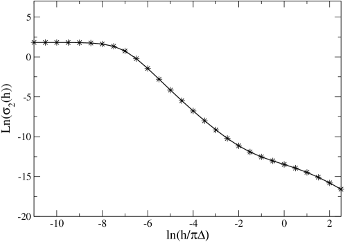
Figure 7: The logarithm of $\sigma_{2}(h)$ (stars), the coefficient of the $(T/T_{\rm K})^{2}$ term in the expression (21) for the low temperature conductivity $\sigma(T,h)$, is plotted as a function of the logarithm magnetic field $h$ using the renormalized parameters shown in Fig. 6 (symmetric model with $U/\pi\Delta=5$)

.

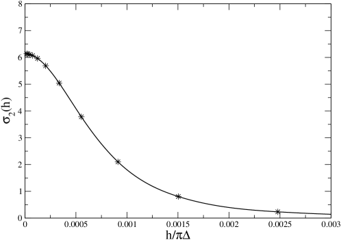
Figure 8: The coefficient of the $(T/T_{\rm K})^{2}$ term (stars) in the expression (21) for the low temperature conductivity $\sigma(T,h)$ is plotted as a function of the magnetic field $h$ over a range $0<h<1.5T_{\rm K}$, using the renormalized parameters shown in Fig. 6 (symmetric model with $U/\pi\Delta=5$, $T_{\rm K}/\pi\Delta=0.00204$)

.

It might also be possible to do something similar as a function of temperature starting with the high temperature limit, progressively lowering the temperature, hence having running parameters, $\tilde{\epsilon}_{d}(T)$, $\tilde{\Delta}(T)$ and $\tilde{U}(T)$. We have explored this possibility by taking the parameters, $\tilde{\epsilon}_{d}(N)$, $\tilde{\Delta}(N)$ and $\tilde{U}(N)$ as a function of $N$, and translating these into parameters for a temperature scale, $T_{N}=\eta D\Lambda^{-(N-1)/2}$, where $\eta$ is an appropriately chosen constant of order unity[7]. For the particle-hole symmetric case we take the value of $\tilde{U}_{pp}(N)$ (=$\tilde{U}_{hh}(N)$) as $\tilde{U}(N)$, and translate this, together with $\tilde{\Delta}(N)$ and $\tilde{\epsilon}_{d}(N)$, into parameters appropriate for a temperature scale $T_{N}$, and generalize the RPT expression for the impurity susceptibility in eq. (12) to finite temperatures,

$$\chi_{s}(T)={(g\mu_{\rm B})^{2}\over 2}\tilde{\rho}_{d}(0,T)(1+\tilde{U}(T)\tilde{\rho}_{d}(0,T)),$$ (23)

where $\tilde{\rho}_{d}(0,T)$ is the free quasiparticle contribution to the impurity susceptibility given by

$$\tilde{\rho}_{d}(0,T)=-\int_{-\infty}^{\infty}\tilde{\rho}_{d}(\omega){\partial f(\omega)\over\partial\omega}d\omega$$ (24)

where $f(\omega)=1/(e^{\omega/T}+1)$, and $\tilde{\rho}_{d}(\omega)$ is the free quasiparticle density of states given by eq. (5). We calculate $\tilde{\rho}_{d}(0,T)$ in the Kondo regime for $U/\pi\Delta=5.0$ at values of $T_{N}$, using the renormalized parameter $\tilde{\Delta}(T_{N})$, with $\tilde{\epsilon}_{d}(T_{N})=0$ and $\eta=1.2$, as is used in the NRG evaluation of spectral densities on a scale $\omega_{N}$ (see for example [17, 18]). We then deduce $\chi_{s}(T)$ from eq. (23) using $\tilde{U}(T_{N})$. In Fig. 9 we compare the results of this calculation with the Bethe ansatz results for the s-d model given in reference [15]. There is excellent agreement with the exact Bethe ansatz results over this temperature range. The enhanced value of $\tilde{U}(T)$ at very high temperatures, as in the high field case, is qualitatively understandable in terms of mean field theory, where $\tilde{U}_{\rm mf}(T)={U/(1-U\tilde{\rho}_{d,{\rm mf}}(0,T)})$, which when substituted into eq. (12) gives the mean field value for $\chi_{s}(T)/(g\mu_{\rm B})^{2}=0.5\tilde{\rho}_{d,{\rm mf}}(0,T)/(1-U\tilde{\rho}_{d,{\rm mf}}(0,T))$. The value of $\chi_{s}(T)/(g\mu_{\rm B})^{2}$ in the extreme high temperature range corresponds to that of the free bare model, $1/8T$. It can be seen from Figs. 1 and 2 that in the smaller $N$ range there is no unique prediction for $\tilde{U}(N)$, so this calculation is not well defined. Nevertheless, the agreement with the Bethe ansatz results is remarkable and it does indicate that an RPT expansion with temperature dependent parameters might be possible. Such a perturbation expansion, being a general technique, would have a potentially wide application to other strongly correlated systems.

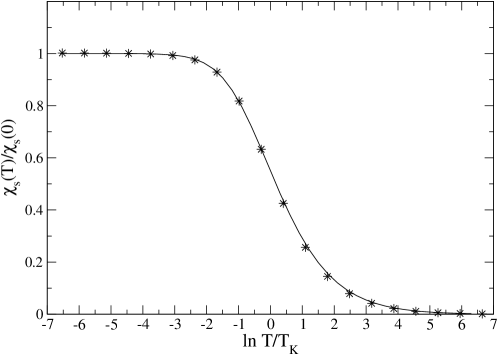
Figure 9: The ratio of $\chi_{s}(T)/\chi_{s}(0)$ (stars) deduced from eq. (23) using temperature dependent parameters $\tilde{\Delta}(T)$ and $\tilde{U}(T)$, for the symmetric model with $U/\pi\Delta=5$ as a function of the temperature $T$. The full curve is that derived from the Bethe ansatz solution of the s-d model[15].

6 Conclusions

We have shown that low energy or strong coupling NRG fixed point of the s-d and Anderson models can be analysed as a renormalized version of the Anderson model. This analysis has the advantage that the Fermi liquid aspects, and the 1-1 correspondence of the single particle excitations with those of the non-interacting system, is brought out clearly. The three renormalized parameters, $\tilde{\epsilon}_{d}$, $\tilde{\Delta}$ and $\tilde{U}$, can be used to specify completely a renormalized perturbation expansion, which is applicable on all energy scales.

With a magnetic field present, renormalized parameters, $\tilde{\epsilon}_{d}(h)$, $\tilde{\Delta}(h)$ and $\tilde{U}(h)$ have been calculated as a function of the magnetic field strength $h$. Using these parameters in the renormalized perturbation theory, we have derived an expression for the low temperature conductivity as a function of magnetic field strength.

References

- [1] K.G. Wilson, Rev. Mod. Phys. 47 (1975) 773.
- [2] P. Nozières, J. Low Temp. Phys. 17 (1974) 31: Low Temperature Physics Conference Proceedings LT14
- [3] The full definition of this ratio is .
- [4] P.W. Anderson, Phys. Rev. 124 (1961) 41.
- [5] J. Friedel, Can. J. Phys. 54 (1956) 1190; J.M. Langer and V. Ambegaokar, Phys. Rev. 164 (1961) 498; D.C. Langreth, Phys. Rev. 150 (1966) 516.
- [6] H.R. Krishnamurthy, J.W. Wilkins and K.G. Wilson, Phys. Rev. B 21 and 1044 (1980) 1003.
- [7] A.C. Hewson, A. Oguri and D. Meyer, cond-mat/0312484 (2003); to be published Eur. Phys. J B (2004).
- [8] See for example, N.N. Bogoliubov and D.V. Shirkov, Introduction to the Theory of Quantized Fields (Wiley-Interscience, New York, 1980).
- [9] A.C. Hewson, Phys. Rev. Lett. 70 (1993) 4007.
- [10] A.C. Hewson, J. Phys. Condens.-Matter, 13 (2001) 10011.
- [11] D.M. Newns and A.C. Hewson, J. Phys. F 10 (1980) 2429.
- [12] K. Yamada, Prog. in Theor. Phys., 53 (1975) 1970;ibid. 54 (1975) 316; K. Yosida and Y. Yamada, ibid. 53 (1975) 1286.
- [13] A. Oguri, Phys. Rev. B 64 (2001) 153305: see also the contribution from Oguri in this volume.
- [14] N. Andrei, K. Furuya and J.H. Lowenstein, Rev. Mod. Phys. 55 (1983) 331.
- [15] A.M. Tsvelick and P.B. Wiegmann, Adv. Phys. 32 (1983) 453.
- [16] The Fermi liquid relation can be seen to hold from eqs. (6) and (12). In the localized regime is negligible and it then follows from [3] that .
- [17] O. Sakai, Y. Shimizu and T. Kasuya J. Phys. Soc. Jap. 58 (1989) 3666.
- [18] T. A. Costi, A.C. Hewson and V. Zlatić, J. Phys.: Condens. Matter 6 (1994) 2519.