Stability in the evolution of random networks

Abstract

With a simple model, we study the evolution of random networks under attack and reconstruction. We introduce a new quality, invulnerability $I(s)$, to describe the stability of the system. We find that the network can evolve to a stationary state. The stationary value $I_{c}$ has a power-law dependence on the initial average degree $\langle k\rangle$, with the slope is about $-1.485$. In the stationary state, the degree distribution is a normal distribution, rather than a typical Poisson distribution for general random graphs. The clustering coefficient in the stationary state is much larger than that in the initial state. The stability of the network depends only on the initial average degree $\langle k\rangle$, which increases rapidly with the decrease of $\langle k\rangle$.

I Introduction

Many systems can be represented by networks, a set of nodes joined together by links indicating interactions. Social networks wasserman , the Internet BA1 , food webs williams , transportation networks Li ; Chi ; Latora , and linguistic networks Cancho are just some examples of such systems. The investigation of complex networks was initiated by Erdős and Rényi ER1 . They proposed and studied one of the earliest theoretical models of a network, the random graph. In a random graph, $N$ labelled nodes are connected by $n$ edges, which are chosen randomly from the $N(N-1)/2$ possible edges. It is trivial to show that the connection probability is $p=n/[N(N-1)/2]$. The number $k$ of edges connecting one node to others is called the degree of that node. The average degree of the graph is $\langle k\rangle=2n/N=p(N-1)\simeq pN$ if $p\ll 1$. The degree distribution for a random network is given by a Poissonian distribution.

Recently the increasing accessibility of databases of real networks and the availability of powerful computers have made possible a series of empirical studies on complex networks. Thus, other two main streams of topics were proposed and investigated in depth. One is the small-world networks introduced by Watts and Strogatz WS1 ; WS2 . Such networks are highly clustered like regular lattices, yet have small characteristic path lengths like random graphs. The other is the scale-free networks proposed by Barabási and Albert BA2 ; BA3 ; BA4 , based on two generic mechanisms, growth and preferential attachment. Those networks have scale-free power-law degree distributions.

With increased threats of hacker attacks and routers malfunction, etc., research in the field of network robustness has attracted much attention attack1 . Albert and his collaborators have shown that scale-free networks, at variance with random graphs and small-world networks, are almost unaffected by errors while vulnerable to attacks. That is, the ability of their nodes to communicate is almost unaffected by the failure of some randomly chosen nodes, but the removal of a few most connected nodes can damage the networks. Recently the network efficiency of errors and attacks on scale-free networks has also been studied efficiency . In those studies, the damaged nodes are removed from the network. Thus the size of the network decreases with the evolution of the system.

Based on the physics of network tolerance, using a simple model on evolving network, we are trying to study the robustness of a dynamical evolving network. We will consider the reconstruction of the links of the damaged nodes instead removing the nodes from the network. Thus the size of the system remains unchanged. This is more closer to the evolution of real networks. The paper is organized as follows. The evolution model is presented in next section. Section III is devoted to analyze the results of the model, along with a definition of how we describe the stability of the network. In last section we conclude and give a brief discussion.

II An Evolution Model

Despite the fine work of studies on network tolerance, little effort has been made on the reconstruction of the attacked network. The aim of our model is to investigate the stability of the network during the evolution in terms of attacks and reconstructions. In other words, the nodes damaged will not be removed from the network, instead they will be reconnected in certain way. Assume that all information on the former links of the damaged nodes has been lost, the damaged nodes have to be connected randomly to other nodes in the network again. In this way, we keep the size of the system constant. We do not try to consider a case with increasing size in the evolution, since the process of system’s size increase can be much slower than the frequently happening damage and reconstruction. We try to investigate the effect of such a reconstruction on the evolution of the network. For this purpose, we first setup a random netweok with $N$ nodes and connection probability $p$, then let the network evolve according to the following rules: (i) Find the node with the highest degree $k_{max}$. Since this node has highest connections to other nodes, it is most likely attacked and is the most vulnerable site in the network. For simplicity, we assume that only a node with highest connections suffers attack and to be reconnected. If several nodes happen to have the same highest degree of connection, only one (randomly chosen) of them is assumed to be damaged in the attack. (ii) Reconnect this node with the other nodes in the network with the reconstruction probability $p_{re}=p$. Steps (i) and (ii) are repeated to a prefixed number of times. This number should be large enough to enable the system to reach (possibly existing) stationary state. In our simulation, it is chosen to be 10 million. The reconnection process represents the effort of reconstructing the network. We set the reconnection probability $p_{re}$ the same as the initial construction probability $p$ to reduce the number of parameters in the model. This set also implies that the information does not increase from initial construction to later reconnection. Thus, the evolution of the network is in fact a process of bing damaged and subsequent reconstructing, similar to the evolution of real networks.

The interest in our model investigation is to find out whether there exists a stationary state in the evolution of the network, and if it exists, what are the properties of the stationary state and their dependences on the parameters in the model.

III Simulation Results

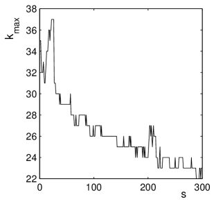
Figure 1: Plots of $k_{max}$ versus step $s$ with $N=1000$, $p_{re}=p=0.02$.

The model defined in Sect. II has several nontrivial consequences. It can be easily seen that the network has a tendency to decrease the maximum number of connections among the nodes at a long time scale, because the nodes with highest connections will be damaged and reconnected randomly. From the evolution rules, the total number of connections in the network will also decrease generally before a stationary state is reached.

To get some idea on the safety of the network, we can have a look at the behavior of the maximum degree of connection of the network. In Fig. 1, we give a snapshot of the maximum degree $k_{max}$ versus time step $s$ for a network with $N=1000$ nodes and connection probability $p_{re}=p=0.02$. Apart from some fluctuations, it decreases in the evolution. From intuition, a node with less links to others will be attacked less frequently. Thus a network with smaller maximum connection degree is safer. To describe the safety of the network, we introduce a new quantity, the invulnerability $I(s)$, which is analogous in definition to the gap $G(s)$ in the Bak-Sneppen model BS1 ; BS2 . Considering an evolution of network with maximum degrees $k_{\rm max}(1),k_{\rm max}(2),\cdots,k_{\rm max}(s)$, invulnerability $I(s)$ at time $s$ is defined

$$I(s)=1/Min\{k_{\rm max}(i)\}\ \ \textbf{for\ \ \ }i\leq s\ ,$$ (1)

i.e., the inverse of the minimum of all the maximum degrees in the evolution before moment $s$. Initial value of $I(s)$ is equal to $1/k_{max}(1)$. $I(s)$ reflects the attack tolerance of the network. When $I(s)$ is small, the network is vulnerable to attack. Obviously from definition, $I(s)$ is a non-decreasing function of evolution, and some fluctuations in $k_{\rm max}$ have been filtered out.

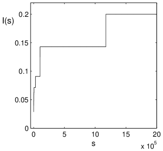
Figure 2: Plots of invulnerability $I(s)$ versus $s$ for network with $N=1000$ nodes and connection probability $p_{re}=p=0.02$.

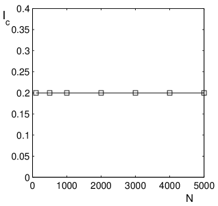
Figure 3: The stationary value of $I_{c}$ as a function of network size $N$ when $\langle k\rangle=20$ fixed.

Fig. 2 shows $I(s)$ versus step $s$ with network size $N=1000$ and probability $p_{re}=p=0.02$. We observe that $I(s)$ increases very quickly at small $s$ but slowly at large $s$ and finally reaches a constant value when $s$ is large enough. The increase of $I(s)$ indicates that the system is getting more and more safe in general by experiencing continuous attacks and reconstructions. This figure is similar to the envelope function of Bak-Sneppen evolution model. Without interference from outside world, the network evolves to a stationary state. And the process takes place over a very long transient period. In Fig. 3, we present the stationary value $I_{c}$ as a function of the network size $N$ under a fixed initial average degree $\langle k\rangle=20$. We find $I_{c}$ stays unchanged at 0.2 with $N$ shifted from 100 to 5000. This result is interesting, because it shows that the stationary value $I_{c}$ depends not on the network size $N$ and probability $p_{re}=p$ separately but through the initial average degree $\langle k\rangle=pN$. Such a dependence can be expected considering the facts that the initial degree distribution has an average $\langle k\rangle=pN$ with variance $\sigma^{2}=\langle k\rangle=pN$ and that the average number of links to the reconstructed nodes is also $\langle k\rangle=pN$. As a result, the properties of the evolution are mainly determined by the value of initial average degree $\langle k\rangle=pN$. To get the relationship between $I_{c}$ and $\langle k\rangle$ we show in Fig. 4 $I_{c}$ as a function of $\langle k\rangle$ in a log-log plot. We find that $I_{c}$ has a power-law dependence on the average degree $\langle k\rangle$,

$$I_{c}(\langle k\rangle)\propto{\langle k\rangle}^{-\tau},$$ (2)

where the exponent $\tau$ is about 1.485. Fig. 4 illustrates that after the network has relaxed to the stationary state, the stability of the network will increase rapidly with the decrease of average degree $\langle k\rangle$ in the initial state. Thus, when the initial average degree $\langle k\rangle$ is small, i.e., less communications and interactions in the network, the system will be more stable. We would like to mention that the value of $\tau=1.485$ results from the nonlinear interactions among the nodes.

Figure 4: $\ln I_{c}$ versus $\ln\langle k\rangle$. A linear fit is shown as dash line with slope $-1.485$.

In order to offer a further information of the network in the stationary state, one can compare some structural properties of the network in the initial state with those in the stationary state.

Because of the reconnection of a damaged node to other randomly chosen ones, the nodes with modest degree of connection may increase their links. As a result of the reconstruction, the distribution of connections $k$ changes in the evolution of the system. To see how dramatically the change is, we compare the distributions at initial state and the state in which $I(s)$ remains unchanged. For this purpose, we construct a random graph with $N=10000$ nodes and $p=0.005$ and plot its degree distribution in the initial state by circles in Fig. 5(a). Because of the randomness of the initial connections, the initial degree distribution of a random graph is a Poisson distribution for large $N$ BA4 ,

$$P(k)=e^{-\langle k\rangle}\langle k\rangle^{k}/k!\,$$ (3)

with peak at about $\langle k\rangle=50$. This theoretical expectation is shown in the figure as the solid line. Then let the network evolve with the given simulation rules. When the system reaches the stationary state, we draw its degree distribution, as represented by squares in Fig. 5(a). We fit the distribution to a normal distribution, and find that the average degree is $\langle k\rangle=17$ and standard deviation is $\sigma=7$. One can see that the mean degree of connection decreases by a factor 3 in the evolution. One may notice that a Poissonian distribution can be approximated by a normal distribution when the mean value $\langle k\rangle$ is large. For Poissonian distribution, the width of the distribution is determined also by the mean value $\langle k\rangle$ as $\sigma=\sqrt{\langle k\rangle}$. In a normal distribution, the width has no correlation with its mean value. Therefore, the stationary degree distribution can not be described by a Poissonian distribution. To investigate the dependence of such a change on the initial $\langle k\rangle$, we do the same investigation for a network with $N=10000$ nodes and $p=0.015$. This time, the initial $\langle k\rangle$ is 150. The initial and final state distributions of connection are shown in Fig. 5(b), represented by circles and squares, respectively. Both distributions can be fitted very well by Gaussian distributions, with $\langle k\rangle=150$ for the initial distribution as expected and 77 for the final state. The width of the final state connection distribution is now $\sigma=18.5$. From these two evolutions one can conclude that the change of connection distributions depends on the initial mean degree nontrivially. The higher the initial mean degree, the wider of the distribution for the stationary state. In fact, the two average degrees above in the stationary states satisfy the relation in Eq. (2) with the same $\tau$ for $I_{c}$. One more observation is that the relative width $\sigma/\langle k\rangle$ of the distributions increases by a factor of about 3 in the evolution for different initial average degree $\langle k\rangle$. Because of the constant factor in the change of relative width in the evolution, the width for the stationary state can be smaller or larger than that in the initial state, depending on the value of initial average degree.

Another feature with the evolution of the network is the emergence of isolated nodes. When the only one link a node has is a connection to the node with highest degree under attack, the node may have no connection to the network and becomes isolated after reconstruction. Needless to say, the number of isolated nodes depends on the evolution stage and the value of initial average degree $\langle k\rangle$. The larger the initial average degree $\langle k\rangle$, the less the number of isolated nodes at fixed steps since the evolution. Our simulation shows that the probabilities for a node to be isolated in the stationary state are 0.03$\%$ and 25$\%$ with initial degree $\langle k\rangle=$ 50 and 15, correspondingly. When initial mean degree $\langle k\rangle$ is small, many nodes are isolated, and the isolation of many nodes makes the nodes more independent and the system more stable.

An important property of a network is its clustering coefficient. To know the behavior of the clustering coefficient in the evolution, we need to calculate the clustering coefficient of the network in the initial state and in the stationary state. Let us focus first on a selected node $i$ of the network. Suppose the node have $k_{i}$ edges connecting its so-called nearest neighbors. The maximum possible edges among $k_{i}$ nearest neighbors is $k_{i}(k_{i}-1)/2$. We use $n_{i}$ to denote the number of edges that actually exist among those neighbors. The clustering coefficient of node $i$ is defined as:

$$C_{i}=\frac{n_{i}}{k_{i}(k_{i}-1)/2}.$$ (4)

The clustering coefficient of the entire network is defined as the average over the whole network,

$$C=\frac{1}{N}\sum_{i}C_{i}.$$ (5)

We find that the clustering coefficient in the stationary state is much larger than that in the initial state. For a network with $N=10000$ nodes, the clustering coefficients in the initial state are equal to 0.005 and 0.015 when the initial mean degrees $\langle k\rangle$ are 50 and 150, respectively, while the clustering coefficients in the stationary state are 0.23 and 0.1, respectively.

From the fact that the network in the stationary state has the large clustering coefficients together with some isolated nodes and low average degrees, one can conclude that the system is driven in its evolution to a state composed of quite a few highly clustered small clusters. This is in sharp contrast with the network in the initial state when the system has a small clustering coefficient, almost no isolated nodes, and a high average degree.

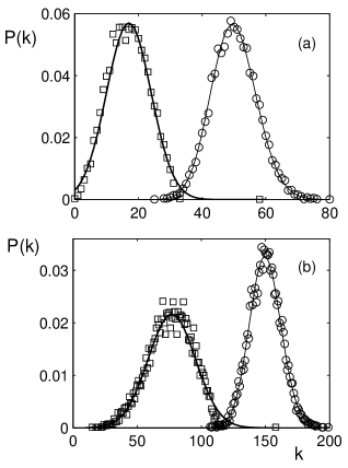
Figure 5: A comparison of degree distributions of the network in the initial state (circles) with that in the stationary state (squares) for (a) $N=10000$ and $p=0.005$; (b) $N=10000$ and $p=0.015$. Solid lines are Gaussian fits.

IV Discussions and Conclusions

In this paper, we study the evolution of random networks under continuous attacks and subsequent reconstructions. We introduce a new quality, invulnerability $I(s)$, to describe the safety of the network. A stationary state with fixed $I(s)$ is observed during the evolution of the network. The stationary value of invulnerability $I_{c}$ is found to be independent of the network size $N$ and the probability $p_{re}=p$ when the initial average degree is fixed. $I_{c}$ shows a power-law dependence on the initial mean degree $\langle k\rangle$, with the exponent is about $-1.485$.

We give further information on the evolution of the properties of the network. The first property is the evolution of the degree distribution. The degree distributions of a network in both the initial and the stationary states are found to be normal distributions. After evolution, the peak position in the distribution shifts to lower connection degree while the relative width $\sigma/\langle k\rangle$ increases considerably. In the stationary state, the edges and degrees in the whole network decrease a lot and quite a few isolated nodes appear. The second is the clustering coefficient. The clustering coefficient of a network in the stationary state is much larger than that in the initial state.

In summary, the stability of the network is found to be related closely to the initial average degree $\langle k\rangle$ and has little correlation with the network size $N$ and probability $p_{re}=p$ separately. The stability of the network will increase rapidly with the decrease of initial average degree $\langle k\rangle$. The reason is that when $\langle k\rangle$ is small, the edges and degrees decrease a lot and more isolated nodes appear, which weaken the ability of nodes to communicate with each other and make the network more stable. From the isolated nodes and high clustering coefficient, we conclude that the network in the stationary state is composed of some highly clustered small clusters.

Still, there are many issues to be addressed, such as the correlations and the fluctuations in $k_{max}$ in the evolution, especially after the stationary state. These fluctuations may tell us more the nature of the stationary state. The behavior of the average degree in the evolution also may shed some light on the dynamics of network. In addition, it is worthwhile to investigate whether the evolution of random networks demonstrate self-organized criticality (SOC), according to the similarity between the evolution of invulnerability $I(s)$ with that of the envelope function $G(s)$ in Bak-Sneppen model. All these topics can not be covered in this paper, and will be discussed later.

References

- (1) S. Wasserman and K. Faust, Social Network Analysis, (Cambridge University Press, Cambridge, England, 1994).
- (2) R. Albert, H. Jeong, and A.-L. Barabási, Nature 401, 130 (1999).
- (3) R. J. Williams and N. D. Martinez, Nature 404, 180 (2000).
- (4) W. Li and X. Cai, Phys. Rev. E 69, 046106 (2004).
- (5) L. P. Chi, R. Wang, H. Su, et al, Chin. Phys. Lett. 20, 1393 (2003).
- (6) V. Latora and M. Marchiori, Physica A 314, 109 (2002).
- (7) R. F. Cancho and R. V. Solé, Proc. Natl. Acad. Sci. 100, 788 (2003).
- (8) P. Erdős and A. Rényi, Publ. Math. Inst. Hung. Acad. Sci. 5, 17 (1960).
- (9) D. J. Watts and S. H. Strogatz, Nature 393, 440 (1998).
- (10) D. J. Watts, Small Worlds: The Dynamics of Networks between Order and Applications, (Princeton University Press, Princeton, New Jersey, 1999).
- (11) A.-L. Barabási and R. Albert, Science 286, 509 (1999).
- (12) A.-L. Barabási, R. Albert, and H. Jeong, Physica A 281, 69 (2000).
- (13) R. Albert and A.-L. Barabási, Rev. Mod. Phys. 74, 47 (2002).
- (14) R. Albert, H. Jeong, and A.-L. Barabási, Nature 406, 378 (2000).
- (15) P. Crucitti, V. Latora, M. Marchiori, and A. Rapisarda, Physica A 320, 622 (2003).
- (16) P. Bak and K. Sneppen, Phys. Rev. Lett. 71, 4083 (1993).
- (17) M. Paczuski, S. Maslov, and P. Bak, Phys. Rev. E 53, 414 (1996).