Currents in a many-particle parabolic quantum dot under a strong magnetic field

Abstract

Currents in a few-electron parabolic quantum dot placed into a perpendicular magnetic field are considered. We show that traditional ways of investigating the Wigner crystallization by studying the charge density correlation function can be supplemented by the examination of the density-current correlator. However, care must be exercised when constructing the correct projection of the multi-dimensional wave function space. The interplay between the magnetic field and Euler-liquid-like behavior of the electron liquid gives rise to persistent and local currents in quantum dots. We demonstrate these phenomena by collating a quasi-classical theory valid in high magnetic fields and an exact numerical solution of the many-body problem.

I Introduction

The problem of the electronic structuremaks00 ; kouw01 ; reimann02 of few-electron quantum dotsjacak98 still remains in the center of attention of solid state research. Although recently substantial achievements have been made by relying on the exact numerical solutionmaarten03 ; yang02 ; mikh01 of the complicated quantum-mechanical problem, simplified approachesvas02 and simple analytical models are also of great interest and even become increasingly more popular.lent91 ; tan99 ; mat94 ; yann02 ; yann03 ; anis04 Besides their relative simplicity, these models are attractive due to the provided physical insight and transparent visualization of the relevant phenomena.

The successful development of the approximation based on the picture of a rotating electron moleculeyann02 ; yann03 encouraged us to look at the rotation in quantum dots more closely. Namely, we investigated the distribution of currents in the simplest quantum dot — the rotating electron ring formed in a few-electron system in a parabolic confinement and a perpendicular magnetic field.

Bedanov and Peetersbedanov94 predicted the crystallization of a system of classical two-dimensional (2D) particles in an external parabolic confinement into a set of concentric rings. In quantum dots containing up to five electrons only one ring is formed. An accurate quantum-mechanical solution based e. g. on the exact numerical diagonalization of the many-electron Hamiltonian provides a circularly symmetric distribution of the charge density. The formation of the Wigner crystal can be seen in the density-density correlation functionmaksym96 ; reimann00 obtained by considering the conditional probability to find an electron at a point $\mathbf{r}$ given that there is an electron at another point $\mathbf{r}_{0}$.

Recently, the analysis of various electron structures was further stimulated by employing a description based on mean-field approaches, such as the density-functional theory.reimann02 In this method, the electron-electron correlation is taken into account as an effective single-particle potential, and the correlation function is not easily accessible. Thus, the rotational symmetry of the dot has to be broken in some artificial way, and the electron crystallization at high magnetic fields is made visible directly in the electron density. Consideration of the currentsreimann99 also portrays the presence of a crystal — currents are circulating around the charge density lumps.

In the present paper, we study the local currents appearing in the vicinity of the electron lumps in a rotating Wigner molecule from the point of view of the density-current correlation function. This function describes the distribution of conditional currents in the system given that there is an electron at a certain point and indeed shows the electron crystallization. However, a certain care must be exercised when constructing 2D projections of the multi-dimensional space of many-body currents.

The magnetic field tries to rotate the electron system as a rigid body, i. e. with a constant vorticity. As the Schrödinger equation has no dissipation the “quantum electron liquid” is akin to the Euler liquid in hydrodynamics and tries to rotate itself with a fixed angular momentum, that is, with vorticity equal to zero everywhere except at the origin. This contradiction leads to two interesting phenomena: local currents and persistent currents. Both of them are caused and controlled by the electron-electron interaction. We demonstrate these phenomena by constructing a simple quasi-classical theory employing a rotating frame in the limiting case of high magnetic fields, and illustrate the obtained results by comparing them to the exact numerical solution of the considered problem.

The outline of the paper is as follows. Section II describes the model used in our calculations. The next two Sections are devoted to the analytical solution: in Sect. III we derive the Hamiltonian in the rotating frame, and Sect. IV describes its quantization. The results concerning the persistent and local currents are presented in Sects. V and VI, respectively. We conclude with a summarizing Section VII.

II Model

We consider a 2D parabolic quantum dot containing $N=2-5$ electrons placed into a perpendicular magnetic field $\mathbf{B}$. This system is known to form a single electron ring. The magnetic field is described in terms of its symmetric-gauge vector potential $\mathbf{A}=\frac{1}{2}[\mathbf{B}\times\mathbf{r}]$, then using the standard proceduremaarten03 of switching to dimensionless variables we obtain the following Hamiltonian

$$H=\frac{1}{2}\sum_{n=1}^{N}\left\{\left(-i\nabla_{n}+\frac{1}{2}[{\bf B}\times{\bf r}_{n}]\right)^{2}+r_{n}^{2}\right\}+\sum_{n,m=1\atop n>m}^{N}\frac{\lambda}{|{\bf r}_{n}-{\bf r}_{n}|}.$$ (1)

Here, the energy is measured in units $\hbar\omega_{0}$ with $\omega_{0}$ being the characteristic frequency of the confinement potential. The coordinates are measured in units $l_{0}=\sqrt{\hbar/m^{*}\omega_{0}}$ (the oscillator lengths), and the magnetic field in units $\Phi_{0}/\pi l_{0}^{2}$ ($\Phi_{0}=\pi\hbar c/e$). The dimensionless Coulomb coupling constant $\lambda=l_{0}/a_{B}^{*}$ is expressed as the ratio of the parabolic confinement length $l_{0}$ to the effective Bohr radius $a_{B}^{*}=\epsilon\hbar^{2}/m^{*}e^{2}$. One way to find the eigenstates of the above Hamiltonian is to perform the “exact” numerical diagonalizations in the truncated Hilbert space of all possible electron configurations as described in e. g. Ref. maarten03, . Such calculations are feasible for few-electron quantum dots. Concentrating on the orbital effects we neglect the Zeeman energy but do take the degeneracy due to the spin states into account when constructing the basis of many-body states. This approach is supplemented by an approximate analytical scheme valid at high magnetic fields and employing a quasi-classical expansion in powers of $B^{-1}$ whose development is the subject of the following Sections.

III Rotating frame

Since we are looking for the ground state wave function, the strong magnetic field term in the parentheses of Eq. (1) must be compensated by a large angular momentum $M$ that appears in the first term of the same parentheses when the gradient operator acts on the rotating electron ring wave function. The easiest way to take this cancelation of terms into account is to use the Eckardt frameeckardt which is the main instrument employed in the analysis of the rotation-vibration spectra of molecules and was recently adapted to quantum dots.maksym96

The idea of the rotating Eckardt frame is to decouple the two degrees of freedom related to the center-of-mass motion as well as one more degree of freedom of the rotational motion of the system as a whole around its center of mass. The angular velocity of the rotating frame is chosen so that the system in the Eckardt frame has zero total angular momentum. As we are going to apply the expansion in $B^{-1}$ powers and are interested only in the lowest-order harmonic approximation for the vibrations of the Wigner crystal, the above technique can be simplified using a frame rotating about the center of the quantum dot rather than the center of mass.

In order to derive the Hamiltonian written in the rotating frame we follow the suggestion of Ref. maksym96, and start from the classical Lagrangian

$$L = L_{\mathrm{mag}}-V,$$ (2a)

$$L_{\mathrm{mag}} = \frac{1}{2}\sum_{n=1}^{N}\left\{\dot{\mathbf{r}}_{n}^{2}-[\mathbf{B}\times\mathbf{r}_{n}]\dot{\mathbf{r}}_{n}\right\},$$ (2b)

$$V = \frac{1}{2}\sum_{n=1}^{N}\mathbf{r}_{n}^{2}+\sum_{n,m=1\atop n>m}^{N}\frac{\lambda}{|{\bf r}_{n}-{\bf r}_{n}|},$$ (2c)

where $L_{\mathrm{mag}}$ is the sum of free-electron Lagrangians in a magnetic field, and $V$ stands for the confinement and interaction potentials.

Figure 1: Local coordinates for three electrons on a ring.

In order to transform the above expressions into the rotating frame we follow Ref. anis98, and introduce the local coordinates (as shown in Fig. 1 for the case of three electrons). We denote the classical equilibrium radius of the ring by $a$. The azimuthal angles $\alpha_{n}=\alpha(n-1)$ with $\alpha=2\pi/N$ and $n=1,\cdots,N$ indicate the equidistant locations of electrons on the ring. We choose the local axes $x_{n}$ to be parallel to the equilibrium location vectors ${\bf a}_{n}$ of the respective electrons, and $y_{n}$-axes are directed along the ring in the positive (counter-clockwise) direction. We assume that the whole frame shown in Fig. 1 is rotating in the positive direction with a constant angular velocity $\dot{\chi}$. Thus, the position of the vector ${\bf a}_{n}$ is given by the angle

$$\alpha_{n}(t)=\alpha_{n}+\chi(t),\quad\chi(t)=\dot{\chi}t.$$ (3)

We represent the electron coordinates $\mathbf{r}=\{x,y\}$ by a complex number $z=x+iy$, and introduce the above-described local coordinates by means of the transformation

$$z_{n}\to\exp(i[\alpha_{n}+\chi])(a+z_{n}).$$ (4)

This enables us to present the magnetic part of the Lagrangian (2b) as

$$L_{\mathrm{mag}}=\frac{1}{2}\sum_{n=1}^{N}\left\{\dot{z}_{n}^{2}+\left(\omega^{2}-B^{2}/4\right)|a+z_{n}|^{2}+2\omega\mathrm{Im}(\dot{z}_{n}z_{n}^{*})\right\},$$ (5)

with $\omega=\dot{\chi}-B/2$. This function is constrained by the condition

$$\mathrm{Im}\sum_{n=1}^{N}(a+z_{n})\dot{z}_{n}^{*}\approx a\,\mathrm{Im}\sum_{n=1}^{N}\dot{z}_{n}^{*}=0,$$ (6)

which expresses the equality of the total angular momentum of the electron system to zero. Integrating the above constraint we rewrite it as

$$\sum_{n=1}^{N}y_{n}=0,$$ (7)

which can serve as the definition of the rotating frame.

In order to obtain the corresponding Hamiltonian we introduce the normal modes taking into account the fact that the electron ring is invariant with respect to rotations by a multiple of $\alpha$. Thus, the above normal modes are just the Fourier transforms $w_{k}=u_{k}+iv_{k}$

$$z_{n}=\frac{1}{\sqrt{N}}\sum_{k=0}^{N-1}e^{i\alpha k(n-1)}w_{k},\;w_{k}=\frac{1}{\sqrt{N}}\sum_{n=1}^{N}e^{-i\alpha k(n-1)}z_{n}.$$ (8)

Note that the index $k$ numbering the normal modes runs from $0$ to $N-1$. Inserting these expressions into Eq. (5) we obtain the following final Lagrangian

$$L_{\mathrm{mag}}=\frac{1}{2}\left\{\dot{u}_{0}^{2}+(\omega^{2}-B^{2}/4)(\sqrt{N}a+u_{0})^{2}\right\}\phantom{mmmm}$$

$$+\frac{1}{2}\sum_{k=1}^{N-1}\left\{|\dot{w}_{k}|^{2}+(\omega^{2}-B^{2}/4)|w_{k}|^{2}+2\omega\,\mathrm{Im}(\dot{w}_{k}w_{k}^{*})\right\}.$$ (9)

The main advantage of this expression is that the condition (7) is taken into account automatically by excluding the $v_{0}$ mode which is now replaced by the rotation angle $\chi$. Next, we introduce the canonical momenta

$$M = \frac{\partial}{\partial\dot{\chi}}L_{\mathrm{mag}}=\frac{\partial}{\partial\omega}L_{\mathrm{mag}}$$ (10a)

$$= \omega{\cal I}+\sum_{k=1}^{N-1}\mathrm{Im}(\dot{w}_{k}w_{k}^{*}),$$

$$U_{0} = \frac{\partial}{\partial\dot{u}_{0}}L_{\mathrm{mag}}=\dot{u}_{0},$$ (10b)

$$U_{k} = \frac{\partial}{\partial\dot{u}_{k}}L_{\mathrm{mag}}=\dot{u}_{k}-\omega v_{k},$$ (10c)

$$V_{k} = \frac{\partial}{\partial\dot{v}_{k}}L_{\mathrm{mag}}=\dot{v}_{k}+\omega u_{k},$$ (10d)

where

$${\cal I}={\cal I}_{0}+\sum_{k=1}^{N-1}|w_{k}|^{2},\quad{\cal I}_{0}=(\sqrt{N}a+u_{0})^{2}$$ (11)

is the moment of inertia of the electron ring. In order to obtain the standard form of the magnetic part of the Hamiltonian

$$H_{\mathrm{mag}}=M\dot{\chi}+U_{0}\dot{u}_{0}+\sum_{k=1}^{N-1}(U_{k}\dot{u}_{k}+V_{k}\dot{v}_{k})-L_{\mathrm{mag}}$$ (12)

we have to solve Eqs. (10) for velocities. However, aiming to arrive at the Hamiltonian in the harmonic approximation we are entitled to make some approximations in the solution. Namely, in Eqs. (10c) and (10d) we replace the frequency by its approximate value $\omega\approx M/{\cal I}_{0}$, solve them for velocities $\dot{u}_{k}$ and $\dot{v}_{k}$, and inserting the obtained values into Eq. (10a) we obtain the following approximate expression for the angular velocity

$$\dot{\chi}\approx\frac{B}{2}+\frac{M}{\cal I}-\frac{1}{{\cal I}_{0}}\sum_{k=1}^{N-1}(V_{k}u_{k}-U_{k}v_{k})+\frac{M}{{\cal I}_{0}^{2}}\sum_{k=1}^{N-1}|w_{k}|^{2}.$$ (13)

Inserting these expressions of velocities together with the Lagrangian (III) into Eq. (12) we arrive at the final expression for the magnetic part of the classical Hamiltonian

$$H_{\mathrm{mag}}=\frac{1}{2{\cal I}}\left(M+\frac{B{\cal I}}{2}\right)^{2}+\frac{1}{2}U_{0}^{2}$$

$$+\frac{1}{2}\sum_{k=1}^{N-1}\left\{\left(U_{k}+\frac{Mv_{k}}{{\cal I}_{0}}\right)^{2}+\left(V_{k}-\frac{Mu_{k}}{{\cal I}_{0}}\right)^{2}\right\}.$$ (14)

The total Hamiltonian is obtained by adding the potential (2c) consisting of two terms that are small in the $B\to\infty$ limit.

IV Quantization

The quantization of the ring rotation is trivial because the rotation angle $\chi$ is a cyclic variable. Thus, the orbital momentum $M$ is a constant of motion, and quantizing we simply replace this momentum by an integer eigenvalue of the corresponding angular momentum operator. The rotational part of the wave function is given by $\Psi_{\mathrm{rot}}=\exp(iM\chi)$.

Before proceeding to the quantization of the remaining vibrational modes we have to fix the radius of the ring $a$. It is convenient to define this parameter by minimizing the potential energy which consists of the first term of the magnetic Hamiltonian (III) and the weak potential (2c). Introducing the deviation $\Delta={\cal I}-{\cal I}_{0}$ and replacing the electron coordinates in the second term of the weak potential by their equilibrium values, we present the potential as

$$V=V_{0}-\frac{1}{2{\cal I}_{0}^{2}}\left(M^{2}-\frac{B^{2}{\cal I}_{0}^{2}}{4}\right)\Delta+\frac{M^{2}}{2{\cal I}_{0}^{3}}\Delta^{2},$$ (15)

where the equilibrium potential is

$$V_{0}=\frac{1}{2{\cal I}_{0}}\left(M+\frac{B{\cal I}_{0}}{2}\right)^{2}+N\left(\frac{1}{2}a^{2}+\frac{\lambda}{2a}f_{N}\right)$$ (16)

and the factor $f_{N}=\frac{1}{2}\sum_{n=1}^{N-1}|\sin(\alpha n/2)|^{-1}$ is the Coulomb energy per electron in a ring of unit radius. Minimization of the equilibrium potential (16) defines the equilibrium radius of the electron ring. As the first term in Eq. (16) is large and the second one is small, it is easier to obtain the estimate of the radius in two steps. First, we equate the derivative of the first term of the potential (16) to zero and find

$$-M=|M|=\frac{1}{2}B{\cal I}_{0}=\frac{1}{2}NBa_{0}^{2}.$$ (17)

This expression gives us a relation between the magnetic field strength and the angular momentum in the ground state, and confirms the already mentioned fact that the angular momentum of the system grows in absolute value with increasing magnetic field. Then, the radius of the ring $a_{0}$ itself is obtained by minimizing the second (small) contribution to the potential (16):

$$\frac{d}{da}\left(\frac{1}{2}a^{2}+\frac{\lambda}{2a}f_{N}\right)=a-\frac{\lambda}{2a^{2}}f_{N}=0,$$ (18)

with the result

$$a_{0}=(\lambda f_{N}/2)^{1/3}.$$ (19)

Now the construction of the Hamiltonian in the harmonic approximation can be completed. Taking into account that the fulfillment of the condition (17) zeroes the second term of the expansion (15), and using the approximation $\Delta\approx 2a_{0}\sqrt{N\,u_{0}}$ in the third term of Eq. (15), we obtain the vibrational part of the Hamiltonian:

$$\begin{split}H_{\mathrm{vib}}=&\frac{1}{2}(U_{0}^{2}+B^{2}u_{0}^{2})\\ +&\frac{1}{2}\sum_{k=1}^{N-1}\left\{\left(U_{k}+\frac{Bv_{k}}{2}\right)^{2}+\left(V_{k}-\frac{Bu_{k}}{2}\right)^{2}\right\}\end{split}$$ (20)

The first term of this Hamiltonian (corresponding to the breathing mode) is just the Hamiltonian of a harmonic oscillator, and its ground-state eigenfunction is $\exp(-Bu_{0}^{2}/2)$. The other part of the Hamiltonian represents a collection of noninteracting two-component modes whose Hamiltonian resembles the Hamiltonian of a 2D electron in a perpendicular magnetic field. Thus, the corresponding ground-state eigenfunction is $\exp(-B\sum_{k=1}^{N-1}|w_{k}|^{2}/4)$.

Collecting all parts of the wave function together and performing the inverse Fourier transformation we obtain the electron ring ground state wave function

$$\Psi = e^{iM\chi}e^{-BK/4},$$ (21a)

$$K = \sum_{n=1}^{N}(x_{n}^{2}+y_{n}^{2})+\frac{\left(\sum_{n=1}^{N}x_{n}\right)^{2}}{N}-\frac{\left(\sum_{n=1}^{N}y_{n}\right)^{2}}{N}.$$

V Persistent currents

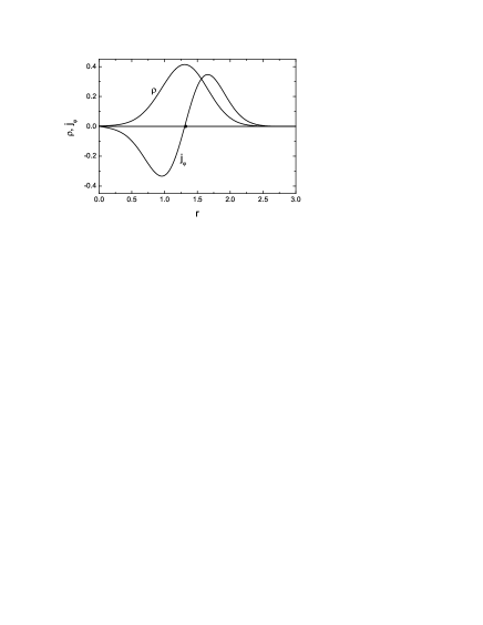
Figure 2: The radial distribution of the density ($\rho$) and azimuthal current density ($j_{\varphi}$) for three electrons in a quantum dot with $\lambda=4$ for angular momentum $M=-18$. The formation of a ring structure is apparent. Note that the currents flow in opposite directions on the inner and outer edges of the ring. The peak of $\rho$ and zero of $j_{\varphi}$ are close to the classical electron ring radius $a_{0}\approx 1.322$ marked by the dot.

Let us proceed to the examination of the current flow in quantum dots. In Fig. 2, the distributions of the charge and current density obtained from the exact diagonalizations are plotted. Since these distributions are circularly symmetric, only the radial dependences need to be shown, and moreover, the current possesses only the azimuthal component $j_{\varphi}$. Fig. 2 is obtained for a three-electron quantum dot with the interaction constant $\lambda=4$. The angular momentum is $M=-18$ and the dimensionless magnetic field is set to $B=6.78$, i. e. the midpoint of the magnetic field range where the considered state is the ground state.

We see that at these parameter values the electron ring is already well defined; the electron density at the origin drops almost to zero and peaks close to the classical value of the radius $a_{0}=(4/\sqrt{3})^{1/3}\approx 1.322$. It is interesting to observe that the currents flow in the opposite direction on the inner and the outer circumference of the ring and vanish on the classical radius.

Also, it can be noted already from Fig. 2 that the radial dependence of the current density is nearly antisymmetric with respect to the classical radius, and thus, the two currents flowing in the opposite directions nearly cancel each other. That is, there is almost no global current running along the electron ring. In order to investigate this phenomenon in more detail we numerically calculate the magnetic field dependence of the net current crossing the dot radius

$$I=\int_{0}^{\infty}j_{\varphi}(r)\,dr$$ (22)

in the ground state. The results are shown in Fig. 3. We consider angular momenta up to $|M|=20$, and use the value $\lambda=4$ for two- and three-electron dots while in the case of four electrons in the dot we set $\lambda=2$.

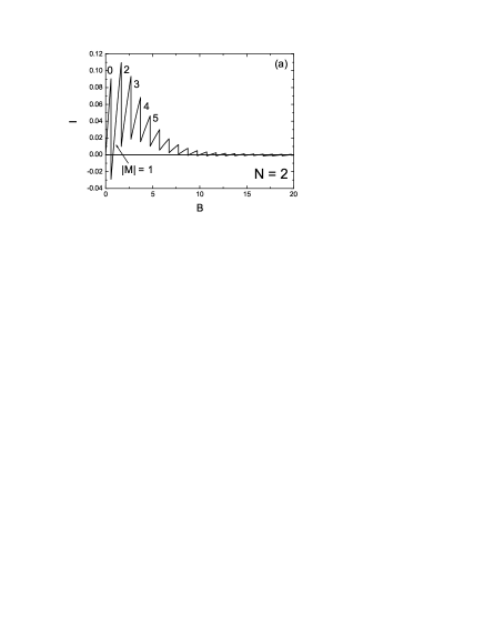
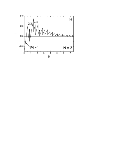
Figure 3: The net current crossing the radius of quantum dots containing two, three and four electrons calculated by exact diagonalization. The angular momenta up to $|M|=20$ are included. We observe a saw-tooth-like behavior reminiscent of persistent currents in quantum rings.

We see that these dependences display a saw-tooth-like behavior. The net current $I$ increases continuously with the magnetic field in each ground state of a given angular momentum and drops abruptly at each angular momentum transition reminding persistent currents in a ring.butt83 These currents are responsible for the dot magnetization which demonstrates a similar behavior.maksym92 Note that in two- and four-electron quantum dots where the ground state at low magnetic field has the angular momentummaarten03 $M=0$ there is no net current at zero magnetic field. In contrast, the $B=0$ ground state angular momentum in three-electron quantum dotsmikh01 is $|M|=1$ and we observe a large current at low fields.

For the sake of reference, we denote the absolute magnitude of the current jumps by $\Delta I$ and the average value of the current at the jump by $\bar{I}$. In general, both $\Delta I$ and $\bar{I}$ decrease monotonically towards zero with increasing magnetic field with a few notable exceptions occurring at very low values of the magnetic field. That is, the current oscillations tend to decrease in magnitude with increasing $B$ and the oscillatory saw-tooth pattern becomes centered around $\bar{I}=0$. The case of two electrons is rather regular and thus easy to analyse. Here, $\bar{I}$ reaches values very close to zero already at angular momenta around $|M|\approx 10$ while the behavior of three- and four-electron dots is more complicated. There are conspicuous irregularities associated with more stable states at the magic values of angular momentum, and moreover, the oscillations do not center around $\bar{I}=0$ up to higher magnetic fields. For three-electron dots $\bar{I}$ approaches zero only at highest values $|M|\approx 20$ while in four-electron dot the current oscillations do not center around zero in the considered parameter range at all.

We find that the dependence of $\bar{I}$ on the magnetic field is approximately exponential which indicates its essentially quantum-mechanical nature. Therefore, this aspect of current oscillations can not be captured by our simple quasi-classical model whose prediction is $\bar{I}\equiv 0$. But in contrast, the behavior of $\Delta I$ can be analysed and understood from a classical point of view.

For this purpose, it is sufficient to approximate the angle $\chi$ as

$$\chi\approx\frac{1}{N}\sum_{n=1}^{N}\varphi_{n},$$ (23)

and the density of the electron current along the ring can be calculated as $N$ times the average of the one-electron velocity operator. Its sole azimuthal component reads

$$j_{\varphi}(\mathbf{r})=\left(\frac{M}{r}+\frac{1}{2}BNr\right)\rho(\mathbf{r}),$$ (24)

and the total current can be estimated as

$$\begin{split}I&=\int_{0}^{\infty}dr\left(\frac{M}{r}+\frac{1}{2}BNr\right)\rho(\mathbf{r})\Big{/}\int d^{2}r\rho(\mathbf{r})\\ &\approx\left(\frac{M}{a}+\frac{1}{2}BNa\right)\int_{0}^{\infty}dr\rho(\mathbf{r})\Big{/}\int d^{2}r\rho(\mathbf{r})\\ &\approx\frac{1}{2\pi a^{2}}\left(\frac{M}{a}+\frac{1}{2}BNa\right).\end{split}$$ (25)

Thus, the current is proportional to the largest factor in the potential (16) term which was assumed to be zero when defining the approximate ring radius $a_{0}$. It means that for the calculation of the persistent current the radius of the ring has to be defined with a greater precision. So, let us equate the derivative of Eq. (16) to zero

$$\frac{d}{da}V_{0}=-\frac{1}{Na^{3}}\left(M^{2}-\frac{B^{2}N^{2}a^{4}}{4}\right)+N\left(a-\frac{N\lambda f_{N}}{2a^{2}}\right)=0.$$ (26)

Using this expression together with Eq. (17) we present the current (25) as

$$\begin{split}I&=\frac{N^{2}a}{2\pi}\left(M-\frac{1}{2}BNa^{2}\right)^{-1}\left(a-\frac{N\lambda f_{N}}{2a^{2}}\right)\\ &=-\frac{N}{2\pi B}\left\{1-\frac{\lambda f_{N}}{2}\left(\frac{NB}{2|M|}\right)^{3/2}\right\}.\end{split}$$ (27)

We observe that the magnetic field can not be compensated exactly by a discrete value of the orbital momentum. Thus, we define the critical values of the magnetic field $B_{M}$ that correspond to the exact compensation as

$$B_{M}=\frac{2|M|}{Na_{0}^{2}}=\frac{2|M|}{N}(\lambda f_{N}/2)^{-2/3}.$$ (28)

Then, introducing the magnetic field deviation $B=B_{M}+\Delta B$ we rewrite the expression for the current (27) as

$$I=-\frac{N}{2\pi B_{M}}\left\{1-\left(\frac{B_{M}+\Delta B}{B_{M}}\right)^{3/2}\right\}\approx\frac{3N\Delta B}{4\pi B_{M}^{2}}.$$ (29)

Finally, estimating the value of the current jump at the angular momentum transitions we substitute $\Delta B^{(\mathrm{max})}=2/Na_{0}^{2}$ into Eq. (29) and find

$$\Delta I=\frac{A_{N}}{\lambda^{2/3}B_{M}^{2}},\quad A_{N}=\frac{3}{2\pi(f_{N}/2)^{2/3}}.$$ (30)

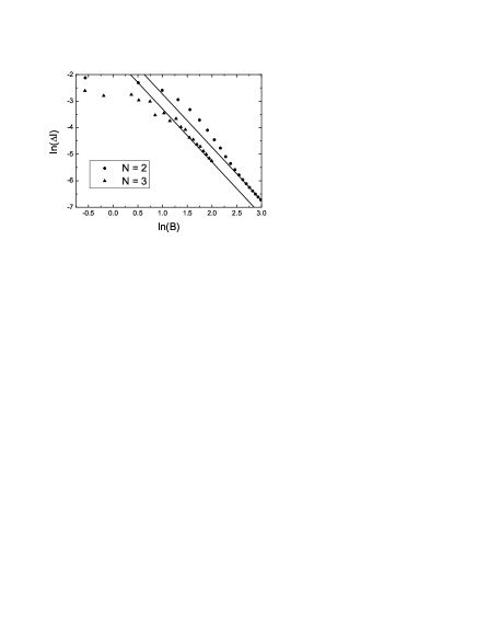
Figure 4: Double-logarithm plot of the current jumps $\Delta I$ versus the dimensionless magnetic field $B$. The symbols (full lines) denote the numerical exact diagonalization (quasi-classical) results.

Thus, our theory predicts a power-law dependence of the current jumps on the magnetic field $\Delta I\sim B^{-2}$. In order to test this prediction against the results of the numerical calculations, in Fig. 4 we plot $\Delta I$ as a function of $B$ for quantum dots containing two and three electrons. The symbols depict the numerical results from our exact diagonalizations while the straight lines describe the quasi-classical limit. One sees, that at high magnetic fields the numerical results for two- and three-electron dots indeed cross into a linear regime in a full agreement with Eq. (30).

The distribution of currents in quantum dots shown in Fig. 2 and the appearance of saw-tooth-like oscillations can be explained on the basis of the following simple considerations. The physical current consists of two components, the so-called paramagnetic current proportional to the gradient of the phase of the wave function and the contribution due to the vector-potential. The former component resembles the irrotational flow of the Euler liquid known in hydrodynamics. This current behaves as $j_{\varphi}\propto m/r$ where $m$ is the electron orbital momentum, and therefore, its vorticity (curl) is zero everywhere except at the origin. On the other hand, the vector-potential part introduces a rigid-body-like rotation with $j_{\varphi}\propto r$, and the vorticity of this component is the same at every point. As any physical system tries to minimize its energy and tends to have as small currents as possible, the two components are required to cancel each other. However, due to the very different $r$-dependences such cancelation is possible only at the classical radius of the quantum dot.

The net integrated current crossing the radius of the quantum dot is also, in general, non-zero. According to Eq. (17), an exact cancelation of the net current can be realized only for a specific value (close to the classical value) of the electron ring radius. The Coulomb repulsion between the electrons precludes the adjustment of the radius thereby causing the appearance of the uncompensated persistent current. This many-electron effect is essentially different from the single electron modelstan99 where persistent currents appear due to fixation of the electron ring radius by the confinement potential or system boundaries.

VI Local currents

In order to obtain a better understanding of the competing currents flowing in the opposite directions on the inner and outer edges of the electron ring, we will now consider the density-current correlation functions which could also be called conditional currents. In close similarity to the more familiar density-density correlators (conditional densities), these functions are obtained by pinning one of the electrons at a certain point and inspecting the distribution of currents created by the other electrons in the dot. In our calculations, we place the pinned electron at the distance equal to the classical radius $a_{0}$ from the dot center. The remaining electrons will tend to localize close to their crystallization points, distributed equidistantly along the circumference of the ring. In the quasi-classical wave function (21) the electrons are distinguishable and the motion of each of them is restricted to the vicinity of its own crystallization point. Therefore, when evaluating the quasi-classical correlation function close to these points we may dispose with the summation over the electrons and take into account only the nearest one.

When considering the correlation functions, the rotating frame coordinates $(x_{n},y_{n})$ are not the most convenient ones due to the presence of the constraint (7). Thus, having a pinned electron does not imply fixed values of its coordinates. In order to get rid of this nuisance we switch to a new set of coordinates $(\xi_{n},\eta_{n})$ which measure, respectively, the radial and angular deviations of the electrons from their crystallization positions in the laboratory frame. In the considered complex representation (4) both coordinate sets are related as

$$\exp(i[\alpha_{n}+\chi])(a+x_{n}+iy_{n})$$

$$=\exp(i\alpha_{n})(a+\xi_{n}+i\eta_{n}).$$ (31)

Separating the real and imaginary parts we are immediately led to the following two equations of the coordinate transformation

$$x_{n}+a = (\xi_{n}+a)\cos\chi+\eta_{n}\sin\chi,$$ (32a)

$$y_{n} = \eta_{n}\cos\chi-(\xi_{n}+a)\sin\chi.$$ (32b)

Performing the summation over all electrons in Eq. (32b) and fulfilling the constraint (7) we define the rotation angle $\chi$

$$\tan\chi=\frac{\sum_{n=1}^{N}\eta_{n}}{Na_{0}+\sum_{n=1}^{N}\xi_{n}}.$$ (33)

Now, inserting this expression into Eqs. (32) we solve them for ($x_{n},y_{n}$). Further inserting the solutions into Eq. (21) we obtain the quasi-classical wave function in the laboratory frame. Taking into account the fact that the quasi-classical wave function was derived in the quadratic approximation and correspondingly retaining only the necessary terms

$$\chi = \frac{\sum_{n=1}^{N}\eta_{n}}{Na_{0}}\left[1-\frac{\sum_{n=1}^{N}\xi_{n}}{Na_{0}}\right],$$ (34a)

$$x_{n} = \xi_{n},$$ (34b)

$$y_{n} = \eta_{n}-\frac{1}{N}\sum_{n=1}^{N}\eta_{n},$$ (34c)

we obtain the wave function in the laboratory frame as

$$\Psi=e^{iM\chi}e^{-B\tilde{K}/4}.$$ (35)

Here, the function $\tilde{K}$ is defined by the same expression as Eq. (21) with the variables ($x_{n},y_{n}$) replaced by the laboratory-frame coordinates ($\xi_{n},\eta_{n}$), and the angle $\chi$ is now given by Eq. (34a).

We begin by investigating the shape of the electron density lumps formed in the vicinity of their crystallization points as these results will turn out handy when discussing the currents. Straightforward integration of the $N$-particle density

$$\rho_{N}=|\Psi|^{2}=e^{-B\tilde{K}/2}$$ (36)

over the coordinates of $N-2$ electrons with the $N^{\mathrm{th}}$ electron fixed (i. e., $\xi_{N}=\eta_{N}=0$) and the first electron coordinates renamed into $\xi,\eta$, gives

$$\rho(\xi,\eta) = \int d\xi_{2}d\eta_{2}\cdots d\xi_{N-1}d\eta_{N-1}\,\rho_{N}$$ (37)

$$= \exp\left[-\frac{B}{4}\left(\frac{2N-1}{N-1}\xi^{2}+\eta^{2}\right)\right]$$

That is, the electron lump has the form of a Gaussian elongated in the azimuthal direction. The contour lines connecting the constant-density points are ellipses with the ratio of semiaxes

$$p_{N}=\sqrt{\frac{2N-1}{N-1}}=\sqrt{3},\sqrt{5/2},\sqrt{7/3}\quad\textrm{for }N=2,3,4.$$ (38)

We calculate the current-density correlation function in two steps. First, we consider the total current in the $N$-particle space and write out its component due to the first electron

$$\begin{split}&\mathbf{j}_{1,N}=\{M\nabla_{1}\chi+{\bf A}\}\rho_{N}\\ &=\Bigg{\{}\left[-\frac{M\sum_{n=1}^{N}\eta_{n}}{(Na_{0})^{2}}-\frac{B}{2}\eta_{1}\right]\mathbf{\hat{e}}_{\xi}\\ &+\left[\frac{M}{Na_{0}}-\frac{M\sum_{n=1}^{N}\xi_{n}}{(Na_{0})^{2}}+\frac{B}{2}(a_{0}+\xi_{1})\right]\mathbf{\hat{e}}_{\eta}\Bigg{\}}\rho_{N}\\ &=\mathbf{j}_{1,N}^{(p)}+\mathbf{j}_{1,N}^{(l)}.\end{split}$$ (39)

Here, the symbols $\mathbf{\hat{e}}_{\xi}$ and $\mathbf{\hat{e}}_{\eta}$ denote the unit coordinate vectors. The term independent of $\xi$ and $\eta$

$$\mathbf{j}_{1,N}^{(p)}=\left(\frac{M}{Na_{0}}+\frac{Ba_{0}}{2}\right)\mathbf{\hat{e}}_{\eta}\rho_{N}$$ (40)

leads to the persistent current which was already discussed above. Due to the integer-valued quantization of $M$ this current vanishes only at the special values of the magnetic field strength $B_{M}$ given by Eq. (28). Using Eq. (17) the term linear in $\xi$ and $\eta$ describing the local currents can be rewritten as

$$\begin{split}&\mathbf{j}_{1,N}^{(l)}=\frac{B}{2}\Bigg{\{}-\left[\eta_{1}-\frac{1}{N}\sum_{n=1}^{N}\eta_{n}\right]\mathbf{\hat{e}}_{\xi}\\ &+\left[\xi_{1}+\frac{1}{N}\sum_{n=1}^{N}\xi_{n}\right]\mathbf{\hat{e}}_{\eta}\Bigg{\}}\rho_{N}=-\frac{1}{2}[{\bf e}_{z}\times\nabla_{1}]\rho_{N},\end{split}$$ (41)

where ${\bf e}_{z}$ is the unit vector along the direction of the magnetic field. Note that this relation has the same form as that previously obtained for single-electron densities and currents.note

Now we are ready to perform the second step and calculate the correlator of the local currents by integrating the obtained expression (41) over the coordinates of $N-2$ electrons and pinning the $N^{\mathrm{th}}$ electron as it was done in obtaining Eq. (37). This procedure amounts to the replacement of the $N$-particle density $\rho_{N}$ by the density correlator (37) because the integration does not involve the coordinates of the remaining first electron. Thus, dropping the indices and denoting the first electron coordinates by ($\xi,\eta$) we arrive at the final expression for the current-density correlation function

$$\mathbf{j}(\xi,\eta)=-\frac{1}{2}[{\bf e}_{z}\times\nabla]\rho(\xi,\eta).$$ (42)

The obtained simple expression leads to important consequences. The current lines are perpendicular to the gradient of the density, and

$$\mathrm{div}\,\mathbf{j}(\xi,\eta)=-\frac{1}{2}\nabla[{\bf e}_{z}\times\nabla]\rho(\xi,\eta)=0.$$ (43)

That is, in the considered quasi-classical approximation the local currents circulating around the localized electrons are conserved. Therefore, they are physically well defined even though there is no general conservation theorem for the conditional currents (see Appendix A).

This circulatory motion of electrons is similar to the cyclotron rotation present in any single-electron model (see, e. g., Ref. lent91, ). However, due to the electron correlation and according to Eq. (42) the electrons rotate not along Larmor circles but along elliptic density contour lines. The standard quantity describing such rotational motion is the vorticity (curl) of the current field. In our case it reads

$$\begin{split}\mathrm{curl}\,\mathbf{j}(\xi,\eta)&=-\frac{1}{2}[\nabla\times[{\bf e}_{z}\times\nabla]]\rho(\xi,\eta)=-\frac{1}{2}\nabla^{2}\rho(\xi,\eta)\\ &=\frac{B}{4}\{p_{N}^{2}+1-B(p_{N}^{4}\xi^{2}+\eta^{2})\}\rho(\xi,\eta).\end{split}$$ (44)

It is worth pointing out that the vorticity is positive (i. e., it has the same sign as the vorticity of the current component due to the vector potential) at the electron crystallization points, and becomes negative at a certain distance away from them. The constant-vorticity contours are more elongated in the azimuthal direction than the density contour lines, in particular, the contour corresponding to the zero vorticity has an elliptic shape with the ratio of semiaxes equal to $p_{n}^{2}$ rather than $p_{n}$.

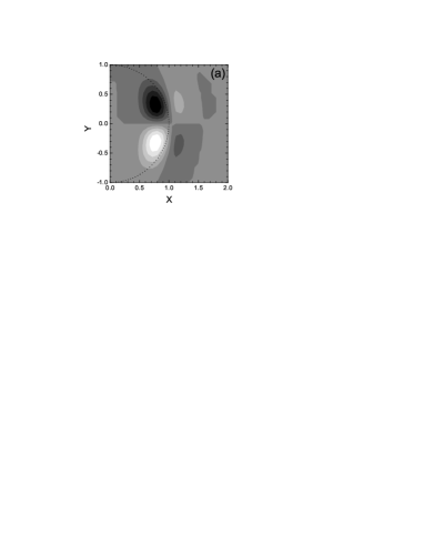
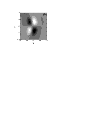
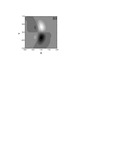
Figure 5: The divergence of the density-current correlator in a two-electron quantum dot. The angular momentum is $M=-18$. Panel (a) corresponds to the the lower end (i. e., $B=17.75$) of the magnetic field interval where this state is the ground state, panel (b) is plotted for the medium value ($B=18.25$), and panel (c) is obtained at the higher end ($B=18.75$) of this interval. Uncompensated global currents are visible. Dark (light) areas correspond to generation (extinction) of the current. The dotted curve denotes the classical radius of the quantum dot.

We illustrate the above conclusions with numerical results. The divergence of the density-current correlation function calculated for a two-electron dot is plotted in Fig. 5. We choose the value $\lambda=4$ so that the classical quantum dot radius (indicated by a dotted line in the plots) is $a_{0}=1$, and place the pinned electron at $(-1,0)$. Dark (light) areas correspond to the positive (negative) divergence, i. e. generation (extinction) of the current. The three panels of Fig. 5 show the same ground state with $|M|=18$, however, at slightly different magnetic fields. The plot in panel (a) is obtained for the lowest possible magnetic field at which this state is the ground state ($B=17.75$), panel (b) corresponds to the middle of this interval of magnetic fields ($B=18.25$), and panel (c) is obtained at the higher limit of this range ($B=18.75$). In all three plots non-conserved currents are visible. Panels (a) and (c) show a dipole-like structure corresponding to the azimuthal persistent current (40). At low magnetic fields [panel (a)] there is a net current running in the clockwise direction and at high magnetic fields we observe a net counter-clockwise current, in accordance with Eq. (40) and the saw-tooth-like behavior of Fig. 3(a). The data in panel (b) is obtained at the middle of the allowed interval of the magnetic fields. Here, $B=B_{M}$ and there is no global current. However, the divergence assumes a quadrupole-like checkerboard pattern still indicating the presence of a certain current non-conservation. This is a small higher-order effect not captured by the above quasi-classical treatment.

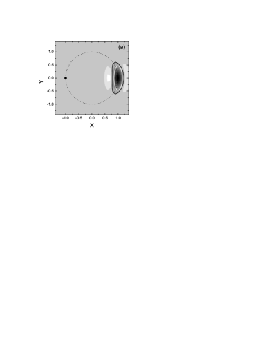
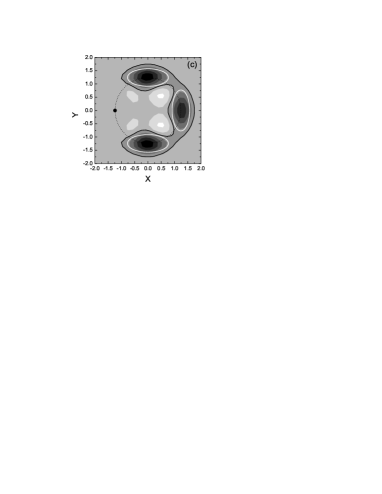
Figure 6: The curl of the density-current correlation function for quantum dots containing two, three and four electrons. The ring of the classical radius is marked by the dotted line, and one electron is pinned at the intersection of this ring with the negative part of the $x$-axis (indicated by the dot). The ground state of $M=-18$ is shown. Dark (light) areas correspond to positive (negative) vorticity, and the full black line denotes the separating zero-vorticity contour. The quasi-classical prediction for this contour is marked by the white line.

Fig. 6(a) shows the curl (vorticity) of a two-electron quantum dot. We find that the absolute values of the curl are $3$ orders of magnitude larger than the divergence, so the current non-conservation is small indeed and can be safely neglected. Here, only one plot corresponding to the middle of the allowed energy range [as in Fig. 5(b)] is shown since these plots are rather insensitive to small variations of the magnetic field. The first electron is pinned at the point $(-1,0)$ on the classical radius (the dotted line), and the second electron is crystallized in the vicinity of the opposite point $(1,0)$ and performs a cyclotron-resonance-like motion. Dark (light) areas correspond to the positive (negative) vorticity, and the full black line separates the areas corresponding to different signs of the curl. According to the theory predictions, this line is an elongated ellipsis and is marked by a white line. We see that the numerical results indicate a certain spreading and deformation of this area as the quasi-classical regime is not truly reached.

For three and four electrons we also obtain a dipole-like structure in the divergence plots since at the considered magnetic fields and angular momenta the global rotation of the electron molecule is not fully stopped, i. e. the oscillations of the current [see Figs. 3(b) and 3(c)] are not centered around zero value. In these cases, the maximum absolute values of the divergence are around $25$ times smaller than the corresponding magnitudes of the curl. The plots of the curl are shown in Figs. 6(b) and 6(c) for three and four electrons, respectively. We again consider the states with the angular momentum $M=-18$, and set the magnetic field strength to the midpoint value of the field range corresponding to the considered ground state. One electron is pinned on the negative part of the $x$-axis at the distance equal to the classical radius (marked by the dotted line) from the center. For three electrons with $\lambda=4$ this radius is $a_{0}=1.322$, and for the four-electron dot with $\lambda=2$ we have $a_{0}=1.242$. The plots in Figs. 6(b) and 6(c) again show the remaining electrons localizing close to their crystallization positions and performing the cyclotron-like motion along trajectories elongated in the azimuthal direction. The numerically calculated zero-vorticity contours are expanded and distorted with respect to the ones predicted by the quasi-classical approximation. In the case of four electrons in a dot the regions of positive vorticity even overlap.

VII Conclusion

In conclusion, we developed a quasi-classical theory based on a transformation to a rotating frame that is capable of describing the currents in quantum dots at high magnetic fields. The results show that due to the competition between the paramagnetic and vector-potential components, there arise global persistent currents running along the electron ring. At the same time, each electron may be visualized as performing individual cyclotron-like motion along elliptic trajectories elongated in the azimuthal direction. This motion is well described by the density-current correlation functions. We introduced these functions as a refinement of the suggestion to demonstrate the Wigner crystallization by calculating ordinary currents in the broken-symmetry situation, and showed that in the quasi-classical limit they are conserved, and thus, physically well defined.

Appendix A Two electrons on a 1D ring

In this section, we present a simple solvable model that, by means of a geometrical interpretation, illustrates the problems arising with the single-electron functions and correlators when discussing Wigner crystallization.

We consider two electrons moving on a 1D ring of radius $r=1$ in a perpendicular magnetic field whose behavior is described by the following Hamiltonian

$$H=-\frac{1}{2}\left\{\left(\frac{\partial}{\partial\varphi_{1}}+i\gamma\right)^{2}+\left(\frac{\partial}{\partial\varphi_{2}}+i\gamma\right)^{2}\right\}+\lambda\cos(\varphi_{1}-\varphi_{2}).$$ (45)

Here, the positions of the electrons on the ring are given by the angles $\varphi_{1,2}$, the symbol $\gamma=eBr^{2}/2c\hbar$ stands for the dimensionless vector potential, and the electron-electron interaction is modeled by the cosine function which ensures the Wigner crystallization of the electrons on the opposite ends of the diameter in the strong interaction ($\lambda\to\infty$) limit.

After the transformation

$$\Phi=\frac{1}{2}(\varphi_{1}+\varphi_{2}),\quad\varphi=\varphi_{1}-\varphi_{2}+\pi$$ (46)

the variables separate, and we rewrite the Hamiltonian (45) in the $\lambda\to\infty$ limit as

$$H=-\frac{1}{4}\left(\frac{\partial}{\partial\Phi}+2i\gamma\right)^{2}-\frac{\partial^{2}}{\partial\varphi^{2}}+\frac{\lambda}{2}\varphi^{2}.$$ (47)

whose ground-state eigenfunction is

$$\Psi(\varphi_{1},\varphi_{2})=e^{iM(\varphi_{1}+\varphi_{2})/2}\,e^{-(\varphi_{1}-\varphi_{2}+\pi)^{2}\sqrt{\lambda/8}}.$$ (48)

Here, the symbol $M$ stands for the total angular momentum. In the ground state, its value equals to the integer closest to $-2\gamma$. The corresponding many-electron density

$$\rho(\varphi_{1},\varphi_{2})=e^{-(\varphi_{1}-\varphi_{2}+\pi)^{2}\sqrt{\lambda/2}},$$ (49)

is shown in Fig. 7 by the dark stripes in the 2D many-electron space.

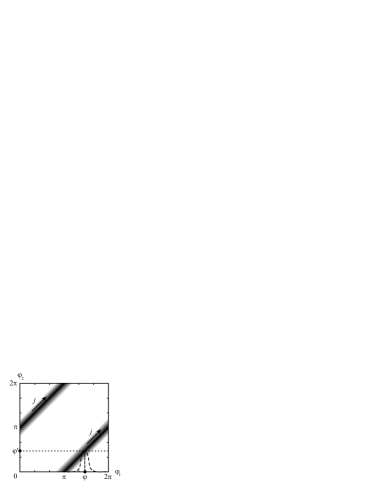
Figure 7: Many-electron density.

In this space, the current has two components related to both electrons. Its first component is given by the expectation value of the first electron velocity operator $(-i\partial/\partial\varphi_{1}+\gamma)$

$$j_{1}=(M/2+\gamma)\rho(\varphi_{1},\varphi_{2}).$$ (50)

The same result is obtained for the second component of the total current $j_{2}$. Thus, the current flows along the dark stripes as indicated by arrows in Fig. 7.

Eqs. (49), (50) and Fig. 7 contain all available information about the system. However, usually it is too difficult to consider many-electron spaces, and one resorts to simpler single-electron functions such as the density and the current obtained by integrating of Eqs. (49) and (50) over the coordinates of the second electron

$$\rho(\varphi) = \int_{0}^{2\pi}d\varphi^{\prime}\rho(\varphi,\varphi^{\prime})=\mathrm{const},$$ (51a)

$$j(\varphi) = (M/2+\gamma)\int_{0}^{2\pi}\!\!d\varphi^{\prime}\rho(\varphi,\varphi^{\prime})$$ (51b)

$$\varpropto M/2+\gamma.$$

The current expression gives the persistent current flowing along the ring. From the geometrical point of view, the above expressions are projections of the 2D many-electron density onto the abscissa axis. Naturally, they lead to a homogeneous single-electron density which provides no information about the Wigner crystal. Thus, one has to consider more sophisticated correlation functions. In our case, the density-density correlation function is given by Eq. (49) and the density-current correlation function by Eq. (50). In both cases, they are treated as functions of the first electron coordinate with the second electron coordinate fixed at the point $\varphi_{2}=\varphi^{\prime}$. Geometrically this actually means taking the cross-section of the plot shown in Fig. 7 along the dotted line $\varphi^{\prime}=\mathrm{const}$. The density-density correlation function is shown by a dashed line, and we see a lump at the point $\varphi_{1}=\varphi=\varphi^{\prime}+\pi$ which serves as a good indication of the formation of a Wigner crystal.

The current-density correlation function is not so fortunate because of the non-zero divergence

$$\frac{d}{d\varphi}j_{1}(\varphi,\varphi^{\prime})=-\sqrt{\lambda/2}(M/2+\gamma)(\varphi-\varphi^{\prime}+\pi)\rho(\varphi,\varphi^{\prime})\neq 0,$$ (52)

indicating the absence of the charge conservation. It is evident from Fig. 7 that the global current does not flow along the chosen cross-section, and the currents are escaping into other dimensions.

References

- (1) P. A. Maksym, H. Imamura, G. P. Mallon, and H. Aoki, J. Phys.: Condens. Matter 12, 299 (2000).
- (2) L. P. Kouwenhoven, D. G. Austing, and S. Tarucha, Rep. Prog. Phys. 64, 701 (2001).
- (3) S. M. Reimann and M. Manninen, Rev. Mod. Phys. 74, 1283 (2002).
- (4) L. Jacak, P. Hawrylak, and A. Wójs, Quantum Dots (Springer, Berlin, 1998).
- (5) M. B. Tavernier, E. Anisimovas, F. M. Peeters, B. Szafran, J. Adamowski, and S. Bednarek, Phys. Rev. B68, 205305 (2003).
- (6) S.-R. E. Yang and A. H. MacDonald, Phys. Rev. B66, 041304 (2002).
- (7) S. A. Mikhailov, Phys. Rev. B65, 115312 (2001).
- (8) G. Vasile, V. Gudmundsson, and A. Manolescu, in Proceedings of the 15th International Conference on High Magnetic Fields in Semiconductor Physics, (IOP, Bristol–Philadelphia, 2003), A-11 (cond-mat/0207361).
- (9) C. S. Lent, Phys. Rev. B43, 4179 (1991).
- (10) W.-C. Tan and J. C. Inkson, Phys. Rev. B60, 5626 (1999).
- (11) A. Matulis and F. M. Peeters, J. Phys.: Condens. Matter 6, 7751 (1994).
- (12) C. Yannouleas and U. Landman, Phys. Rev. B66, 115315 (2002).
- (13) C. Yannouleas and U. Landman, Phys. Rev. B68, 035326 (2003).
- (14) E. Anisimovas, A. Matulis, M. B. Tavernier, and F. M. Peeters, Phys. Rev. B69, 075305 (2004).
- (15) V. M. Bedanov and F. M. Peeters, Phys. Rev. B49, 2667 (1994).
- (16) P. A. Maksym, Phys. Rev. B53, 10871 (1996).
- (17) S. M. Reimann, M. Koskinen, and M. Manninen, Phys. Rev. Lett. 62, 8108 (2000).
- (18) S. M. Reimann, M. Koskinen, M. Manninen, and B. R. Mottelson, Phys. Rev. Lett. 83, 3270 (1999).
- (19) C. Eckardt, Phys. Rev. 47, 552 (1935).
- (20) E. Anisimovas and A. Matulis, J. Phys.: Condens. Matter 10, 601 (1998).
- (21) M. Büttiker, Y. Ymry, and R. Landauer, Phys. Lett. A 96, 365 (1983).
- (22) P. A. Maksym and T. Chakraborty, Phys. Rev. B45, 1947 (1992).
- (23) G. Vignale and P. Skudlarski, Phys. Rev. B46, 10232 (1992).